Measuring inequalities: do household surveys paint a realistic picture?
Charlotte Guénard, UMR “Développement et Sociétés”, University Paris I and IRD
Sandrine Mesplé-Somps, IRD, UMR DIAL and University Paris-Dauphine
Abstract:
The paper addresses the issue of the accuracy of standard-of-living measurements using household
survey data. First, it highlights the fact that lighter data collection processes in some developing
countries have added to consumption and income aggregate measurement errors. The paper reasserts
the need to apply reference guidelines to the measurement of household consumption in order to
compute comparable distribution indicators across countries and over time. Secondly, it contends that it
is hard to analyze inequality solely from consumption patterns without taking income and savings into
account. Two solutions are proposed for the correction of income measurement errors: by using savings
declarations and by implementing a multiple imputation procedure. The results are based on a careful
analysis of the EPM93 survey of Madagascar whose design is quite close to the LSMS household
surveys, and the ENV98 survey of Côte d'Ivoire representative of surveys conducted nowadays in most
Sub-Saharian African countries.
Keywords: household survey, inequality, missing data.
1. Introduction
In recent years, world poverty and inequality trends have prompted a great deal of research. Although it
is now recognized that around two-thirds of world inequalities come from mean living standard
divergences among countries (Schultz, 1998; Milanovic, 2002; Sala-i-Martin, 2006), the jury is still out
when it comes to world inequalities and poverty trends. There is a particular divide between Surjit S.
Bhalla and World Bank researchers1. The divergences are due mainly to the different methods used to
measure living standards and the statistical sources chosen.
In particular, it is now well known that household consumption aggregates derived from national
accounts do not generate the same level of living standards as those based on household surveys.
Taking up Ravallion (2001), Deaton (2005) shows that per capita consumption found by 277 surveys
carried out worldwide is underestimated compared with the national accounts, the ratio between the
two data sources averaging 86 percent (with a standard deviation of 31 percent). This average ratio falls
to 78 percent (standard deviation of 10 percent) for the OECD countries, although they are renowned
for having better statistical resources than other countries. Given their methods and coverage
differences2
, there is no real reason why the two information sources should provide similar
assessments of household consumption and/or income levels. In fact, it is hardly surprising to find that
they do not. What is much more worrying is that the gap widens between the two data sources (Deaton,
2005): in a sample of non-OECD countries from 1990 to 2000, the survey-based consumption growth
rate is, on average, half the rate of that based on national accounts. This observation suggests that
household surveys find it hard to capture the top end of the income distributions. This is particularly
1
See, for example, Bhalla (2002), Chen and Ravallion (2004), and Reddy and Minoiu (2007). 2
The notions of final consumption versus actual spending and of spending versus investment for housing are different in each of the two sources. In many developing countries, household consumption in the national accounts is simply a balance obtained after subtracting other forms of domestic absorption and hence cumulates the errors made upstream for the other institutional sectors. The two data sources do not agree either in terms of their population coverage: consumption in the national accounts includes the spending of "non-ordinary" households and not-for-profit institutions (workers' hostels, boarding schools, prison population, religious groups, etc.), whereas the surveys only take into account "ordinary" households’ purchases and consumption of own production. In addition, the national accountants are well aware of the problems involved in assessing the scale of illegal or informal income and subsistence income. Finally, the two sources do not necessarily use the same price deflators and may differ from year to year.
true in the case of LDCs in phases of high economic growth, such as in India, where household surveys
completely overlook the emergence of new wealthy classes (Banerjee and Piketty, 2005).3
This statistical debate – led mainly by Martin Ravallion and Angus Deaton,4 but also by national
statisticians – focuses essentially on the measurement of consumption, its mean growth and poverty,
between countries and within countries, with little mention of the problems involved in measuring
inequalities within countries. This is quite surprising since, although some people like Pyatt (2003)
warn that “[…] Household surveys are usually designed to measure average levels of income or expenditures and their design is far from optimal if the main concern is to measure the variation in
income (or expenditures) per capita across households (p. 342)”, a great deal of academic work has
been conducted in keeping with Kuznets’ work using databases on inequality computed from household surveys (Deininger and Squire, 2002; WIDER, 2005). Although the WIDER database on
inequalities now provides quality ratings, information on primary sources, definitions of aggregates and
units of analysis, in our opinion, not enough research has been done on whether household surveys can
correctly measure inequalities, especially in less developed countries (LDC). Indeed, if high inequality
levels are now deemed a brake on growth and the debate on the impact of globalization is focusing not
only on mean gaps between countries but also on within-country changes in inequality, it is crucial to
have a well-documented judgment about the household surveys’ capacity to measure inequality.
Furthermore, understanding the origins of inequalities in living standards calls for a correct
measurement of both consumption and income aggregates.
Unlike the national accounts, household surveys do not have an international protocol defining the
methods used for data collection and the calculation of living standards aggregates. However, the
World Bank’s Living Standards Measurement Study (LSMS) program set up in the 1980s proposed a
homogeneous survey design for the analysis of living standards distributions and poverty in LDCs.
3
On the other hand, national accounts systems can overestimate consumption and consumption growth by, for instance, failing to capture intermediate consumption (Deaton, 2005; Deaton and Kozel, 2005).
4
Since then, there has been a sharp rise in the number of household surveys on consumption and
income. In most Sub-Saharan African (SSA) countries, the preparation of Poverty Reduction Strategy
Papers means that National Statistics Institutes need to conduct household surveys more often than in
the past and products findings on poverty very quickly. This urgent need to produce poverty data has
prompted lighter data collection processes5. Most of them collect consumption and expenditure data in just one visit using recall questionnaires rather than consumption statements6. The number of consumption items is reduced. Local prices are not systematically compiled. This new generation of
household surveys on income and consumption is probably inferior in quality to the LSMS surveys.
This paper therefore raises the following question: are lighter current consumption and income surveys
conducted in most SSA countries able to correctly measure inequalities in standards of living?
We set out first to find out which survey biases have the greatest measurement error impact on average
living standards and inequalities. In so doing, we do not analyze the impact of random measurement
errors, as in Bound et al. (2001), Chesher and Schluter (2002), and Glewwe (2007), but measure the
scale of survey biases. There are numerous sources of potential bias that could vary in their
implications depending on the quality of the survey: (1) survey design; (2) missing values or
underestimates of certain items in the questionnaire; (3) incorrect sample design or selective
observations. Secondly, we propose a number of ways to correct them. Our conclusions are based on a
careful analysis of two surveys: the EPM93 survey of Madagascar whose design is quite close to the
LSMS household surveys; and the ENV98 survey of Côte d'Ivoire, a much simpler survey belonging to
the second generation of household surveys (see the Appendix for a detailed presentation of the
surveys).
5
Between 1980 and 1999, 69 LSMSs were conducted, 14 of which were in Sub-Saharan African (SSA) countries. Since 2000, 44 LSMSs have been carried out with only three of these in SSA countries (Ghana, Malawi and Tanzania). At the same time (between 1980 and 2009), 65 Priority Surveys have been conducted, all in SSA since 2001. A total of 29 CWIQ surveys, essentially in SSA countries (save one in Pakistan), have been done since 1997 (Source: International Household Survey Network).
6
LSMS surveys are also based on recall questionnaires, but several questions are asked to control as much as possible for recall errors and seasonal variations and interviewers visit each household at least twice.
We highlight the potentially greater uncertainty in the measurement of consumption distributions
prompted by recent changes in household survey practices in most SSA countries. We show that some
of the potential biases resulting from data collection can have a huge distributive impact, especially the
non-adjustment of price differences and sampling errors. We reassert the need to apply reference
guidelines to the measurement of household consumption in order to compute comparable
distributional indicators across countries and over time. Although we confirm that measuring
consumption is easier than measuring income aggregates, we contend that it is hard to analyze
inequality solely from consumption patterns without taking income and savings into account. We
propose two ways of correcting income measurement errors, by using savings declarations and by
implementing a multiple imputation procedure. However, in our opinion, these methods can be used to
correct income measurement errors only when the errors concerned are not too significant. This is not
the case with the new generation of household surveys in most Sub-Saharan African countries.
The remainder of the article is structured as follows. Section 2 discusses the impact of survey design
measurement errors on mean consumption aggregates and consumption inequalities depending on the
quality of the survey. Section 3 concerns the reliability of income measurement by household surveys,
with a particular focus on the correction of non-response and under-declaration biases. Section 4
analyzes biases arising from sample design and their impact on income and consumption inequality.
Section 5 concludes with some advice and recommendations on survey implementation and bias
correction.
2. New household survey practices in Sub-Saharan Africa: poorer quality data and greater uncertainty in the measurement of consumption distribution.
Methodological choices need to be clearly stated when publishing distribution indicators, otherwise it is
hard to know whether differences in observed living standards between countries reflect real gaps or
different methodologies. Yet computing options are constrained by survey designs that can prevent the
right choices being made to construct consumption aggregates. In this section, we list a number of
Household consumption aggregate definition
The guidelines developed by Deaton and Zaidi (1999) should serve as a benchmark for the definition of
consumption aggregates. Firstly, a consumption aggregate has to include: the total value of food
products consumed by the household from all possible sources (food purchases, meals purchased away
from home, own-produced food, food received from employers as payment in kind and food items
received as gifts or remittances); as well as actual rent for tenants, imputed rent for owners and housing
free of charge. Secondly, the composition of the non-food consumption sub-aggregate depends on the
approach chosen. From a welfare comparison point of view, health expenses are to be included only if
they are correctly measured and have high income elasticity; expenditure on durable goods should not
be included, but an annual rental equivalent calculated for each durable good owned by the households.
Taxes paid and loan repayments are to be excluded. Transfers and gifts to other households may be
included in the aggregate, because gifts increase the satisfaction of the person giving the gift. However,
if the consumption aggregate is calculated for a national accounts purpose, health expenses, purchases
of durable goods and housing should be included. Thirdly, relatively infrequent expenditure such as
marriages, dowries, births and funerals are liable to be included, regardless of the chosen consumption
concept, only if they have been collected for the entire household sample. Unfortunately, few
household surveys in LDCs today can apply all these recommendations. For instance, estimating the
value of services that households receive from all owned durable goods over a given time period calls
for information that is rarely collected, such as the current value of each durable good and the age and
value of the item at purchase7. Moreover, as with most second-hand data, the definition of the consumption aggregates is not given even though definition differences can have a huge influence on
standard-of-living distributions8. For example, imputing rent for households living in housing that they own has a real impact. In the Madagascan case studied here, not taking imputed rent into account
reduces the average level of consumption by 8 percent, increases the poverty rate by 9 percentage
points and raises the Gini index by over 6 percentage points, as poor people own their housing. In the
7
With no such information in the two surveys used, we are unable to evaluate the value of durable goods already owned by the household. 8
Ivoirian ENV98 survey, these effects are respectively 4 percent, 3 percentage points and 1 percentage
point.
In practice, health expenditures are often included in consumption estimates if they are everyday
expenses, but large exceptional items such as hospital operations are generally excluded. Some
estimates ignore health outlays altogether. Infrequent outlays such as marriages and funerals are
generally not included. In any case, the most important point is that methodological choices must be
clearly stated. In addition to this definition issue, other problems are raised by changing survey
practices in some LDCs, which could increase uncertainty in the measurement of consumption
distribution. These issues are listed below from the least to the most important from our point of view.
Our main results based on the EPM93 and ENV98 surveys are summarized in a single concluding
table, (Table 2, Section 5).
Level of aggregation
Since the first surveys in the LDCs, lists of consumed products have been reduced from more than
1,000 items to less than 100 items for LSMS surveys and some 50 for surveys such as the ENV98.
Shorter questionnaires save money and time. Yet the fact that this could prevent accurate estimates of
total consumption in poor LDCs has not been settled by the literature except by Deaton and Grosh
(2000), who consider that using about 70 to 100 items could be a reasonable solution even if it were to
slightly underestimate total consumption.
Recall reference period
It is well known that overly long recall periods tend to underestimate consumption because memories
fade as time goes by. Experimental work by Scott and Amenuvegbe (1990) in Ghana shows that
consumption declarations are 20 percent lower for a one week recall period than for a one day recall
period. Appleton (1996) also estimates a 25 percent gap between food, drink and tobacco expenditure
collected for a 7-day recall period and that collected for a 30-day recall period. Lastly, findings in India
reference period for all expenditure is one month for Indian surveys. When this period is reduced to
seven days for food outlays, as is generally the case in other countries, poverty rates fall from 43
percent to 24 percent in rural areas and from 33 percent to 20 percent in urban areas, reducing the
number of poor by 175 million.
This recall period effect also appears to be quite substantial in the case of the Madagascan EPM93
survey. Households have to choose the recall period to declare consumption (see Appendix). We
regress per capita consumption levels by products with the variable indicating the choice of declaration
frequency, while controlling for the seasonal nature of expenditure with the survey period variable. For
instance, the average levels of rice consumption (representing around 18% of current spending in
Madagascar) declared on the basis of a weekly recall period are 50% lower than the one-day recall
period amounts in rural areas, whereas there is no difference in urban areas. The Ivoirian ENV98
survey uses two recall periods: the last seven days and the previous month. As stated by Deaton and
Grosh (2000), this is the right way to proceed: the difference between one-week and one-month recall
period declarations is only 4% for food consumption, that is to say, a 2% gap in terms of total per
capita consumption but 1 Gini coefficient percentage point. This latter result confirms what Scott
(1992) noticed: growing up short period recalls is likely to exaggerate the cross household variance.
These memory effects appear to differ substantially depending on the survey design. Nevertheless,
more experimental work should be done on sub-samples, especially when data collection methodology
has changed between two survey waves in a given country.
Annualization of short-period consumption declarations and seasonal effects of consumption
The way data are annualized can also have an impact on the calculation of annual expenditure
aggregates. A study of Chinese data shows that annualizing monthly expenditure declarations by
multiplying them by twelve increases the poverty rate by 16 percentage points and the Gini index by 13
percentage points compared with the levels calculated on the basis of the expenditure statements for the
twelve months (Gibson, Huang and Rozelle, 2003). This way of extrapolating information probably
Consumption is clearly seasonal but seasonal effects are not taken into account when only a one-month
declaration is used to estimate consumption aggregates over one year. The extent to which the seasonal
nature of consumption is a problem depends on whether consumption data is collected over a full year
or for a shorter period. It is, of course, an issue in either case, but is more serious in the latter.
With respect to the seasonal nature of consumption, Jones and Ye (1997) identify the phenomenon in
the case of Côte d’Ivoire. Farming households producing cash crops (coffee, cocoa and cotton) surveyed between December and March, i.e. after the harvests, have significantly higher spending than
the others. Households producing staple food and with high levels of consumption of own production
post higher spending in April and May and lower spending from December to March. Whereas the
seasonal nature of expenditure appears to be more or less the same for coffee and cocoa producers
regardless of whether their per capita spending is above or below CFAF 100,000, poor cotton
producers are far more sensitive to the seasons than rich ones. Our analyses for Madagascar show that
surveying households in a harvest period (December to May) or a non-harvest period makes no
difference to the declarations, save for households in the first half of the living standards distribution
and those living in the Fianarantsoa and Toamasina regions. Furthermore, correcting declarations for
this seasonal bias has relatively little impact on the distribution of living standards. For instance, in the
case of the Ivoirian ENV98 survey, this correction increases the mean consumption aggregate by 2
percent and reduces the poverty rate by 1 point, without having any impact on the inequality indicators.
Surveys that do not last one year (or a long period), but contain information on the number of months
per year that food items are consumed, can contain a declaration bias in terms of the number of months
for each product consumed depending on whether the household is rich or poor, or even depending on
the subjective perception of its living standards. This problem is also linked to the seasonal nature of
consumption. Jones and Ye (1997) show that there is a positive correlation between the number of
months of consumption declared and the monthly level of expenditure. If this is the case and if data
exclude the frequency of product consumption (but simply multiply monthly figures by 12), a false
the poorest peoples’ spending than it really represents. Our calculations show that disregarding
consumption frequency has no impact on inequality, but increases the average level of consumption
and decreases poverty. These two phenomena are fairly minor in the ENV98 survey, but very high for
EPM93 survey consumption: a 75 percent increase in mean consumption and a 33 percent reduction in
the poverty rate. On the other hand, multiplying the amount of consumption of an item recalled over a
short period by the number of months that item was consumed (rather than 12) can underestimate the
mean. If the recall period is a week, for example, some households may not have purchased an item at
all in that week while others might have purchased a lot that week simply because of their patterns of
purchase. Multiplying the latter estimate by 12 is likely to exaggerate that household’s consumption, but this overestimate is offset by an underestimate for the household that happened not to purchase in
the previous week, but would have reported purchases if interviewed at a different time. Multiplying
by the number of months in which the item was consumed may give a more accurate estimate for the
former case, but still underestimates the latter case.
The value of consumption of own production and adjustment for cost-of-living differences
Three points are related to prices: improving the valuation of consumption of own production and
non-purchased consumption; correcting consumption for seasonal price variations and within-year inflation;
and finally, adjusting for regional cost-of-living differences.
In poor countries, around 50 percent of food consumption can be own-produced. Some survey
questionnaires ask household members to put a value to their consumption of own-produced food
and/or give unit purchase or sale prices. If for-own-consumption quantities are reported, the food
sub-aggregate can be calculated using prices from the food purchases section. However, own-produced
food is not of comparable quality to items bought in the market place. Self-valuation is likely to be a
much better approximation of the true “farm-gate” value rather than prices from the food purchases section. If declaration errors are suspected to be too great, mean or median prices by cluster or region
can be used to calculate the food sub-aggregate. At the same time, however, this choice can artificially
estimations. It increases the EPM93 survey mean consumption aggregate by 9 percent and the Gini
coefficient by 4 points (cf. Table 2, line 11 ). Note that there is sometimes no other choice because
neither quantities nor prices are reported; only a self-declaration of consumption of own-produced food
is given as in the case of the Ivoirian ENV98 survey. It is then impossible to have any idea of the
impact of self-valuation errors on consumption distributions.9
Within-year inflation needs to be controlled for if data collection lasts over a long period with inflation.
For instance, the EPM93 survey in Madagascar was conducted over a ten-month period with inflation
running at roughly 40 percent. As can be seen from table 2, when comparing lines 9 and 10, correcting
for within-year inflation reduces the mean consumption aggregate by 22 percent and increases the Gini
index by 2 percentage points.
If the aim of the consumption aggregate measurement is to compare household utility levels,
consumption aggregate needs to be adjusted for cost-of-living differences (Deaton and Zaidi, 1999).
This calls for prices indices over space. In the case of LSMS-type surveys, two price sources are
available: reported individual prices and price questionnaires often added to each cluster as part of a
community questionnaire.10 Unfortunately, the new generation of surveys (like the ENV 1998) does not collect prices systematically anymore. The only available source of information is then an ancillary
source such as government price surveys. Using this source of price index could introduce statistical
noise into the consumption distribution measurement. In Côte d’Ivoire, regional indices are far
removed from reality, given that the latest regional price index dates back to 1985. In the case of
Madagascar, however, the deflators we use are precisely those calculated by the Madagascan Institute
of Statistics when it conducted the national survey (EPM) for 1993.
9
The price issue could be problematic when estimating the value of farmers’ sales. For instance, there are three ways for doing this in the Ivoirian ENV98 survey (but only one in the Madagascan survey). The first is based on declarations of the total value of crop sales; the second on quantities sold and the declared unit price, and the third applies an average sale price to quantities sold. Nevertheless, we find that these farming income choices have no real impact either on the averages or on the levels of income inequality.
10
The choice of weights for the price indices can also have a huge effect on welfare comparisons. For instance, Appleton (2003) shows from a Ugandan survey (1993-94) that taking into account interregional food basket differences changes the poverty rates: the West becomes the poorest rather than the North, and gaps between poverty rates are some 10 to 15 percentage points.
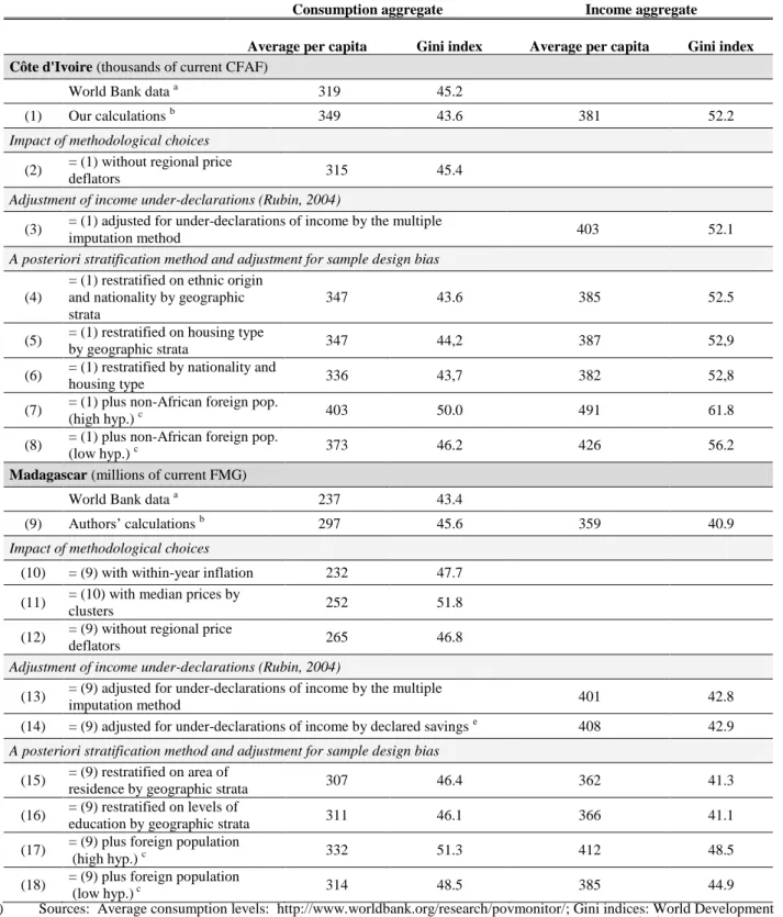
Adjustment for regional price differentials has the greatest impact on the living standards calculations
in Côte d’Ivoire (cf. concluding table, line 2 ): if regional price differences are controlled for, the average level of consumption increases by more than 10 percent in both cases (see also the comparison
of lines 9 and 12). The impact on global inequality levels comes to 2 points in the case of Côte d'Ivoire
and 0.8 in the case of Madagascar. In the case of Côte d’Ivoire, whether or not the relative price
differentials have been taken into account may explain the difference between our own inequality
calculations and those available in the World Development Indicators.
In our opinion, lighter data collection processes in most African countries may enlarge measurement
errors. Our analysis of two different survey types shows that the different methodological choices, such
as choices between two recall periods or the way of improving the valuation of consumption of own
production, have relatively little impact on distribution. However, the fact that the most recent surveys
restrict the way to consumption declarations are annualized over short periods and do not
systematically collect regional prices can give rise to considerable welfare and inequality assessment
errors.
3. Income measurement difficulties or how to deal with under-declarations and non-responses
Except in Latin American countries, living standards in LDCs are generally estimated by consumption
aggregates. This is due to the fact that income is harder to measure than consumption in poor countries.
Firstly, it is not easy to estimate private income from self-employment and micro-enterprises11 and agricultural earnings, in particular because of seasonal variations. Secondly, income declarations are
biased by non-responses and under-declarations. This section focuses on these second concerns. We
take the examples of the ENV98 and EPM93 surveys to analyse the reliability of income measurement
and investigate a number of ways to correct for non-responses and income underestimations.12
11
See de Mel et al. (2007). 12
Identifying the problem
One way of identifying income measurement error problems is to look at residual savings (balance of
income and consumption). It is well known that surveys generally find negative savings rates (Deaton,
1997). However, few papers discuss the level of and variance in these negative savings by household
living standards as we do in our analysis of the ENV98 and EPM93 surveys.
The fact that the EPM93 survey is much more detailed (see Appendix) seems to give rise to much less
biased income data than the ENV98. In the ENV98 survey, the average residual savings rate is found to
be -86 percent. It is always negative, regardless of consumption decile, and decreases with the level of
consumption. Consequently, 61 percent of households in the Ivoirian ENV98 sample have negative
residual savings, which could be normal behaviour in the event of employment loss, a bad harvest or
other negative shocks. However, over 20 percent of households consume double what their income
allows (residual savings rate lower or equal to -100 percent) and these cases are found more frequently
in the highest deciles. Moreover, we test whether there is a link between the households’ economic
difficulties and their coping strategies (using savings, selling off assets or getting into debt). However,
we find that the households with the highest rates of dissaving do face any greater economic difficulties
than other households. In the EPM93 survey, the average rate of residual savings is only - 4 percent and
average saving rates are positive and relatively high for the entire distribution with the exception of
deciles 3, 9 and 10. Only 5 percent of households in the entire sample consume double what their
current income allows.
We set out to make the income declarations consistent with the consumption declarations, even though
the latter are also subject to errors, by rectifying the income declarations using two different methods
currently available. Firstly, a correction based on declared savings data is applied to the Madagascan
EPM93 case only, because the ENV98 does not interview households about their savings flows.
Adjustment based on declared savings: a simple method
A first method implemented by Loisy (1999) in France adjusts income declarations using information
on the annual flows of savings declared by households. Income can be adjusted as follows: in the cases
where the sum of declared consumption and savings (C + S declared) is higher than the declared
income (Y declared), and the household has not taken out a consumer loan, income can be replaced by
(C + S declared); in the other cases, i.e. where income is higher than (C + S declared) and where
households have a lower income but have obtained a loan for the purchase of consumer goods, no
replacements are made. This adjustment concerns 23 percent of the Madagascan households13.
This correction raises average income by 14 percent, the average residual savings rate by 30 percentage
points and the Gini index by 2 points (see line 14 in table 2). The total savings rate for Madagascan
households is then 27 percent, a relatively high rate, as the national accounts give a rate of 2.3 percent.
The question of consistency among different sources is still present and leads us to put this result into
perspective.
This method is simple, but it requires data on annual savings flows. It can correct income declarations
affected by under-declaration biases even if these biases are correlated with income. However, it only
works if the saving declarations are not biased. If so, savings data collected by household surveys need
to be compared with other sources such as the national accounts data before this method can be used to
correct income declarations.
Accounting for missing values: possible corrections only if the bias is random
The community of survey statisticians proposes different ways of accounting for missing values14 . The
corresponding methods can be applied to income under-declarations if we consider under-declared
incomes as missing values. One relatively simple correction is to allocate the average or the median of
13
45 percent in the French “1995 Family Budget” survey (Loisy, 1999). 14
Income non-responses concern less than 1 percent of samples in the two cases studied here, but can concern a much higher percentage: in the case of the American Current Population Survey, Lillard, Smith and Welch (1986) show that the rate of non-response regarding income levels increased from 2.5 percent to 26.6 percent between 1940 and 1982, and that it was far higher for high-income professions (lawyers, doctors, etc.).
observations in the “same category”15 as the missing observation, in what is called the mean or median imputation method. This procedure is not perfect as the distribution of the new variable is incorrect
because centred values have been added; consequently, variance is underestimated. In addition, this
matching method does not allow for a large number of variables to be taken into account.
A second correction consists of estimating an explanatory model for the variable for which part of the
observations are missing, using predicted coefficients to estimate the missing values. This is called
imputation using a prediction model (see Székely and Hilgert, 1999, in their study of a range of Latin
American countries). The most sophisticated imputation method appears to be multiple imputation as
proposed by Rubin (2004). This method is based on Bayesian inference. It allows for uncertainties
about the real value of missing data by proposing different replacement values using a number of
income equation parameter selections.
However, this method, like the others, should only be used if the selection process governing the total
or partial non-response is random. In cases where the respondent is informed of the aim of the survey,
which is the case with household surveys in LDCs, there is a possibility of the selection process being
endogenous and no variable allowing selection to be ignored. One way of checking whether the
selection process is random or not is to implement the two-stage selection process proposed by
Heckmann (1979).
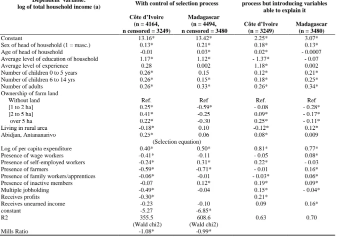
Bearing in mind this question of selection bias, we implement the multiple imputation method. The
first step is to identify households that have incorrectly declared their incomes. We select two criteria.
The first is used in the Ivoirian case: income is replaced when it is zero, because no income of any sort
is declared, and when the household’s savings rate is less than or equal to -100 percent. This first target
group represents 23 percent of the total sample. The second criterion is applied to the Madagascan
15
For example, the same characteristics in terms of age, race, gender, type of occupation, level of education and number of hours worked (Census Bureau, 2003).
case: income is recalculated when the sum of consumption and declared savings is higher than declared
income, and when the household has not contracted any debts, that is to say 23 percent of the sample.
The second step is to check for a selection bias using the Heckmann procedure (see the first two
columns in table 1). The under-declaration bias in effect appears to grow with the standard of living. As
expected, there is a positive correlation between the logarithm of per capita expenditure and the
incorrect income declaration in both samples. In the Madagascan case, the presence of independent
workers in the household is also positively correlated with the incorrect income declaration. However,
other explanatory variables are either not significant or have a negative sign. These unexpected
negative effects could suggest that individuals are consistent in that they do not tell the truth about their
income levels, multiple jobholding or their income sources by hiding the fact, for example, that they
receive unearned income. However, the data do not fully satisfy the conditions required to correctly
implement Rubin’s procedure as the selection is not ignorable16. Nonetheless, we estimate an income equation by including two groups of explanatory variables: firstly, the standard variables in a Mincer
equation (experience, education and productive assets) and, secondly, variables that capture the correct
or incorrect nature of the income value reply in order to take the selection bias into account.
In both countries, the impacts of the first group of variables are relatively standard (Table 1, last two
columns): positive and significant impact of the male head of household, the household’s number of
adults, the household’s average level of education and experience, and the head of household’s age
(these last three variables concern the Ivoirian sample only); negative impact from living in a rural area
and positive impact from living in Abidjan (but not significant from living in Antananarivo).
Households farming arable land in Madagascar have lower incomes than other households, whereas
this seems to be the case in Côte d’Ivoire only for households with less than two hectares. As regards
the second group of variables, we observe that the logarithm of per capita expenditure has a positive
significant impact. Receiving unearned income or profits increases the level of income for Madagascan
16
In this case, Rubin (Chapter 6, 2004) discusses different methods that can be used to take this bias into account, but computerized procedures with standard statistical analysis software have not yet been developed.
and Ivoirian households. In Côte d’Ivoire, the same holds true for multiple jobholders and
self-employed workers, but also for the presence of inactive members in the household. In Madagascar, the
presence of wage earners in the household, but also of inactive members, farmers and family workers
has a positive impact on the income level declared.
[Insert Table 1 here]
Lastly, we impute income on the basis of these estimations. Five imputations are made and prove
adequate17
. This income correction raises income by approximately 6 percent in Côte d’Ivoire and 13
percent in Madagascar on average (see table 2, lines 3 and 13). Whereas the Gini coefficient does not
change in Côte d’Ivoire, it increases by 2 points in Madagascar. The correction for Madagascar would appear to be convincing as it is similar to the correction made to declared savings. However, the
underestimations of income in the Ivoirian ENV98 survey do not appear to be adequately corrected. A
significant proportion of the income measurement errors is doubtless due to the fact that the ENV98
does not correctly measure informal sector and micro-enterprise earnings (see Appendix). Those
informal incomes call for specific survey methodologies, in particular to help respondents accurately
measure micro-enterprise profits. One solution for the satisfactory capture of income, especially
informal income, is to conduct informal sector surveys such as the 1-2-3 Surveys recently carried out in
a large group of African countries18.
4. Potential bias from sample designs and selective observations
Standard-of-living levels and inequality could be biased due to sample design issues. First, a sample
design based on housing automatically eliminates homeless people, who are among the most deprived
groups. Second, some households selected at the sampling stage do not actually take part in the
survey19. High-income households are likely to refrain from taking part due to the high opportunity cost of their time or to protect their private lives. Interviewers therefore have to replace them with more
17
The number of imputations depends on the difference between inter-imputation variance and intra variance. The former has to be lower than the latter. 18
See Razafindrakoto, Roubaud and Torelli (2009) 19
These non-response cases can represent up to 30 percent of the initial sample in British and American surveys (see studies quoted by Mistiaen and Ravallion, 2003).
accommodating households, which may also have lower standards of living. Lastly, some populations
may be deliberately excluded from the sample, such as non-African foreigners in the Ivoirian survey
and the entire foreign population of Madagascar.
We attempt to assess the scale of these problems in the Ivoirian and Madagascan surveys by comparing
the sample design with population censuses conducted in Côte d'Ivoire in 1998 (RGP98) and in
Madagascar in 1993 (RGP93)20. We find that some sampling biases can be substantial such as the under-representation of African foreigners in the Ivoirian case (17 percent of the total population in the
survey, compared with 26 percent in the population census), the underestimation of residents living in
permanent houses (22 percent in the survey, compared with 39 percent in the census), and the
underestimation of households living in makeshift housing – shacks and huts, especially in urban areas
– (6 percent compared with 11 percent).
However, none of the adjustments made to the sample design by the a posteriori stratification method21 has a significant impact on the income or consumption inequalities (lines 4, 5, 6, 15 and 16 in table 2).
This no doubt stems from the method itself, as it duplicates some sample values to replace the missing
values. Implicitly, it assumes that non-respondents in a given category cannot be differentiated on
average from respondents. This introduces an artificial concentration around the average values,
meaning that the variance calculations on the adjusted sample underestimate the real differences.
In both countries, part of the population living in the country has not been sampled. In Côte d'Ivoire,
32,700 individuals are deducted (source RGP98), mainly expatriate Europeans (16,028) and persons of
Lebanese origin, i.e. 0.2 percent of the country’s total population, an extremely marginal percentage in
demographic terms with no possible comparison to their economic weight. In Madagascar, the
unsampled individuals also represent the foreign population making up 0.2 percent of the total
20
In Côte d'Ivoire, the sample design for the 1998 survey was based on the 1988 General Population Census, which is problematic. In Madagascar, however, the survey was based on a census in the same year, 1993 (INSTAT, 1997).
21
The corrections consist of restratifying the survey a posteriori using an iterative cross-tabulation correction process for two criteria (nationality/geographic stratum, for instance). The households’ relative weights can then be corrected by a coefficient that restores their share in the total population before proceeding with the aggregation of incomes.
population : over a third are Europeans, 29 percent Asians, 10 percent Africans, 17 percent from the
Indian Ocean, and the remainder from the United States, the former USSR, Oceania or stateless persons
(INSTAT, 1997). Neither country covers this population in its sample design. In the case of Côte
d’Ivoire, the fact that detached houses and flats in urban areas are partly occupied by Europeans and Lebanese means that we could correct the weight of households living in this type of housing. Yet this
would be tantamount to assuming that this population has the same living standards as the African
households living in this type of housing and covered by the survey. Non-Africans tend to receive
income in line with levels in their countries of origin. We choose a different correcting process. We add
households representing these populations into the sample in keeping with the survey’s sampling rate
(13 households out of a total of 4,200 households for the ENV98 survey and 9 out of a total of 4,303
households for the EPM93 survey) and we simulate a number of living standards hypotheses (lines 7,
8, 17 and 18 in table 2). The first, “high” hypothesis assumes that this population, made up of
four-member households on average, has a monthly income of 4,500 euros per household and consumes on
average 2,290 euros per household per month (in this case, their consumption level is equivalent to that
of the ten wealthiest households).22 A second “low hypothesis” consists of allocating them a French household’s average income of approximately 2,100 euros and average consumption of around 1,100 euros.23 In Madagascar, given the make-up of the foreign population, we assume that one-third of them have living standards equivalent to Western expatriates and that the remaining two-thirds have living
standards equivalent to the country’s average. The results show the extent to which inequalities can be underestimated if non-African people are not included: whereas the average income level increases by
30 percent under the high hypothesis (11 percent under the low hypothesis) in Côte d'Ivoire and by 15
percent in Madagascar, the Gini indices increase by 9 and 8 points respectively. Under the low
hypothesis, all of these effects are halved.
22
Given that the average non-African wage in the private sector was approximately 2,600 euros in 1996 (Cogneau and Mesplé-Somps, 2002). However, expatriate salaries in the public sector are far higher than this average private wage (approximately 6,000 euros) and it can also be assumed that their spouses also receive an income.
23
This covers households that declare a positive or zero income to the tax authorities and for which the reference person is neither a student nor doing national service (source: INSEE, France).
5. Concluding remarks
As regards the controversy between national accountants and household survey supporters mentioned
in the introduction, we cannot prioritize one or other data source as long as each source, by its nature,
suffers from biases and general data quality problems. Yet these two largely independent data sources
should complement one another more. Both sources can be partially but consistently matched, as
achieved by Piketty and co-authors in the cases of India, France and the United States, by upwardly
re-evaluating high survey incomes on the basis of available tax sources (see Piketty, 2003; Banerjee and
Piketty, 2005; Piketty and Saez, 2003). In addition to tax sources, where these are available, national
accountants should use surveys to test the likelihood of national aggregates, as does the work designed
to incorporate informal sector value-added into the national accounts. The motive behind this
harmonization of data sources is not solely to allay the abovementioned controversy over the global
poverty trend given the Millennium Development Goals. This work is vital to be able to understand
intra-country sources of inequalities and can be facilitated by joint structures of accountants and
national statisticians, as is already the case in West African countries.
[Insert table 2 here]
Household survey users and designers have long been aware of all the sources of biases raised in this
paper. However, they are essentially concerned with the impact of design problems and data quality
considerations on poverty measurements rather than measurements of inequality. Moreover, given that
it is hard to correctly measure incomes, it has become standard practice to assess welfare on the basis
of current consumption rather than individual and/or household income. This choice may be justified
for poverty analyses, but we fail to see how consumption patterns alone can be used to analyze
inequalities without taking sources of income and savings into account. This consideration calls at least
for good quality data on household savings as found in the EPM93 survey and detailed income
modules.
There is no denying that more nationally representative household surveys effectively improve our
improve them and to view secondary data on inequality and poverty based on them with a critical eye.
Indeed, we have demonstrated that lighter survey designs can lead to huge errors in the calculation of
living standards, such as those due to the difficulties of controlling for regional price differentials.
Sampling designs and income under-declarations definitely have distributive impacts. Analysis of the
two surveys studied in this work shows that standards of living in each country increase and decrease in
line with the different corrections made while inequalities increase substantially. In Madagascar, the
multiple imputation method for correcting income generates a 2 point increase in the Gini index (43
compared with 41), whereas adding in the foreign population raises the Gini index by 4 to 7 points,
depending on the hypothesis chosen. In Côte d'Ivoire, the first adjustment has no impact on inequality
levels, whereas the second raises the Gini index on incomes from 52 to 56 and even 62, depending on
the scenario chosen. If nothing else, calculation methods should be clearly explained. Otherwise it is
hard to know whether deviations in living standards between two countries are due to real gaps or
methodological differences.
Are inequalities underestimated to the same extent in other countries? Does this change the country
ranking of inequalities? These questions can only be answered by extensive research, which
statisticians and other users of these databases would do well to undertake. Like Deaton, we advocate
an international cooperation initiative on survey protocol implementation and more in-depth research
into sample design errors and selective observations. Such an initiative could give rise to an accurate
Appendix: Description of the Ivoirian ENV98 and Madagascan EPM93 surveys.
The Enquête Niveau de Vie des Ménages (ENV98) was conducted by the Côte d’Ivoire National
Institute of Statistics (INS) from September 1998 to December 1998. The Enquête Permanente auprès
des Ménages (EPM93) was carried out by the National Institute of Statistics (INSTAT) from April
1993 to April 1994. The Ivoirian database contains 4,200 households (24,211 individuals) and the
Madagascan survey 4,303 households (22,710 individuals). These are relatively large samples for
LDCs. Both surveys were built to be representative at national level, with the breakdown by geographic
strata as follows: two urban strata (Abidjan and Other Towns) and three rural strata (Forest East, Forest
West and Savannah) in Côte d’Ivoire; six regions (faritany) in Madagascar (Antananarivo and
neighbouring area, Tuléar, Antsiranana, Fianarantsoa, Toamasina and Mahajanga) broken down into
urban and rural areas for each region. The Ivoirian ENV98 survey visited households once. The
EPM93 was based on repeated visits and data collection was organized differently depending on the
area: in urban areas, a cluster of 12 households was surveyed for a reference period of one month; in
rural areas, clusters of 16 households were surveyed for a reference period of seven days. The survey
was conducted in ten cycles, with each cycle corresponding to about one month of interviews in two
clusters.
Consumption data collection
The Madagascan questionnaire makes for far more detailed information on current consumption than
the Ivoirian questionnaire. For example, the Madagascan nomenclature includes 69 food items
compared with 37 for Côte d’Ivoire. In addition, there are specific modules covering annual expenditure on education and consumer durables, as well as consumption of own-produced food
expressed as a quantity of goods consumed for which the household assesses the value. For each
product, respondents choose the reference period (day, week, month or year) for the declaration of
household purchases and consumption of own production. They are then asked how often these
expenditure and consumption of own production over the last seven days and the last month and state
the number of months the product has been consumed over the year.
Income data collection
In the Ivoirian ENV98, income is quickly covered with a couple of questions on (i) how the person is
paid (fixed wage, piece-work etc.), (ii) the amount he or she is paid (estimation of the amount and unit
of time). Multiple jobholding is assessed by a single questionnaire on secondary employment
containing the same two questions. The EPM93 household questionnaire, however, goes into far more
detail about the components of income than the ENV98. For example, the EPM93 provides data on
individuals’ incomes from four potential activities in the last 12 months, the main job being the one on which the individual spends the most time (not necessarily the most lucrative), which is quite an
unusual amount of detail. As regards farming revenues, both the EPM93 and the ENV98 collect data on
farming earnings by crops. The EPM93 provides information on inputs, but not the ENV98. However,
EPM93 is less precise than the ENV98 about the valuation of farming sales: Madagascan farmers are
only asked about the value of their sales, whereas Ivoirian farmers are asked about the sale value,
quantity and unit price.
Saving data collection
Only the Madagascan EPM93 survey asked households about the flow of savings accumulated in the
current year and loans taken out. Savings in Côte d’Ivoire can only be deduced from the difference
between income and expenditure.
References
Appleton, Simon, “Regional or National Poverty Lines? The Case of Uganda in the 1990s”, Journal of
African Economies, 12 (4), 598-624, December 2003.
Bhalla, Surjit, Imagine there’s no country: Poverty, Inequality and Growth in the era of Globalization, Washington D.C., Institute for International Economics (IIE), October 2002.
Banerjee, Abhijit and Thomas Piketty, “Top Indian Incomes, 1922-2000”, The World Bank Economic
Review, 19(1), 1-20, 2005.
Bound, John, Charles Brown and Nancy Mathiowetz, “Chapter 59: Measurement Error in Survey Data”, in Heckman James J. and Edward Leamer, ed., Handbook of Econometrics, Vol. 5, 3705-3843, Amsterdam: North-Holland, 2001.
Census Bureau, “Current Population Survey Design and Methodology”, Technical Paper 63, Washington D. C., US Department of Commerce, 2003.
Chen, Shaohua and Martin Ravallion, “How the World’s Poorest have Fared Since the Early 1980s”,
The World Bank Research Observer, 19 (2), 141-170, Fall 2004.
Chesher, Andrew and Christian Schluter, “Welfare Measurement and Measurement Error”, Review of
Economic Studies, 69(2), 357-378, 2002.
Cogneau, Denis and Sandrine Mesplé-Somps, “L’économie ivoirienne, la fin du mirage ? ”, DIAL Working Paper, DT 2002/18, Paris, 2002.
Deaton, Angus, The Analysis of Household Surveys: A Microeconometric Approach to Development
Policy, Johns Hopkins University Press, World Bank, August 1997.
Deaton, Angus, “Counting the World’s Poor: Problems and Possible Solutions”, World Bank Research
Observer, 16(2), 125-147, Fall 2001.
Deaton, Angus, “Measuring Poverty in a Growing World (or Measuring Growth in a Poor World),”
Review of Economics and Statistics, 87 (1), February, 1-19, 2005.
Deaton, Angus, and Margaret Grosh “Consumption” in Margaret Grosh and paul Glewwe, ed.,
Designing Household Survey Questionnaires for Developing Countries: Lessons from Ten Years of LSMS Experience, Chapter 5, 91-133, 2000.
Deaton, Angus and Valerie Kozel, “Data and dogma: the great Indian poverty debate”, The World Bank
Research Observer, 20(2), 177-199, Fall 2005.
Deaton, Angus and Salman Zaidi, Guidelines for Constructing Consumption Aggregates for Welfare
Analysis, Princeton University and Development Research Group, World Bank: Washington DC.,
1999.
Deininger, Klaus and Lyn Squire, Revisiting Inequality: New Data Results, Global Development Network and World Bank, Washington, 2002.
De Mel, Suresh, David J. McKenzie and Christopher Woodruff, “Measuring Microenterprise Profits: Don’t Ask How the Sausage is Made”, BREAD Working Paper, 143, 2007.
Gibson, John, Jikun Huang and Scott Rozelle, “Improving Estimates of Inequality and Poverty from Urban China’s Household Income and Expenditure Survey”, Review of Income and Wealth, 49(1), 53-68, 2003.
Glewwe, Paul, “Measurement Error Bias in Estimates of Income and Income Growth among the Poor: Analytical Results and a Correction Formula”, Economic Development and Cultural Change, 56(1), 163-190, October 2007.
Heckman, James J., “Sample Selection Bias as a Specification Error”, Econometrica, 47(1), 153-161, 1979.
Jones, Christine and Xiao Ye, “Issues in Comparing Poverty Trends Over Time in Côte d’Ivoire”, World Bank Policy Research Working Paper No. 1711, January, 77 p., 1997.
INSTAT, Recensement général de la population et de l’habitat, 1993, vol. 2 Tome 1 Etat de la population; Tome 7, Ménages et habitat; Tome 2, Education, Institut National de la Statistique
Malgache, January, 1997.
Lillard, Lee, James P. Smith and Finis Welch, “What Do We Really Know about Wages ? The Importance of Non Reporting and Census Imputation”, Journal of Political Economy, 94(3), 489-506, 1986.
Loisy, Christian, “L’épargne des ménages de 1984 à 1995: disparité et diversité”, Economie et
Statistique, 324-325, 113-133, 1999.
Milanovic, Branco, “True World Income Distribution, 1988 and 1993: First Calculation Based on Household Surveys Alone,” Economic Journal, 112(476), 51-92, 2002.
Mistiaen, Johan A. and Martin Ravallion, “Survey Compliance and the Distribution of Income”, World Bank Working Paper No. 2956, January 2003.
Piketty, Thomas, “Income Inequality in France, 1901-1998”, Journal of Political Economy, Vol. 111, 1004-1042, 2003
Piketty, Thomas and Emmanuel Saez, “Income Inequality in the United States, 1913-1998”, The
Quarterly Journal of Economics, 118 (1), 1-41, February 2003
Pyatt, Graham, “Development and the Distribution of Living Standards: A Critique of the Evolving Data Base,” Review of Income and Wealth, 3(49), September, 333-358, 2003.
Ravallion, Martin, “Should Poverty Measures Be Anchored to the National Accounts?”, Special Articles, Economic and Political Weekly, 3245-3252, August 26-September 2 2000.
Ravallion, Martin, “Measuring welfare in developing countries : how well do national accounts and surveys agree?”, World Bank Policy Research Working Paper, 2665, August 2001.
Reddy, Sanjay. G. and Camelia Minoiu, “Has World Poverty Really Fallen?”, Review of Income and
Wealth, 53(3), 484-502, September 2007.
Razafindrakoto Mireille, François Roubaud and Constance Torelli, “Measuring informal sector and informal employment: the experience drawn from the 1-2-3 survey in African countries”, African
Statistical Journal, 9, November 2009.
Rubin, Donald B., Multiple Imputation for Nonresponse in Surveys. Wiley Classics Library, 287 p. (first edition 1987), 2004.
Sala-i-Martin, Xavier, “The World Distribution of Income: Falling Poverty and … Convergence Period,” Quarterly Journal of Economics, CXXI(2), 351-398, 2006.
Schultz, Paul T., “Inequality and the Distribution of Personal Income in the World: How it is Changing and Why,” Journal of Population Economics, 11(3), 307-344, 1998.
Scott, Christopher and Ben Amenuvegbe, “Effects of Recall Duration on Reporting of Household Expenditures; an Experimental Study in Ghana”, Social Dimension of Adjustment Working Paper
Series, 6, 19 p, 1990.
Scott, Christopher, “Estimation of Annual Expenditure from One-Month Cross-Sectional Data in a Household Survey,” Inter-Stat, 8, 57-65, 1992.
Székely, Miguel and Marianne Hilgert “What’s Behind The Inequality We Measure: An Investigation Using Latin American Data,” Inter-American Development Bank Working Paper, 409, December, 1999.
Visaria, Pravin, “Poverty in India during 1994-98: alternative estimates, Institute for Economic Growth,” New Delhi, processed, June 9, 2000.
WIDER, “World Income Inequality Database, V2.0a Use Guide and Data Sources,” Database on www.wider.unu.edu, 2005.
Table 1: Income equation
Dependent variable:
log of total household income (a) With control of selection process
Without taking into account selection process but introducing variables
able to explain it Côte d’Ivoire (n = 4164, n censored = 3249) Madagascar (n = 4494, n censored = 3480 Côte d’Ivoire (n = 3249) Madagascar (n = 3480) Constant 13.16* 13.42* 2.25* 3.07*
Sex of head of household (1 = masc.) 0.13* 0.21* 0.18* 0.13*
Age of head of household -0.01 0.03* 0.02* - 0.0007
Average level of education of household 1.17* 1.12* - 1.37* - 0.07
Average level of experience 0.28 0.002 1.18* 0.002
Number of children 0 to 5 years 0.26* 0.15 0.12* 0.21*
Number of children 6 to 14 yrs 0.26* 0.15* 0.18* 0.25*
Number of adults 0.26* 0.33* 0.26* 0.34*
Ownership of farm land Without land [1 to 2 ha] ]2 to 5 ha] over 5 ha Ref. 0.25* 0.41* 0.22* Ref -0.59* -0.25 -0.30 Ref. - 0.08 0.09* 0.25* Ref - 0.28* - 0.17* - 0.11*
Living in rural area -0.18* 0.10 -0.12* 0.12*
Abidjan, Antananarivo 0.25* 0.06 0.08* 0.009
(Selection equation)
Log of per capita expenditure 0.40* 0.50* 0.81* 0.77*
Presence of wage workers -0.41* -0.11 - 0.05 0.08*
Presence of self-employed workers -0.24* 0.31* 0.22* - 0.03
Presence of farmers -0.59* -0.71* - 0.01 0.16*
Presence of family workers/apprentices -0.06* -0.01 - 0.03* 0.06*
Presence of inactive members -0.07 0.12* 0.19* 0.09*
Multiple jobholding -0.49* -0.04 0.15* - 0.04*
Receives profits -0.30* 0.21*
Receives unearned income -0.23 -0.10 0.09 0.16*
constant -5.27 -6.85* R2 355.5 (Wald chi2) 608.6 (Wald chi2) 0.63 0.70 Mills Ratio -1.08* -0.99* *: variables significant at 5 %.
(a) Squared levels of age, education, experience, and number of children and adults are also introduced as explanatory variables but are not presented in this table.
Table 2: Summary of results
Consumption aggregate Income aggregate
Average per capita Gini index Average per capita Gini index
Côte d'Ivoire (thousands of current CFAF)
World Bank data a 319 45.2
(1) Our calculations b 349 43.6 381 52.2
Impact of methodological choices (2) = (1) without regional price
deflators 315 45.4
Adjustment of income under-declarations (Rubin, 2004)
(3) = (1) adjusted for under-declarations of income by the multiple
imputation method 403 52.1
A posteriori stratification method and adjustment for sample design bias (4)
= (1) restratified on ethnic origin and nationality by geographic strata
347 43.6 385 52.5
(5) = (1) restratified on housing type
by geographic strata 347 44,2 387 52,9
(6) = (1) restratified by nationality and
housing type 336 43,7 382 52,8
(7) = (1) plus non-African foreign pop.
(high hyp.) c 403 50.0 491 61.8
(8) = (1) plus non-African foreign pop.
(low hyp.) c 373 46.2 426 56.2
Madagascar (millions of current FMG)
World Bank data a 237 43.4
(9) Authors’ calculations b 297 45.6 359 40.9
Impact of methodological choices
(10) = (9) with within-year inflation 232 47.7
(11) = (10) with median prices by
clusters 252 51.8
(12) = (9) without regional price
deflators 265 46.8
Adjustment of income under-declarations (Rubin, 2004)
(13) = (9) adjusted for under-declarations of income by the multiple
imputation method 401 42.8
(14) = (9) adjusted for under-declarations of income by declared savings e 408 42.9
A posteriori stratification method and adjustment for sample design bias (15) = (9) restratified on area of
residence by geographic strata 307 46.4 362 41.3
(16) = (9) restratified on levels of
education by geographic strata 311 46.1 366 41.1
(17) = (9) plus foreign population
(high hyp.) c 332 51.3 412 48.5
(18) = (9) plus foreign population
(low hyp.) c 314 48.5 385 44.9
a) Sources: Average consumption levels: http://www.worldbank.org/research/povmonitor/; Gini indices: World Development Indicators, World Bank, 1998 and 2004; otherwise ENV98 Ivory Coast, EPM93 Madagascar, authors’ calculations.
b) Consumption aggregate includes (i) all food and food current consumer goods, consumption of own production (including non-food goods for informal entrepreneurs in the case of Madagascar); (ii) purchases of durable goods over the year; (iii) net transfers and (iv) imputed rent for house owners. Income aggregate includes (i) income from productive wage and non-wage activities over the year, from all members’ main and second jobs; (ii) income generated by household assets (dividends, rent received from rented housing and land, and imputed rent for owners); (iii) private and public net transfers. The consumption and income aggregates are calculated after eliminating data entry errors from the survey files and are deflated by regional prices.
c) Two hypotheses of non-African foreigners’ living standards:
Côte d’Ivoire: High hypothesis = available income per 4-member household of 4,500 euros per month, average consumption per household of 2,290 euros per month; Low hypothesis: available income per 4-member household of 2,100 euros per month (average French income, INSEE), average consumption per household of 1,100 euros per month.
Madagascar: one-third of foreigners have living standards equivalent to Western expatriates, and the remaining two-thirds have living standards equivalent to the country’s average.