Oscillation and waves by W. G. Harter pdf - Web Education
113
0
0
Texte intégral
(2) ©2012 W. G. Harter. Introduction. 3+ 3-. 3-. 2+ 2-. 2+ 2-. 1+ 10+. 2. Stable Hanging V=2.0. 1+ Unstable Resonance Region 10+ Stable Inverted V=2.0. Stability bands of parametric resonance of pendulums. ___________________________________________________________________________________. Sudden-cutoff-Fourier-transform of square-wave.
(3) HarterSoft –LearnIt. Unit 3 Oscillation and Resonance. 3. -- The Purest Light and a Resonance Hero – Ken Evenson (1932-2002) -- ...................................................................................5. UNIT 3. OSCILLATION AND RESONANCE!...................................................................................7 Chapter 4.1 Introduction ..................................................................................................................................................................7 Chapter 4.2 Linear oscillator response relations ............................................................................................................................8 (a) Complex phasor solutions .........................................................................................................................................................8 (b) Transient or decaying solutions ..............................................................................................................................................10 (c) Lorentz-Green stimulated response function ..........................................................................................................................11 (d) Lorentzian or Green’s function properties ..............................................................................................................................12 (e) Oscillator figures of merit: quality factors Q and q=2πQ ......................................................................................................15 (f) Beats and lifetimes ..................................................................................................................................................................16 Comparing resonant and non-resonant cases ..........................................................................................................................21 High-q resonant and non-resonant cases .................................................................................................................................21 (g) Time and frequency uncertainty relations ..............................................................................................................................23 (h) Initial conditions .....................................................................................................................................................................23 (i) Ideal Lorentz-Green functions and Smith plots .......................................................................................................................23 Exercises for Ch. 4.2: Oscillator G-functions of Forced Damped Harmonic Oscillator (FDHO) ..........................................25 Chapter 4.3 Coupled Oscillators: Eigenvalues and Eigenvectors ..............................................................................................27 (a) Equations of motion ................................................................................................................................................................28 (b) Matrix equation and reciprocity symmetry ............................................................................................................................28 (c) Rescaling and symmetrization ................................................................................................................................................29 (d) Impedance operators and general oscillation equations .........................................................................................................29 Appendix 3.A Review of Dirac Bra-ket Notation ..............................................................................................................30 (e) Change of basis and eigenstate equations ...............................................................................................................................31 Appendix 3.B Review of Change-of-Basis Transformations .............................................................................................32 Appendix 3.C Review of Eigensolutions and Diagonalization ..........................................................................................33 (f) Quadratic forms .......................................................................................................................................................................34 (g) Normal coordinates and modes ..............................................................................................................................................36 (h) Poincare periods and orbit closure ..........................................................................................................................................43 Characterizing resonances: Chaos or not? ...............................................................................................................................45 Exercises for Ch. 4.3, Ch. 4.4, and Ch. 4.8 Coupled oscillators ........................................................................................46 Chapter 4.4 Classical Oscillators and Quantum Analogs ............................................................................................................47 A classical analog of Schrodinger dynamics ......................................................................................................................47 ABCD Symmetry operator analysis and U(2) spinors ........................................................................................................48 (a) How spinors and quaternions work ........................................................................................................................................49 The “mysterious” factors of 2 ..................................................................................................................................................51 2D polarization and 3D Stokes vector S ..................................................................................................................................52 Fixed points: A port in the storm of action ..............................................................................................................................52 (b) Oscillator states by spinor rotation .........................................................................................................................................54 The A-view in {x1,x2}-basis ...................................................................................................................................................56 The C-view in {xR,xL}-basis ..................................................................................................................................................57 (c) How spinors give eigensolutions (Gone in 60 seconds!) ........................................................................................................59 (d) How spinors give time evolution ............................................................................................................................................60 B-Type Oscillation: Simple examples of balanced beats ........................................................................................................61 Exercise 4.4.1 ......................................................................................................................................................................63 Solutions to ψ-state dynamics ............................................................................................................................................64 Fig. B.3 Spin vector being rotated around B-axis during beats. The ψ-45° case is fixed on B-axis. ......................................65.
(4) ©2012 W. G. Harter. Introduction. 4. How spinors give rotation products .........................................................................................................................................66 (e) Relation of Lorentz oscillators to Schrodinger classical analog .............................................................................................66 Exercises for Ch. 4 Classical-quantum oscillator analogs ..................................................................................................67 Chapter 4.5 Coupled Oscillator Spectral Response: Green's Operators ...................................................................................69 (a) Multidimensional Green’s operators .......................................................................................................................................69 (b) Abstract Green’s operators ......................................................................................................................................................69 Example: Ion trap ....................................................................................................................................................................70 Exercises for Ch. 5 Green’s function spectral response ......................................................................................................72 Chapter 4.6 Fourier Analysis of Polychromatic Stimuli ............................................................................................................73 (a) Fourier harmonic series ..........................................................................................................................................................73 (b) Fourier integral transforms .....................................................................................................................................................77 (c) Fourier analysis in Dirac notation ...........................................................................................................................................80 (c) Fourier-Green's operator analysis ...........................................................................................................................................82 Exercises for Ch. 6 Fourier analysis ...................................................................................................................................85 Chapter 4.7 Parametric Resonance .............................................................................................................................................87 (a) Exploiting an analogy .............................................................................................................................................................89 (b) (n=2) Double-well potential and two-swing repeat ................................................................................................................90 Exercises for Ch. 7 Parametric resonance ..........................................................................................................................96 Chapter 4.8 Wave resonance in cyclic symmetry .........................................................................................................................97 (a) A 3D-oscillator with cyclic C3 symmetry ...............................................................................................................................97 (b) C3 Spectral resolution: 3rd roots of unity ..............................................................................................................................98 Modular arithmetic of mode momentum m vs. position point p .............................................................................................99 Eigenvalues and wave dispersion functions ............................................................................................................................99 (a) Shower-Curtain Models ........................................................................................................................................................101 Nth Roots of unity .................................................................................................................................................................101 (b) Solving shower curtain models by symmetry .......................................................................................................................102 (c) Wave structure and dynamics ................................................................................................................................................105 Distinguishing Ψ and Ψ*: Conjugation and time reversal ...................................................................................................105 (d) Wave superposition ...............................................................................................................................................................107 Wave phase velocity ..............................................................................................................................................................107 Group velocity and mean phase velocity ...............................................................................................................................109 Exercises for Ch. 8. ...........................................................................................................................................................111 References ......................................................................................................................................................................................111 Unit 3 Review Topics and Formulas ............................................................................................................................................113.
(5) HarterSoft –LearnIt. Unit 3 Oscillation and Resonance. 5. -- The Purest Light and a Resonance Hero – Ken Evenson (1932-2002) -. When travelers punch up their GPS coordinates they owe a debt of gratitude to an under sung hero who, alongside his colleagues and students, often toiled 18 hour days deep inside a laser laboratory lit only by the purest light in the universe.. Ken was an “Indiana Jones” of modern physics. While he may never have been called “Montana Ken,” such a name would describe a real life hero from Bozeman, Montana, whose extraordinary accomplishments in many ways surpass the fictional characters in cinematic thrillers like Raiders of the Lost Arc. Indeed, there were some exciting real life moments shared by his wife Vera, one together with Ken in a canoe literally inches from the hundred-foot drop-off of Brazil’s largest waterfall. But, such outdoor exploits, of which Ken had many, pale in the light of an in-the-lab brilliance and courage that profoundly enriched the world. Ken is one of few researchers and perhaps the only physicist to be twice listed in the Guinness Book of Records. The listings are not for jungle exploits but for his lab’s highest frequency measurement and for a speed of light determination that made c many times more precise due to his lab’s pioneering work with John Hall in laser resonance and metrology†. The meter-kilogram-second (mks) system of units underwent a redefinition largely because of these efforts. Thereafter, the speed of light c was set to 299,792,458ms-1. The meter was defined in terms of c, instead of the other way around since his time precision had so far trumped that for distance. Without such resonance precision, the Global Positioning System (GPS), the first large-scale wave space-time coordinate system, would not be possible. Ken’s courage and persistence at the Time and Frequency Division of the Boulder Laboratories in the National Bureau of Standards (now the National Institute of Standards and Technology or NIST) are legendary as are his railings against boneheaded administrators who seemed bent on thwarting his best efforts. Undaunted, Ken’s lab painstakingly exploited the resonance properties of metal-insulator diodes, and succeeded in literally counting the waves of near-infrared radiation and eventually visible light itself. Those who knew Ken miss him terribly. But, his indelible legacy resonates today as ultra-precise atomic and molecular wave and pulse quantum optics continue to advance and provide heretofore unimaginable capability. Our quality of life depends on their metrology through the Quality and Finesse of the resonant oscillators that are the heartbeats of our technology. Before being taken by Lou Gehrig’s disease, Ken began ultra-precise laser spectroscopy of unusual molecules such as HO2, the radical cousin of the more common H2O. Like Ken, such radical molecules affect us as much or more than better known ones. But also like Ken, they toil in obscurity, illuminated only by the purest light in the universe. In 2005 the Nobel Prize in physics was awarded to Glauber, Hall, and Hensch†† for laser optics and metrology. † K. M. Evenson, J.S. Wells, F.R. Peterson, B.L. Danielson, G.W. Day, R.L. Barger and J.L. Hall, Phys. Rev. Letters 29, 1346(1972). †† The Nobel Prize in Physics, 2005. http://nobelprize.org/.
(6) ©2012 W. G. Harter. Introduction. Kenneth M. Evenson – 1932-2002. 6.
(7) HarterSoft –LearnIt. 7. Unit 3 Oscillation and Resonance. Unit 3. Oscillation and Resonance Chapter 4.1 Introduction We pause our development of modern physics to consider resonance, a most important phenomenon or process. One could make the case that resonance is the single most important process in all of physics; without it we are deaf, dumb, blind, and have no telephone, radio, television or computers. Resonant amplification is needed to see or hear, and ever since the invention of the telegraph, our communication technology, power grid and electronics have all been based on it, too. Use of resonance for communication is an obvious classical application, but the introduction in Unit 2 shows that our quantum world lives and breathes resonance for its very existence. Apparently, oscillation is the currency of the universe and resonance is how nature's business is done. Without a good understanding of oscillation, resonance and waves, one should not expect to understand physics deeply if at all. Much of this book deals with relations and analogies between the older classical mechanics and the newer and more fundamental quantum theory of matter. An important part of this connection begins with a deeper understanding of resonance and resonant transfer of energy. We will introduce some key figures of merit for oscillators such as quality (Q) factors and uncertainty that also have deep significance in the development of quantum theory. We will also see how the quantum equations of motion (Schrodinger equations) are mathematically identical (analogous) to classical Hamiltonian oscillator equations, and how this helps us to appreciate both a little better. Modern applications of resonance require enormous quality factors; lately Q values of millions and billions are possible. As we will see, high quality and low uncertainty are inexorably connected. Without extremely high Q there can be no lasers, precision clocks, global positioning system (GPS), or high-speed computers. Indeed, it seems to be the case that the very quality of life for a modern civilization is strongly related to the quality Q of the oscillators in its technology. Two main types of resonance will be discussed. The first and most common classical type is the linear or additive resonance such as might occur if an oscillating electric E-field is applied to a cyclotron orbit . An example of a free linear driven oscillator equation is the following that will be treated first.. ( ). x + ω 02 x = Es cos ω st .. (4.1.1). In fact, this gives what is known as cyclotron resonance. The second type of resonance is known variously as a nonlinear or multiplicative resonance such as would occur if an oscillating magnetic B-field is applied to a cyclotron orbit. It is also called parametric resonance because the frequency parameter or spring constant k=mω2 is being stimulated. An example of a parametric resonance equation is below where its k-parameter oscillates.. (. ( )). x + A + Bcos ω st x = 0. (4.1.2). The (4.1.2) form is the one by which resonance occurs in quantum mechanics at the deepest level. However, the (4.1.1) form provides a convenient approximation for much of Nature. So, that is where we will begin..
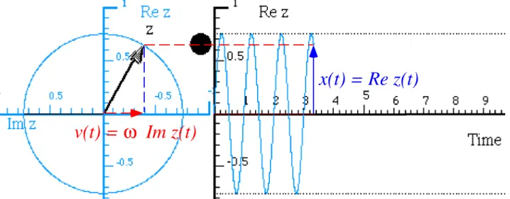
(8) ©2012 W. G. Harter. 8. Chapter 2 Linear oscillator response relations. Chapter 4.2 Linear oscillator response relations Linear forced-damped-harmonic oscillator satisfy the following classical equation of motion. d 2z dt. + 2Γ. 2. dz + ω 02 z = a dt. (4.2.1). Here a = a ( t ) is an acceleration caused by a stimulating force F ( t ) = ma ( t ) (Often F ( t ) is due to an electric field E ( t ) : F ( t ) = eE ( t ) . ) Coordinate z = z ( t ) is the response coordinate or amplitude of a particle of mass m and charge. e held by a harmonic (linear) restoring force:. ( k = ω m) , 2 0. Frestore = −kz,. (4.2.2a). We define the natural angular frequency of the oscillator in units of (radian)- Hertz = s−1 . k = 2πν 0 m. ω0 =. (4.2.2b). Also included is a "friction" term of the form of a linear damping force: Fdamping = −b. dz , dt. ( b = 2Γm). (4.2.3a). Here the decay constant is Γ=. b 2m. (4.2.3b). where b is the frictional damping coefficient. (a) Complex phasor solutions For zero stimulus (a = 0) one obtains a particular solution to (4.2.1) by letting z be a complex exponential phasor function z ( t ) = z ( 0 ) e−iω t. (4.2.4a). Euler-DeMoivre's polar-to-Cartesian expansion: reiφ = rcos φ + i rsin φ expands as follows. z ( t ) = z ( 0 ) e−iω t. = ( A + iB ) ( cos ω t − isin ω t ) , where: A = Re z ( 0 ) , and: B = Im z ( 0 ). (4.2.4b). = ( Acos ω t + Bsin ω t ) + i ( − Asin ω t + Bcos ω t ). Note: either the real or the imaginary part of the complex solution undergo undamped (Γ=0) oscillator motion introduced in Unit 1 Ch. 9. (Recall (9.8).) Two Euler forms of the initial value ( z(0) = reiα = r cos α + ir sin α ) let us conveniently derive two forms for the solution in the case of near-zero damping (Γ=0).. (. x(t) = Re z(t) = Re reiα e. (. −iω 0 t. ). = r cos α cos ω 0 t + r sin α sin ω 0 t. ). (4.2.5a). (. x(t) = Re z(t) = Re re. (. = r cos ω 0 t − α. ). iα −iω 0 t. ). (4.2.5a). Complex arithmetic gives "automatic trig-identities" and is one way it aids analysis of oscillatory phenomena. Also, as noted in Ch. 10 of Unit 1, complex phasors provide an oscillator phase space in which real and imaginary parts are proportional to position and momentum (or velocity). A sketch of a phasor diagram is shown in Fig. 4.2.1. Phasor-pairs track 2D oscillator orbits in Ch. 1 of Unit 1 and will do so in Ch. 3 of this Unit 3..
(9) HarterSoft –LearnIt. 9. Unit 3 Oscillation and Resonance. Anatomy of a Phasor z = Aeiφ = Acosφ +iAsinφ. Amplitude A=| z| = √z*z. Im z A y φ x. Phase φ = atan(y/x). 'Momentum' Im z y= Asinφ. Re z Coordinate Re z x= Acosφ. Fig. 4.2.1 Anatomy of a Phasor z=x+iy=Aeiφ = Acos φ + i Asin φ The oscillator coordinate x(t) is the real part of the phasor. x(t) = Re( Ae-i(ω t-α) ) = Acos (ω t-α). (4.2.6). Choosing a negative imaginary exponential time dependence e-iω t makes a phasor rotate clockwise. Also, it makes the imaginary part have the same sign as the instantaneous velocity or momentum since the imaginary part of e-iω t is -sin ω t with the same sign as the derivative of cos ω t. v(t) = ω Im( Ae-i(ω t-α) ) = -ω Asin (ω t-α). (4.2.7). So the phasor space is a phase-space with the momentum rescaled by ω so orbits are circles instead of ovals seen in Fig. 2.7.2. Phasors orbit clockwise just as the pendulum phase vector does in Fig. 2.7.2. Engineers, on the other hand, seem to prefer e+iω t phasors that have positive or counter clockwise rotation. Perhaps it is appropos that a physicist phasor should turn clockwise since physicists are truly the world's timekeepers. Their legacy ranges from Galileo and Huygens thru the modern ultra precise work begun by Evenson, Hall, and others at the NIST Time and Frequency division. An example of a phasor with time plot is in Fig. 4.2.2. The real and imaginary parts are each rotated by 90° so the real part matches the coordinate plot on the right-hand side of the figure. At the instant shown zcoordinate is positive and velocity is negative, corresponding to an instantaneous phase angle of φ = -30°. Modern calculators have P ↔ R buttons for converting between polar and rectangular (Cartesian) coordinates. This is aimed mainly at converting between polar form (4.2.4a) and Cartesian form (4.2.4b) or (4.2.6) and (4.2.7). We need to be cognizant of pitfalls in the inverse R → P conversion that requires an inverse tangent or arctangent. Let us recommend functions atan2(y,x) be used instead of horrible atan(y/x) functions. The former, like P ↔ R , always put the angle in the right quadrant. The latter rarely do!.
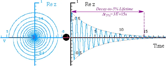
(10) ©2012 W. G. Harter. 10. Chapter 2 Linear oscillator response relations. x(t) = Re z(t) v(t) = ω Im z(t). Fig. 4.2.2 Phasor z and corresponding coordinate versus time plot for ω0=2π and Γ=0 The oscillator above is a one-Hertz ( ν 0 =1/s. or: ω 0 = 2π = 6.2832rad/s. ) oscillator. (b) Transient or decaying solutions The complex phasor e-iω·t works for damped oscillation, too. Substituting e-iω·t into (4.2.1) gives a quadratic equation for ω . The solutions are complex roots ω ± . −ω 2 − 2iΓω + ω 02 = 0, ω ± = −iΓ ± ω 02 − Γ 2. (4.28). We choose ω + the first root so phase e−iω t moves clockwise, as explained before. The resulting z(t) is called a complex transient solution, and the real part of this solution is the position x(t). ztransient ( t ) = z ( 0 ) e−Γt e. −iω Γ t. (4.2.9). It oscillates at an angular frequency ω Γ reduced slightly by .05% from ω 0 due to damping Γ =0.2. ω Γ = ω 02 − Γ 2 = ω 0 − 21 (Γ 2 / ω 0 ) + ... = 6.2831853 − 0.003183 + .. = 6.280002 + ... = 6.280001. (4.2.10). More important is exponential decay of amplitude z ( t ) by about 95% per time interval t5%=15 sec. t 5% =. 3 3 = = 15 Γ 0.2. (4.2.11a). t 4.321% =. π π = = 15.708 Γ 0.2. (4.2.11b). An easy-to-recall 5% approximation is e−3 ≅ 0.05 . A more precise one is e−π ≅ 0.04321 . A phase graph and t-plot of stimulus-free damped oscillator decay is given in Fig. 4.2.3 with ω 0 = 2π and Γ = 0.2 . This corresponds to a damped one-Hertz (or ω 0 = 2π = 6.2832rad/s. ) oscillator. A damping of Γ=0.2. reduces its natural frequency only by about 0.05% to 0.9995Hz. Fig. 4.2.3 would need a longer time, about 200 seconds, to magnify such a tiny frequency lag so it could be visible on such a graph. Also, a huge amplitude scale factor, about e20, would be needed to lift the decayed wave off the z=0 axis..
(11) HarterSoft –LearnIt. 11. Unit 3 Oscillation and Resonance. Instead of decay rates we prefer to think of lifetimes. For rough estimates we use e-3=5% lifetimes. In precise calculations, use e-π = 4.321% lifetime or. π = 15.708 seconds in (4.2.11b). Γ. Decay-to-5% Lifetime Δt 5%=3/Γ=15s. Fig. 4.2.3 Phasor z and corresponding coordinate versus time plot for ω0=2π and Γ=0.2 (c) Lorentz-Green stimulated response function The complex phasor e-iω t is particularly useful for describing resonance or stimulated oscillation. Consider a monochromatic (single frequency ωs) stimulus a (t ) = a (0) e. −iω st. .. (4.2.12). We postulate a response of the same frequency whose amplitude is proportional to the stimulus. zresponse ( t ) = Gω ω s a ( t ) (4.2.13) 0. ( ). The proportionality factor G is supposed to depend upon the stimulus frequency ωs, the natural frequency ω0 , and damping constant Γ , only. Because the equation is linear and time independent the G -factor should not depend on the amplitude As of the stimulus. It may help to think of the oscillator as a 'black box' that responds linearly to input as shown below in Fig. 4.2.4.. Lorentz-Green's Function. Response z=Gω(ωs ) as. Stimulus as(t)=Ase-iωs t. Gω(ωs )=|Gω(ωs)| e ιρ 0 0. 0. Fig. 4.2.4 Black-box diagram of oscillator response to monochromatic stimulus Now we substitute zresponse into the equation of motion (4.2.1) and solve for Gω 0 (ω s ) . The resulting Gω 0 is called a complex Lorentzian response function or classical Green’s function of the stimulus frequency ωs.. ( ). Gω ω s = 0. 1. ω 02 − ω s2 − i2Γω s. ( ). ( ). ( ). = ReGω ω s + i Im Gω ω s = Gω ω s eiρ 0 0 0. (4.2.14).
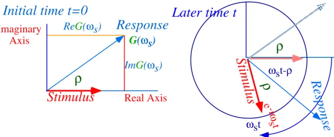
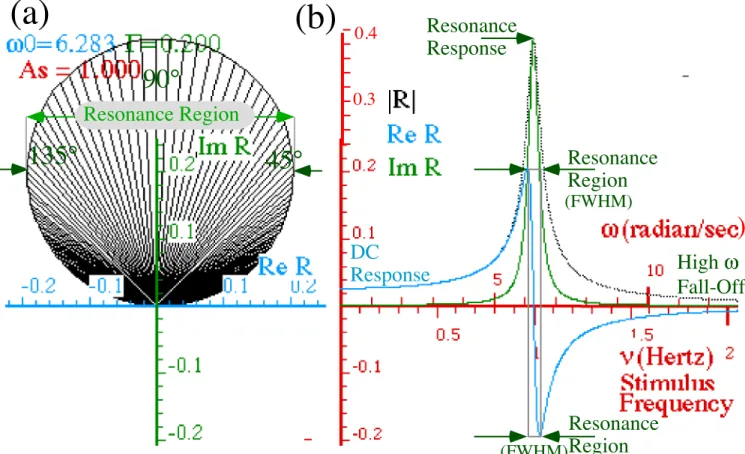
(12) ©2012 W. G. Harter. 12. Chapter 2 Linear oscillator response relations. The Lorentz-Green’s function G is a constant amplitude for fixed stimulating frequency ωs and natural ω0, so zresponse is called the steady-state stimulated response. The real and imaginary parts of the Green’s function are the two parts of the following Cartesian form of the Green’s function G. ReGω 0 (ω s ) =. (. ω 02 − ω s2. ). 2 ω 02 − ω s2. + ( 2Γω s ). 2. (4.2.15a). Im Gω 0 (ω s ) =. (ω. 2Γω s 2 0. − ω s2. ). 2. + ( 2Γω s ). 2. (4.2.15b). Then the magnitude Gω 0 (ω s ) and polar angle ρ of the polar form of G are the following: Gω 0 (ω s ) =. 1. (. ω 02 − ω s2. ). 2. + ( 2Γω s ). (4.2.15c) 2. ⎛ ( 2Γω ) ⎞ ρ = tan −1 ⎜ 2 s 2 ⎟ ⎜⎝ ω − ω ⎟⎠ 0 s. (4.2.15) The. angle ρ is the response phase lag, that is, the phase angle by which the response oscillation lags behind the phase ( −ω st ) of the stimulating oscillation. −i ω t− ρ zresponse ( t ) = Gω 0 (ω s ) a ( 0 ) e ( s ). (4.2.15). It may help to visualize stimulus and response phasors as a pair rigidly rotating at rate ωs. The response phasor lags ρ radians behind the stimulus as shown below in Fig. 4.2.5.. Initial time t=0 Imaginary Axis. ReG(ωs). Response. Later time t. G(ωs). ωst-ρ. e. ωt e-i s. ωs t. ons Resp. ρ. s. Real Axis. lu Stimu. ρ Stimulus. ImG(ωs). ρ. Fig. 4.2.5 Oscillator response and stimulus phasors rotate rigidly at angular rate ωs. The real and imaginary parts of G determine the phase lag angle ρ according to (4.2.15d). This angle is a sensitive indicator of the amount of power being delivered during resonance as discussed below. (d) Lorentzian or Greenʼs function properties Views of the Lorentz Green’s function (4.2.15) are shown in Fig. 4.2.6 for a 1 Hz oscillator with natural angular frequency ω 0 = 2π = 6.283( radian ) / s and decay constant Γ = 0.2 / s . A complex G(ωS) phasor is plotted ReGvs.ImG in Fig. 4.2.6a for a range (0<ωs <13 ) of stimulus angular frequency (or 0<νs <2 Hz of standard. frequency). In Fig. 4.2.6b the response R= G(ωS)aS due to three G-function parts ReG(ωS) (blue), ImG(ωS) (green), and | G(ωS)| (gray dots) are plotted for the same range..
(13) HarterSoft –LearnIt. 13. Unit 3 Oscillation and Resonance. (a). (b) 90°. Resonance Response. 0.3. Resonance Region. 135°. 0.4. 45°. Resonance Region (FWHM). ) DC Response. High ω Fall-Off. Resonance (FWHM)Region Fig. 4.2.6 Anatomy of oscillator Green-Lorentz response function plots The anatomy (mathematical and physical properties) of this function and related terminology are very important for the understanding resonance dynamics. They are presented here in a way that should help you remember key principles. This goes along with Exercises 4.2.3 to 4.2.5. The response magnitude |G(ωs)| is a dotted curve enveloping the others in Fig. 4.2.6b. It starts at ω s = 0 small and fairly flat ( ω s << ω 0 is called the DC response region.) and peaks near resonance point ω s = ω 0 and falls to zero for ω s >> ω 0 (high frequency fall-off). Real part ReG(ωs) dominates in the DC region. ReG(ωs) reaches a peak just shy of where it intersects the rising imaginary part ImG(ωs). ImG(ω0) achieves its peak value near resonance point ω s = ω 0 where ReG(ω0)=0 in the center of the resonance region between two Full Width at Half-Maximum (FWHM) points ω sFWHM ( ± ) = ω 0 ± Γ shown in Fig. 4.2.7. These ω sFWHM ( ± ) points are near ones that give max or min ReG(ωs), half-max ImG(ωs), and half-max |G(ωs)|. The ratio of the resonant response | G(ω0)| to the DC-response |G(0 )| is a very important number. From (4.2.15) we calculate the following (See Exercises 4.2.4 to 4.2.5.). AAF =. Gω 0 (ω 0 ) 1 / ( 2Γω 0 ) ω 0 Resonant response = = = ≡q DC response 2Γ 1 / ω 02 Gω 0 ( 0 ). (4.2.16). This ratio is about 15 in Fig. 4.2.7a and 30 in Fig. 4.2.7b. We will call this ratio the amplitude amplification factor (AAF) or angular quality (q) factor of an oscillator. A Standard Quality Factor Q=υ0/2Γ=q/2π is more commonly known1 just as standard frequency υ=ω/2π is more common than angular frequancyω=2πυ..
(14) ©2012 W. G. Harter. 14. Chapter 2 Linear oscillator response relations. (a) Γ=0.2. (b) Γ=0.1. Resonance Region FWHM =0.2. Resonance Region FWHM =0.4. 2Γ. ωFWHM(-) =ω0 − Γ ω0. ωFWHM(+) =ω0 + Γ. ωFWHM(-) =ω0 − Γ. ωFWHM(+) =ω0 + Γ. Fig. 4.2.7 Comparing Lorentz-Green resonance region for (a) Γ=0.2 and (b) Γ=0.1. Maximum and minimum points of ReG(ω) and inflection points of ImG(ω) are near region boundaries ωFWHM(±)=ω0±Γ. High values for these numbers Q, q, or AAF are good for us as humans in order that we see or hear the tiny optical or acoustical signals. The graphs for q=15 and q=30 in Fig. 4.2.7 look like impressive peaks or monuments. However, the q of a typical atom or laser resonator is much greater, in fact, millions of times higher and sharper. They are what has given modern physics its sharp teeth!.
(15) HarterSoft –LearnIt. Unit 3 Oscillation and Resonance. 15. Resonance peaks are characterized by their width as well as their height. The Full Width at HalfMaximum (FWHM) is the stimulus frequency range within which the response is at least 50% of its maximum (resonant) value of 1/ (2Γω 0 ) . At the boundaries of this range the first term (ω 02 − ω s2 )2 in the denominator of (4.2.15a-b) equals the second denominator term (2Γω s )2 .. (ω. 2 0. ). − ω s2 = 2Γω s. (For: ω s = ω sFWHM ( ± ) ). (4.2.17). If detuning difference Δ= ω s - ω 0 is much less than ω0 or ω s we may use a near-resonant approximation. ω 02 − ω s2 = (ω 0 − ω s ) (ω 0 + ω s ). (. ). (. ). ≅ ω 0 − ω s 2ω 0 ≅ ω 0 − ω s 2ω s , for: ω 0 ≈ ω s. (4.2.18). Then (4.2.17) gives FWHM boundaries at approximately the frequencies ω sFWHM ( ± ) . ω sFWHM ( ± ) = ω 0 ± Γ. (4.2.19a). ω sFWHM ( + ) − ω sFWHM ( − ) = 2Γ. (4.2.19b). The FWHM resonance region is seen to have a width of 2Γ that is 0.4 in Fig. 4.2.7a, and centered on ω0. At ω sFWHM ( ± ) response |G(ω s)| is about 50% of its maximum and its real part (4.2.15a) equals plus-or-minus its. imaginary part (4.2.15b). (See Fig. 4.2.6 or Fig. 4.2.7.). ReGω 0 (ω s ) ≅ Im Gω 0 (ω s ) , (for ω s = ω sFWHM ( ± ) ). (4.2.20). So, at the low end ω (FWHM of the resonant region, the phase lag ρ (4.2.10e) is approximately 45 ( or π /4 ) , but is −) 135 ( or 3π /4 ) at the high end ω (FWHM . ( where ReG(ω s) is plotted versus ImG(ω s) in Fig. 4.2.6a.) +) ⎧⎪ 3π / 4 ρ ω sFWHM ( ± ) ≅ ρ (ω 0 ) ± π / 4 = ⎨ ⎪⎩ π / 4. (. ). for: ω s =ω 0 +Γ for: ω s = ω 0 − Γ. (4.2.21). At exactly the resonance point (ωs=ω0) phase lag is exactly 90 ( or π / 2 ) by (4.215d). ρ (ω 0 ) = π / 2. ( for: ω s =ω 0 ). (4.2.22). The real part ReG(ω s ) of Green’s function is nearly maximum at the FWHM boundary ωsFWHM(+) and nearly minimum at ωsFWHM(-), as seen in Fig. 4.2.7. The resonant value ω s =ω 0 gives exactly zero for ReG (ω s ) and nearly a maximum for Im G (ω s ) . (See Exercises 4.2.6-7 to compute exact values.) (e) Oscillator figures of merit: quality factors Q and q=2πQ To summarize; if an oscillator of a given natural frequency ω 0 has a smaller Γ (or greater q ), then it will have greater response to a resonant ( ω s =ω 0 ) stimulus. (Recall: q = ω 0 / 2Γ is the amplification factor (4.2.12).) On the other hand, the resonant width (2Γ) in (4.2.15b) divided by ω 0 , i.e., the inverse of q , is the relative error that a stimulus frequency may have and still resonate. So, if you double an oscillator’s amplification capability, you will halve its tolerance for frequency error. Larger peak height means proportionally smaller peak width. Compare Fig. 4.2.7a with Fig. 4.2.7b..
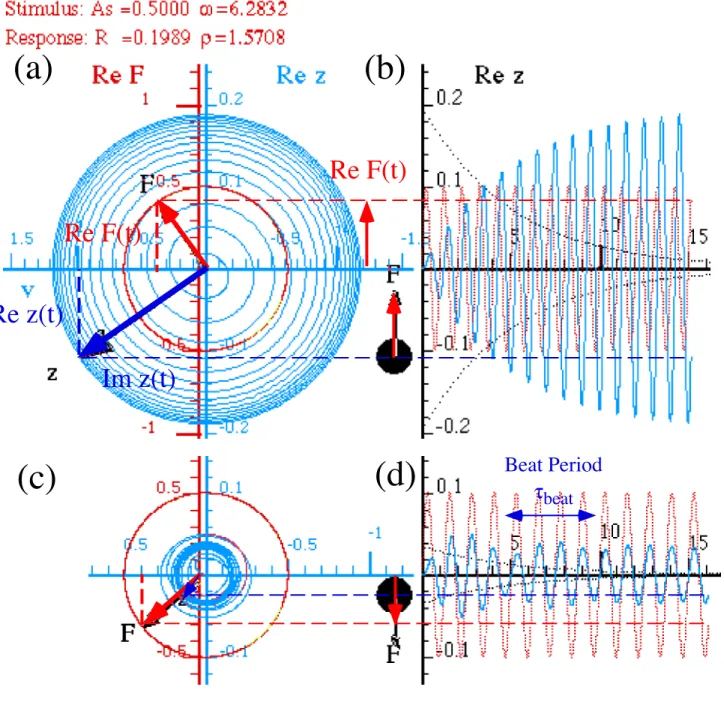
(16) ©2012 W. G. Harter. 16. Chapter 2 Linear oscillator response relations. Other important quantities are related to q . One is the number of oscillations in the 5% decay time (4.2.10). Natural oscillation frequency (4.2.9) is approximately (for Γ << ω 0 ) υ 0 = ω 0 / 2π . Multiplying by t5% gives a number n5% of oscillations in a lifetime that decaying oscillator loses 95% of its amplitude. n5% =. ω0 ω 3 ω t5% = 0 ≅ 0 = q 2π 2πΓ 2Γ. (4.2.23). For example, it takes about q = 15 oscillations to decay to 5% in Fig. 4.2.3. (Here we approximate π = 3 . Better, we use t4.321% from (4.2.11)). So, angular quality q approximates the number of “heartbeats” in the life of an oscillator. It is interesting to compare q , for your own life expectancy, to that of atoms and molecules. The most commonly used figure of oscillator merit is the standard energy quality factor Q which is defined as the ratio of an oscillator’s instantaneous energy content to energy lost each cycle. Since energy is. ( ). 2. proportional to the square of oscillator amplitude it will decay according to eΓt = e−2Γt i.e., at a rate of 2Γ times the instantaneous energy content. (See Exercise 4.2.8) dE = −2ΓE . So the relative energy lost during each cycle period (τ 0 = 1 / υ 0 ) is: ⎛ −dE ⎞ 2Γ τ0 ⎜ = ≡1 Q . ⎝ E ⎟⎠ υ 0. (4.2.24). The AAF quantity q was called the angular quality factor since 1/q is the relative loss (dE/E) per radian of phase while 1/Q is the relative loss per cycle of oscillation (f) Beats and lifetimes The quality factor q , decay constant Γ , and lifetime t5% apply as well to the birth of a resonance as they do to free oscillation decay. Suppose at t = 0 a stimulus of constant angular frequency ω s and constant amplitude a ( 0 ) is applied to a ‘cold’ oscillator ( z ( 0 ) = 0 ) . Then the sum of two solutions (4.2.8) and (4.2.15) describes the subsequent motion z(t). (Verify!) z ( t ) = ztransient ( t ) + zresponse ( t ) ≡ zdecaying ( t ) + zsteady state ( t ) = Ae−Γt e−iω Γt + Gω 0 (ω s ) a ( 0 ) e−iω st −i ω t− ρ = Ae−Γt e−iω Γt + Gω 0 (ω s ) a ( 0 ) e ( s ). (4.2.25a) (4.2.25b). The initial condition ( z ( 0 ) = 0 ) demands that the complex transient amplitude A be given by: A = − Gω 0 (ω s ) a ( 0 ) ei ρ. ( for z ( 0 ) = 0 ). (4.2.25c). so A cancels the stimulated response at t=0. Then as time progresses, the transient amplitude ztransient ( t ) dies at rate Γ and the solution eventually grows up to the steady state zresponse ( t ) , alone. An example with a resonant stimulus ( ω s = ω 0 = 2π ) is shown below in Fig. 4.2.8..
(17) HarterSoft –LearnIt. 17. Unit 3 Oscillation and Resonance. (a). (b) Re F(t) Re F(t). Re z(t) Im z(t). (c). (d). Beat Period τbeat. Fig. 4.2.8 On Resonance. (a)Response z-phasor lags ρ=90° behind stimulus F-phasor.. (ωs=ω0=2π and Γ=0.2).. (b) Time plots of Re z(t) and Re F(t). Fig. 4.2.8 Below Resonance (c)Response z-phasor lags ρ=8.05° behind stimulus F-phasor. (ωs=5.03,ω0=2π ,Γ=0.2).. (d) Time plots of Re z(t) and Re F(t). Beats are barely visible.. The length of time it takes z ( t ) to approach the steady state oscillation zresponse ( t ) is the same as the time it takes the transient part to die. So, after the 5% lifetime, the solution is mostly, i.e., 95%, steady state response. In Fig. 4.2.8b the transient dies after about t = 15sec. or about 15 oscillations. The angular quality factor q = 15 gives the number of oscillations needed for the transient to decay to less than 5% and establish 95% of a.
(18) ©2012 W. G. Harter. Chapter 2 Linear oscillator response relations. 18. resonance. The outline trace of the hidden transient is shown in Fig. 4.2.8a. It is the same as the outline of the plot in Fig. 4.2.3. Note that each response oscillation is one-quarter period to the right of its stimulating oscillation in Fig. 4.2.8b, in other words, it lags by a quarter period. This is shown more clearly by the phasor diagram in Fig. 4.2.8a where the z phasor is behind the stimulus F = a ( 0 ) e−iω st by 90° ( ρ = π / 2 ). This is consistent with (4.2.22). Since the real part of the response vanishes at resonance (ReG(ω 0 )=0), the response at ω s=ω 0 is exactly pure imaginary ( Gω 0 (ω 0 ) = Im Gω 0 (ω 0 ) ). A stimulus frequency below resonance causes transient oscillatory beat modulation. In Fig. 4.2.8c-d the angular frequency ( ω s = 5.026 ) of stimulus and steady state response is less than that of the transient ( ω Γ ≅ ω 0 = 2π = 6.28.. ). So, the transient phasor ztransient turns faster than response phasor zss-response by ω 0 − ω s = 1.25 radian/s , and it will "2π-lap" the slower phasor every 1.25/(2π) seconds. This lap rate is called the. beat frequency υbeat=ωbeat/2π . υ beat = υ s − υ 0 = ω s − ω 0 / ( 2π ) = 0.199s −1. (4.2.26). The corresponding beat period τbeat =1/νbeat is τ beat = 1 / υ s − υ 0 = 2π / ω s − ω 0 = 5.01s. (4.2.27). A beat period of about 5 sec. is seen in Fig. 4.2.8d. Beats are only visible before the transient decays below about 5%. Then the poor z(t) phasor has lost 95% of its faster transient part and can no longer "lap" the stimulus F-phasor. It is left with only the steady-state response part of (4.2.25a) and forced to "settle down" and lag dutifully at angle ρ behind the all-powerful stimulating F-phasor. In its "younger days" the transient phasor ztransient is big enough that the phasor sum z(t)= ztransient + zss-response swells up as ztransient passes the stimulus F-phasor and zss-response but then z(t) shrinks as ztransient goes on to be opposite zss-response and make a node. The interference sum z(t) experiences a beat every time ztransient laps zss response , as shown in Fig. 4.2.10 below. However, note how much smaller the transient phasor has become just in the time it takes to make a beat. It is "aging" at rate Γ while the steady-state response-phasor zss-response is just stuck ρ behind its stimulus Fphasor according to zss=G·Fstimulus. Soon z(t) falls into zss response to stay as long as Fs lasts..
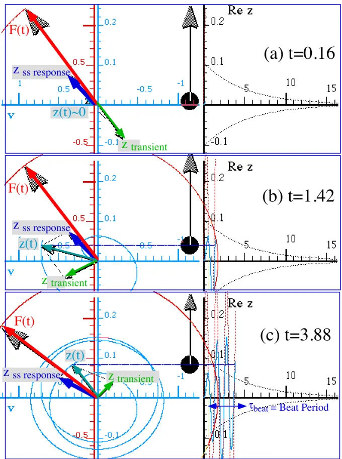
(19) HarterSoft –LearnIt. 19. Unit 3 Oscillation and Resonance. F(t). (a) t=0.16. z ss response z(t)~0 z transient F(t). (b) t=1.42. z ss response z(t) z transient F(t). (c) t=3.88 z(t). z ss response. z transient τbeat = Beat Period. Fig. 4.2.9 Beat formation. Transient phasor ztransient catches up with F-phasor and passes it..
(20) ©2012 W. G. Harter. 20. Chapter 2 Linear oscillator response relations. By counting the number of beats per second one directly measures the magnitude of the relative detuning υ s − υ0 = Δ , but not the sign of Δ. The following example in Fig. 4.2.10 has the stimulus faster than resonance by |. Δ|=0.199s−1 but with υ 0 − υ s = −0.199/s , the negative of (4.2.26).. (a). (b). Beat Period τbeat. Fig. 4.2.10 Above Resonance (a)Response z-phasor lags ρ=170.2° behind stimulus F-phasor. (ωs=7.53,ω0=2π ,Γ=0.2).. (b) Time plots of Re z(t) and Re F(t). Below is an example with half the detuning ( ω 0 − ω s = −0.63 and υ 0 − υ s = −0.1 ), and so the beats are twice as long or about 10 seconds. As ωs approaches the resonance region (ω0±Γ) the beat period gets longer still. Finally, τbeat is so long that the poor transient's beating dies below 5% before it can even make a single beat. Such is nearly the case in Fig. 4.2.8d, which looks like a half-beat that has barely come down.. Beat Period τbeat. Fig. 4.2.11 Above Resonance (a)Response z-phasor lags ρ=161.6° behind stimulus F-phasor. (ωs=6.91,ω0=2π ,Γ=0.2).. (b) Time plots of Re z(t) and Re F(t).
(21) HarterSoft –LearnIt. Unit 3 Oscillation and Resonance. 21. Comparing resonant and non-resonant cases For the below-resonance case in Fig. 4.2.8c and Fig. 4.2.9, the response phase lag according to (4.2.15d) is ρ = 0.1405 , so zss response (and eventually z(t) itself) is only 8.05° behind the stimulus. For the aboveresonance case in Fig. 4.2.10, the response zss response and z(t) lag behind by about 180° (ρ=170.2°). This a the signature of high frequency response G(∞) : it becomes nearly π out of phase with the stimulus. In contrast the low frequency or DC response G(0 ) is very nearly in phase with the stimulus. Another difference between high and low frequency response is that high frequency response goes to zero G(∞)~1/ ωS 2->0 (as ωS->∞) but low frequency resonance approaches a constant value, namely DC response = G(0 ) = 1/ ω0 2. (4.2.28) G(0 ) is just the response due to a static (DC) unit force. For high frequency oscillators, G(0 ) will be very small, but if you multiply little G(0 ) by the big angular quality factor ( q=ω0 /2Γ is the number of oscillations in the time needed to achieve 95% of a resonance), then the result 1/2ω0 Γ is exactly the resonant response amplitude G(ω0 ). (Recall (4.2.23).) In other words, the DC response (4.2.28) is the average amplitude increase which is achieved during each cycle of a unit resonant stimulus before the damping Γ really takes effect. High-q resonant and non-resonant cases For very high q quality oscillators (very low Γ) the resonant region (ω0±Γ) is so small that it may be considered non-existent. In classical Hamiltonian systems we deal with this limiting case exclusively since damping is zero by definition! Hamiltonian systems are a "transient heaven"; the beats go on forever and the transients never die or even fade away! (To a typical atom first being excited in a laser resonance with a q of fifty million, it might seem like transients live forever, too.) For infinite q there are only two values for the response phase lag angle: in-phase (ρ=0 ) and out-of-phase (ρ=π ). The out-of-phase (ρ=π ) occurs above resonance (ωs >ω0) as shown in Fig. 4.2.12a. The in-phase (ρ=0 ) case occurs below resonance (ωs <ω0) as shown in Fig. 4.2.12c. Exactly at resonance (ωs =ω0) the steady state response and the transient are both infinite and opposite so they cancel each other, and the z(t) builds up forever as shown in Fig. 4.2.12b. Each cycle of revolution adds another bit of amplitude equal to the DC response (4.2.28) just as we explained above. Fig. 4.2.12 Zero damping response ( ω0=2π ,Γ=0) (Next page) (a) Above resonance (ωs=6.91) (b) Resonance (ωs=6.28) (Stimulus amplitude reduced to show response.) (c) Below resonance (ωs=5.65).
(22) ©2012 W. G. Harter. Chapter 2 Linear oscillator response relations. (a) Above Resonance. Beat Period τbeat = 10. z(t). z transient z ss response. F(t). (b) Resonance. Beat Period τbeat = ∞. z(t). F(t). (c) Below Resonance. Beat Period τbeat = 10. z transient. z(t) F(t). z ss response. 22.
(23) HarterSoft –LearnIt. 23. Unit 3 Oscillation and Resonance. (g) Time and frequency uncertainty relations Physicists and musicians must deal with oscillators or instruments of moderate q=10-100. They may "tune" an oscillator or instrument by detecting the beats between the oscillator and a reference stimulus of much higher q. But, how accurately can a finite-q oscillator be tuned? Even if the stimulus is perfect there is a fundamental uncertainty Δω associated with the oscillator that depends on its decay rate Γ . Suppose you tune the stimulus until you no longer can detect any beats and the tuning is the best it can be. Recall that beats are transient and decay to less than 5% after time t 5% = 3 / Γ . If this time passes before half a beat it is hard to see beats as in Fig. 4.2.8d. Half a beat takes time τ half-beat = π / ω s − ω 0 . So to see a beat we need τ half-beat to be less than τ 5% or 3/Γ. π / ωs − ω0 < 3 / Γ .. This means the ω-detuning error is about equal to the decay rate Γ. (Here we approximate π~3.0, again.) ωs − ω0 > Γ. In other words, any detuning less than Γ is becoming undetectable. Total ω uncertainty is ±Γ or twice Γ that is the FWHM width Δω = 2Γ in (4.2.19). Linear frequency uncertainty is Δυ = Δω / 2π . 2Γ = Δω = 2π ·Δυ. The relative frequency uncertainty Δυ / ν 0 is therefore the inverse of the angular quality factor q. 2Γ Δω 1 Δυ = = = , ω 0 ω 0 q υ0. (4.2.29). If we think of the 5% or 3.321% lifetime of a musical note as its time uncertainty Δt , then ΔtΔυ = 3 / π ≈ 1 Δt = t 5% = 3 / Γ (4.2.30a) Δt = t 4.321% = π / Γ (4.2.30b) This is a Heisenberg relation: ΔtΔE ≈ h if energy E is Planck-related to frequency by E=hυ. (h) Initial conditions In general, the transient amplitude A = A eiα is a function of the initial conditions x ( 0 ) = x0 = Re z ( 0 ) and v0 = x ( 0 ) as well as stimulus frequency ω s and initial acceleration a ( 0 ) = a ( 0 ) . See Exercise 4.2.9. Re A = A cos α = x 0 − R cos ρ where: R = Gω (ωs ) a (0) 0. Im A = A sin α =. ν 0 − ωsR sin ρ + Γ (x 0 − R cos ρ ) ωΓ. (4.2.32). The "cold" oscillator (x0=0 =v0) of (4.2.25c) is a special case of (4.2.32). (i) Ideal Lorentz-Green functions and Smith plots When physicists speak of Lorentzian function they generally mean an ideal version of the real Lorentz response (4.2.15) with high-Q near-resonant ω s → ω 0 conditions ω 02 − ω s2 ≅ (ω 0 − ω s ) 2ω s of (4.2.18). Gω 0 (ω s ) =. ω 02. 1 1 1 1 1 1 ⎯ω⎯⎯⎯ → ≈ = L(Δ − iΓ) s →ω 0 2ω s ω 0 − ω s − iΓ 2ω 0 Δ − iΓ 2ω 0 − i2Γω s. − ω s2. (4.2.33). A complex detuning-decay δ=Δ-iΓ variable δ is defined with the real detuning Δ = ω 0 − ω s defined as before to give an ideal Lorentzian L(δ)=1/ δ below. Its imaginary part Γ / (Δ2 + Γ2 ) is what many call “a Lorentzian.” With.
(24) ©2012 W. G. Harter. 24. Chapter 2 Linear oscillator response relations. Δ=0, it becomes 1/Γ. With Γ=0, the real part becomes 1/Δ. Algebra and geometry of ideal L(δ)=1/ δ functions is. simple as given below, and 1/z-plots known as Smith plots show their geometry in Fig. 4.2.13. L(Δ − iΓ) =. 1 = Re L Δ − iΓ. + i Im L. =. iρ. =| L | e =| L | cos ρ + i | L | sin ρ =. Δ Δ + Γ2 cos ρ. Γ = | L |2 Δ + i | L |2 Γ Δ + Γ2 sin ρ 1 +i where:| L |= 2 2 2 2 2 Δ +Γ Δ +Γ Δ + Γ2. 2. +i. 2. (4.2.34). Constant Δ and Γ curves in Fig. 4.2.13 are orthogonal circles of dipolar coordinates. Recall Fig. 1.10.11. 1 cos ρ (4.2.35a) Δ Ideal Lorentz-Green’s functions Inverse decay rate 1 axis L= Δ2+ iΓ2 =|L|ei ρ |L|= 1 sin ρ Γ (Lifetime) Δ +Γ. |L| =. |L| =. 1 sin ρ Γ. (4.2.35b). Γ. ρ 1 Γ |L| 1 Δ. ρ |L|= 1 cos ρ Δ. Inverse detuning 1 axis Δ (Beat period). Fig. 4.2.13 Ideal Lorentzian in inverse rate space. (Smith life-time 1/Γ vs. beat-period 1/Δ coordinates) A circle of constant decay rate Γ and varying detuning frequency Δ has a diameter of1/Γ along the vertical of the inverse frequency space in Fig. 4.2.13. As detuning approaches zero (perfect tuning) the polar phase-lag angle angle ρ approaches π/2 and the inverse detuning or beat-period1/Δ approaches infinity. There appears to be circle of constant decay rate Γ=0.2 in Fig. 4.2.6, however, it cannot be a perfect circle, particularly in the DC region around origin. Ideal Lorentzian (4.2.34), unlike the real one, has no DC response. As decay rate Γ increases the1/Γ circle shrinks and becomes distorted by its DC “flat” at ω =0 as shown by a rather low quality (Q=1/4)-example havingΓ=2.0 and ω=2π in Fig. 4.2.14 below.. Fig. 4.2.14 Highly damped Lorentz-Green function plots with Γ=2.0 and ω=2π ..
(25) HarterSoft –LearnIt. 25. Unit 3 Oscillation and Resonance. Exercises for Ch. 4.2: Oscillator G-functions of Forced Damped Harmonic Oscillator (FDHO) Exercise 4.2.4 DC G-response of FDHO DC response Gω ( 0 ) is the amplitude caused by a unit acceleration ( a = 1) at zero stimulus frequency. This may be confusing since 0. there is no acceleration at zero frequency. A clearer definition of Gω ( 0 ) is the response due to a static force of magnitude 0. F = ma = m acting on mass m . Use this to show that the value of Gω ( 0 ) is consistent with the spring force equation (4.2.2) and 0. Hooke’s Law. Exercise 4.2.5 Resonant G-response of FDHO. (. ( ). ). Resonant response Gω ω 0 is the amplitude caused by a unit acceleration amplitude a ( t ) = 1 or force amplitude 0. (. ). ( F (t ) = m) at. ( ). resonance ω s = ω 0 . Compute the value of Gω ω 0 and show it is consistent with drag force equation (4.2.3), and that all work 0. done by F is wasted by friction. Exercise 4.2.6 The “standard” Lorentzian. In physics literature a standard Lorentzian function generally means a form L ( Δ ) = A / (Δ 2 + A2 ) with constant A. If one uses the near-resonant approximation (NRA is (4.2.18)) then L(Δ) or its derivative results from exact G-equations (4.2.15). (a) Use NRA (4.2.18) to reduce (4.2.15a-d) to a standard Lorentzian function of the detuning parameter Δ = ω s − ω 0 . (b) Show that NRA for complex response G = ReG + i Im G gives an arc of a circle in the complex plane for constant Γ and variable detuning Δ . How does this circle deviate from what appears to be a circle in Fig. 4.2.6? (Consider higher Γ values for which NRA breaks down.) Fixed Δ and varying Γ give what curve? Explain and do a ruler-and-compass construction of plots of NRA Lorentz. ( ). ( ). ( ). Green functions ReGω ω s , Im Gω ω s , and Gω ω s . 0. 0. 0. θ x=b cotθ 1 b. 1 b. x2=b2 cot2θ=b2. cos2θ sin2θ. =b2. x=b cotθ. =(1/b)sin2θ. x. x r=(1/b)sinθ. 1-sin2θ sin2θ. =. b2 sin2θ. b. y. x b θ θ. b. y=. y= r sinθ. x y. b2. =. sin θ. r. =(1/b)cosθsinθ θ r =(1/b)cosθ. θ. y. π/2−θ. θ. 1 b. b cotθ (1/b)cosθsinθ. =. b2 cosθ cosθsin2θ. =. b2 sin2θ. Exercise 4.2.7 Max and min G-values Derive equations for the extreme values for the response function or function related to G as asked below. For part (a) only use near-resonant approximation (NRA): See preceding Ex. 3.2.6.. ( ). ( ). ( ). (a) Find ω s values which give maxima for: ReGω ω s , Im Gω ω s , and Gω ω s . 0. 0. ( ). 0. (b) Do (a) for exact Gω ω s . Exact plots by calculator help check these answers. 0. (c) Find exact ω s value(s) that maximize peak KE of responding oscillator. (First show total KE=1/2 mω2 x2 for oscillation of amplitude x.).
(26) ©2012 W. G. Harter. 26. Chapter 2 Linear oscillator response relations. Exercise 4.2.8 Lifetimes Compare the number of heartbeats in your lifetime (assuming you live to a ripe old age of 100 years) to the number of oscillations in atomic and molecular lifetimes given below. (First, estimate your own angular quality factor q .) Typical atomic energy decay time is t 5% = 3 Γ = 3.4 × 10 −8 s for a green spectral 600Thz line. Compute atomic q and Q . Exercise 4.2.9 Initializing Derive the initial transient components Re A and Im A in terms of initial values x0 = x ( 0 ) , v 0 = x ( 0 ) of stimulated FDHO, response. ( ). magnitude R = G ω ω s , initial stimulus a ( 0 ) =| a | eiα , Γ, ω Γ , and ρ. 0. (Check that your total solution (4.2.25) does satisfy the initial conditions.). Exercise 4.2.10 Wiggling Old-Main lamp posts Let a static force of 10N on a lamp post cause it to bend 1cm . Upon release it vibrates at 1Hz for a minute before its amplitude dies to less than 0.05cm. Estimate ω0, Γ, and q and how much it bends 1 minute after a 1Hz oscillating force of ±1N starts. What is the bending after 2 minutes? Do this quickly by reasoning using q-factor properties and 5% mnemonics. (Points-off for too much algebra!). Exercise 4.2.11 Timing is everything! (A formula to remember) (a) Let oscillating force F(t)=Fscosωt act on a mass whose response x(t)=Gcos(ωt-ρ) also is frequency ω but with a amplitude G and a phase lag of ρ. Derive a formula for the work loop integral ∫ F dx for exactly one period of oscillation. Discuss how result relates to work done against friction in a FDHO. (Recall Ex. 3.2.5.) (b) Let oscillation x1 and x2 each have amplitude A but x1 lags x2 by phase ρ. Show by geometry that the x1 vs. x2 path is an ellipse of major axis a=A√2cos(ρ/2) and b=A√2sin(ρ/2) and area W=____. Compare this W to loop work derived in part (a).. v2 /ω. v1 /ω. x1. a. L Major axis a=A√2 cos(ρ/2) x2. L. Step 4b. Locate diagonal contact point Cb for ellipse x1 Cb. 1 Peter W. Milonni, private communication.. ρ. Asin(ρ/2). v2 /ω. Minor axis b b=A√2 sin(ρ/2). F. F. x2. ρ. L x2. F. ρ L.
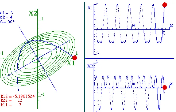
(27) HarterSoft –LearnIt. Unit 3 Oscillation and Resonance. 27. Chapter 4.3 Coupled Oscillators: Eigenvalues and Eigenvectors The Lorentz theory of preceding Ch 3.2 may be generalized to derive the spectral response of coupled oscillators. Variations of this will be used throughout the following sections. First we will consider coupled oscillator system consisting of two masses shown in Fig. 4.3.1. It is analogous to coupled pendulum pairs in Fig. 4.3.2 or to a single 2-dimensional oscillator in Fig. 4.3.3. The latter was introduced in Ch 9 of Unit 1.. k1. k12. k2. m1. .. m2. x1 = 0. x2 = 0. Fig. 4.3.1 Two 1-dimensional coupled oscillators. x2 = 0. κ. . m. . m1 θ1. m2 θ2. Fig. 4.3.2 Coupled pendulums. x1 = 0. Fig. 4.3.3 One 2-dimensional coupled oscillator.
(28) ©2012 W. G. Harter. Chapter 3 Coupled oscillation and eigensolutions. 28. (a) Equations of motion Linear (Hooke’s law) spring forces in Newton or Lagrange equations of motion for the system in Fig. 4.3.1 are 2 1 k ( ΔL ) for each spring. 2. gradients of a sum of Hooke-Law potential energies V = ∑ V=. 1 2 1 1 k x + k x2 + k x − x 2 1 1 2 2 2 2 12 1 2. V=. 1 1 k1 + k12 ) x12 − k12 x1x2 + ( k2 + k12 ) x22 ( 2 2. (. )2 (4.3.1). Kinetic energy is simply a sum of squares of velocities. 1 1 m x 2 + m x 2 2 11 2 2 2. T=. The resulting dynamic equations are the following: d ⎛ ∂T ⎞ ∂V = m1x1 = F1 = − = − k1 + k12 x1 + k12 x2 dt ⎜⎝ ∂ x1 ⎟⎠ ∂ x1. (. ). d ⎛ ∂T ⎞ ∂V = m2 x2 = F2 = − = k12 x1 − k2 + k12 x2 ⎜ ⎟ dt ⎝ ∂ x2 ⎠ ∂ x2. (. (. ). (4.3.2). Similar equations can be derived for the torsion coupled pendulum system in Fig. 4.3.2 for small angles. sin θ j ≅ θ j if θ j <<1 The torsion spring constant is κ .. ). m12θ1 = −m1gsin θ1 − κθ1 + κθ 2 ≅ −m1gθ1 − κθ1 + κθ 2 m22θ2 = κθ1 − m2 gsin θ 2 − κθ 2 ≅ κθ1 − m2 gθ 2 − κθ 2. (4.3.3). For large angles, the equation has a non-linear ‘sine-gordon’ form. The small-angle approximation yields an equation identical to (4.3.2) with x j = θ j and k1 =. g κ + = k2 l l2. k12 =. κ l2. .. (4.3.4). (b) Matrix equation and reciprocity symmetry A matrix form of the equation of motion is the following: ⎛ m1 ⎛ κ 11 κ 12 x1 ⎞ ⎜ ⎟ = −⎜ ⎜⎝ m2 ⎜⎝ κ 21 κ 22 x2 ⎟⎠. ⎞ ⎛ x1 ⎞ ⎟⎜ ⎟ ⎟⎠ ⎜⎝ x2 ⎟⎠. (4.3.5a). where we define diagonal force matrix components. κ 11 = k1 + k11, κ 22 = k2 + k22. (4.3.5b). Off-diagonal force constants are minus the original coupling constant in Fig. 4.3.1 and equation (4.3.1). k12 = −κ 12 = −κ 21 = k21 (4.3.5c) Off-diagonal symmetry of force matrices is mandatory for conservative potentials, according to Reciprocity Relations such as the following: k12 =. ∂ F1 ∂2V ∂ 2 V ∂ F2 === =k ∂ x2 ∂ x2 ∂ x1 ∂ x1 ∂ x2 ∂ x1 21. This depends on either order of partial differentiation giving the same result.. (4.3.5d).
(29) HarterSoft –LearnIt. Unit 3 Oscillation and Resonance. 29. (c) Rescaling and symmetrization Suppose we replace each coordinate ( x1, x2 ) with appropriately rescaled coordinates ( q1 = s1x1,q2 = s2 x2 ) . This can be used to symmetrize the mass factors on the q j terms. −. m1 q q q1 = κ 11 1 + κ 12 2 s1 s1 s2. −. m2 q q q2 = κ 12 1 + κ 22 2 s2 s1 s2. (4.3.6). − q1 =. κ 11 κ s q1 + 12 1 q2 ≡ Κ11q1 + Κ12 q2 m1 m1s2. − q2 =. κ 12 s2 κ q1 + 22 q2 ≡ Κ 21q1 + Κ 22 q2 m2 s1 m2. (4.3.7). The resulting mass-symmetrized equations can be made to have reciprocity symmetry, too if new constants Kij satisfy the following. The pseudo-reciprocity relations require a special scale factor ratio (4.3.8d) below. Κ 21 =. κ 12 s2 κ s −k12 = Κ12 = 12 1 = m2 s1 m1s2 m1m2. Κ11 =. κ 11 k1 + k12 = m1 m1. Κ 22 =. κ 22 k2 + k12 = m2 m2. (4.3.8a) (4.3.8b) (4.3.8c) Caution is recommended since forced symmetry may lead to unphysical results.. s2 = s1. m2 m1. (4.3.8d). (d) Impedance operators and general oscillation equations There are other coefficients besides the mass-symmetrized spring force constant matrix K ij . K ij = K ji. (4.3.9). A general linear equation may also have a resistive or frictional damping coefficient matrix Rij , and an inductive or inertial coefficient matrix Lij , as well as stimulus components fi ( t ) as in the following general equation for two coupled damped and stimulated oscillators. ⎛ L11 ⎜ ⎜⎝ L21. L12 ⎞ ⎛ q1 ⎞ ⎛ R11 ⎟⎜ ⎟ +⎜ L22 ⎟⎠ ⎜⎝ q2 ⎟⎠ ⎜⎝ R21. R12 ⎞ ⎛ q1 ⎞ ⎛ K11 K12 ⎟⎜ ⎟ +⎜ R22 ⎟⎠ ⎜⎝ q2 ⎟⎠ ⎜⎝ K 21 K 22. ⎞ ⎛ q1 ⎞ ⎛ f1 ( t ) ⎞ ⎟. ⎟⎜ ⎟ =⎜ ⎟⎠ ⎜⎝ q2 ⎟⎠ ⎜ f2 ( t ) ⎟ ⎝ ⎠. (4.3.10a). It is often the case that the reciprocity relations hold for all impedance matrices, as well as they do for potential force and acceleration components. (But don’t count on it!) Lij = L ji , Rij = R ji (4.3.10b) The equations can be written using Dirac matrix notation Zij = i Z j for each impedance matrix element, Dirac bra-ket notation q j = j q for each coordinate, and f j ( t ) = j f ( t ) for each component of the stimulus ( i, j = 1,2 ) . (See the review of Dirac bra-ket notation in Appendix 3.A below.) 2. ∑ i L j j q + i R j j q + i K j j q = i f ( t ). (4.3.10c). j=1. Removing bra i and using completeness relation ( Σ j j = 1) yields an abstract operator equations of motion. L q + R q + K q = f ( t ). + R i q + K i q = f (t) or: L i q. (4.3.10d). In electric circuits, capacitance Cij−1 is the spring matrix K ij and q = I is current flow of charge q. L i I + R i I + C −1 ∫ I dt = Vemf ( t ). (4.3.10e). , Ohm (V = R i I) , and Gauss (V = C i q = C i ∫ I dt ) . This is a combination of laws of Faraday (V = L i I).
(30) ©2012 W. G. Harter. Chapter 3 Coupled oscillation and eigensolutions. 30. Appendix 3.A Review of Dirac Bra-ket Notation. Dirac bra-ket notation is not just for quantum mechanics; it is used for all types of linear algebra. A braket a b indicates a scalar product (This is a.b in the older Gibbs notation.) ⎛ ⎜ ⎜ a b = a • b = a1 a2 an • ⎜ ⎜ ⎜ ⎝ with a row or bra vector a = a =. (. ). ⎛ b1 ⎞ ⎟ ⎜ ⎜ b2 ⎟ ⎟ = ∑ ak bk of a column or ket vector b = b = ⎜ ⎟ k ⎜ ⎜ bn ⎟⎠ ⎝. (a. 1. a2 an. b1 ⎞ ⎟ b2 ⎟ ⎟ . ⎟ bn ⎟⎠. (4.A.1). ) . Expansion of a vector in terms of a complete set of unit. vectors e1 ,e2 ,,en in Gibbs notation is . a = a1e1 + a2 e2 ++ an en . or else b = b1e1 + b2 e 2 ++ bn e n In Dirac notation we write this as. a = a1 1 + a2 2 ++ an n or else b = b1 1 + b2 2 ++ bn n . (4.A.2). Scalar product orthonormality of unit bras { 1 , 2 , n } with kets { 1 , 2 , n } is required.. ⎧⎪ 1 if j=k j k = δ jk = ⎨. ⎩⎪ 0 if j ≠ k. It implies that each bra or ket component is itself a bra-ket scalar product.. a 1 = a1, a 2 = a2 , a n = an or else, 1 b = b1, 2 b = b2 , n b = bn .. (4.A.3). (4.A.4). This in turn implies what is called completeness of the unit bases { 1 , 2 , n } and { 1 , 2 , n } . a = a 1 1 + a 2 2 ++ a n n. or else, b = 1 1 b + 2 2 b ++ n n b . The scalar product (4.A.1) is the following in full Dirac notation.. a b = a 1 1 b + a 2 2 b ++ a n n b = ∑ a k k b . If { 1 , 2 , n. }. (4.A.5). (4.A.6). is another set of n-base vectors that is orthonormal then it must be complete, too.. ⎧⎪ 1 if m=n m n = δ mn = ⎨ ⎪⎩ 0 if m ≠ n. implies: j k = j 1 1 k + j 2 2 k ++ j n n k . (4.A.7). The n-by-n matrix of scalar products between these two bases are called transformation matrices. ⎛ ⎜ ⎜ Transformation T: ⎜ ⎜ ⎜ ⎜⎝. 11. 12. . 1n. 21. 22. . 2n. ⎞ ⎟ ⎟ ⎟ ⎟ ⎟ ⎟⎠. ⎛ ⎜ ⎜ -1 Inverse T : ⎜ ⎜ ⎜ ⎜⎝. 11. 12. . 21. 22. . 1n ⎞ ⎟ 2n ⎟ (4.A.8) ⎟ . ⎟ n n ⎟⎟⎠ so is T-1T. (Prove!). n1 n2 nn n1 n2 The matrix product TT-1 is a unit matrix according to (4.A.6) and (4.A.7) and. TT-1 =1=T-1T . T maps each ket into the corresponding "barred" ket, while T-1 maps bras similarly.. (4.A.9). T 1 = 1 , T 2 = 2 , T n = n , and 1 T −1 = 1 , 2 T −1 = 2 , n T −1 = n. So: 1 T 1 = 1 1 ,. 1 T 2 = 1 2 , etc. , and. 1 T −1 1 = 1 1 ,. matrix components. (Prove: 1 T 1 = 1 T 1 ,. 2 T −1 1 = 2 1 , etc. are the transformation operator. 1 T 2 = 1 T 2 , etc. ).
(31) HarterSoft –LearnIt. Unit 3 Oscillation and Resonance. (e) Change of basis and eigenstate equations It is always possible to introduce a new ket-basis. 31. { ε1 , ε 2 } that is a linear combination of the old basis. { 1 , 2 } and similarly for the bra-vectors. (See Appendix 3.B Review of Change of Basis ) εk = Σ j j εk ,. {. Then new coordinates qε ,qε 1. 2. εk = Σ εk j j. (4.3.11). } will be the bra-combination of the old {q ,q } . See Appendix (4.B.5). 1. 2. qε k ≡ ε k q = Σ ε k j j q = Σ ε k j q j. (4.3.12). The equation of motion in the new basis is the same form as (4.3 10c) only it uses new bra-kets. 2. ∑ ⎡⎣ ε j L ε k ε k q + ε j R ε k ε k q + ε j K ε k ε k q ⎤⎦ = ε j f ( t ) k=1. (4.3.13). Here the new impedance components ε j Z ε k are obtained from the old j Z k using a basis transformation matrix ε j j and its inverse k ε k . (See Appendix (4.B.6).) ε j Z εk = ∑ ∑ ε j j j k. j Z k k εk. (4.3.14). A basis change is very helpful if all the impedance Z -operators L, R, and K can be simultaneously diagonalized, so each Z is reduced to numbers only on its diagonal (eigenvalues) as described in (4.C.2). ε j Z ε k = Z kδ jk. (4.3.14). Such is always possible for a frictionless coupled oscillator for which the resistance operator is zero ( R = 0 ) and the inertial operator is a unit matrix ( L = 1) . Matrices 1 and 0 are invariant to a change of basis that diagonalizes a symmetric acceleration matrix (K = K† ) and such K are always diagonalizable. In an eigenbasis { ε1 , ε 2 } in which (4.3.14) holds, the equations (4.3.13) decouple into two separate stimulated damped harmonic oscillator equations. L1 ε1 q + R1 ε1 q + K1 ε1 q = ε1 f ( t ) L2 ε 2 q + R2 ε 2 q + K 2 ε 2 q = ε 2 f ( t ). (4.3.15a). If inertial eigenvalues ( Lk ≠ 0 ) are non-zero then two equations of standard form (4.2.1) result. qε1 + 2Γ1qε1 + ω 02 ( ε1 ) qε1 = aε1 ( t ) = ε1 a ( t ) qε 2 + 2Γ 2 qε 2 + ω 02 ( ε 2 ) qε 2 = aε 2 ( t ) = ε 2 a ( t ). (4.3.15b). The decay constants Γ k and eigenfrequencies ω 0 ( ε k ) are related to impedance eigenvalues. 2Γ k = Rk Lk. ω 02 ( ε k ) = K k Lk. (4.3.15c). (4.3.15d). Accelerating stimuli are combinations of the f1 and f2 , or a1 and a2 using transformation (4.3.12). ε f aε k ( t ) = k = Lk. Σ ε k j f j (t ) j. Lk. = ∑ ε k j a j (t ) j. (4.3.15e).
(32) ©2012 W. G. Harter. Chapter 3 Coupled oscillation and eigensolutions. 32. Appendix 3.B Review of Change-of-Basis Transformations. First we find the effect of the transformation on the unit ket vectors. Consider a rotational transformation T=R(φ) that takes each Cartesian ket { x , y } and maps it into a new rotated basis { x = T x , y = T y } given by the following and shown in Fig. 4.B-1.. { x = T x = cosφ x + sinφ y ,. |y〉. } (4.B.1). |y〉=T|y〉=-sinφ |x〉 + cosφ |y〉. - sin φ. T. |x〉. y = T y = − sin φ x + cosφ y. cos φ. |x〉=T|x〉= cosφ |x〉 +sinφ |y〉 cos φ. sin φ. Fig. 4.B.1 Transformation T maps unit kets into rotated ones Dotting (4.B.1) by bra x and then by bra y gives the four transformation matrix components.. ⎛ ⎜ ⎜⎝. xx yx. xy ⎞ ⎛ ⎟ =⎜ y y ⎟⎠ ⎜⎝. xTx yTx. x T y ⎞ ⎛ cosφ ⎟ =⎜ y T y ⎟⎠ ⎝ sin φ. − sin φ ⎞ ⎟ . cosφ ⎠. (4.B.2). } . (4.B.3). The bras transform inversely to preserve orthonormality j k = δ jk = j k .. {x. = x T −1 = x cosφ + y sin φ ,. y = y T −1 = − x sin φ + y cosφ. Now it is a simple matter to derive the transformation rules for components of any ket vector Ψ that. lives in this ket space. Remember that Ψ does not move. It is just expressed in two equivalent ways. (In other words, it has two "aliases" as shown below.). Ψ = x x Ψ + y y Ψ = x x Ψ + y y Ψ . |y〉. 〈x|Ψ〉. |y〉. |Ψ〉. 〈x|Ψ〉. (4.B.4). |Ψ〉 〈y|Ψ〉. 〈y|Ψ〉. |x〉. |x〉. Fig. 4.B.2 Same vector Ψ with different coordinates Dot x in (4.B.3) on the right by Ψ or (4.B.4) on the left by x or y to get new coordinates.. x Ψ = x x x Ψ + x y y Ψ = cosφ x Ψ − sin φ y Ψ. y Ψ = y x x Ψ + y y y Ψ = sin φ x Ψ + cosφ y Ψ. . (4.B.5). The same expansion done twice gives a transformation of matrix operator components m O n .. m O n =∑ m. ∑. m m m O n n n . n. In matrix form this is O = TOT −1 . It is called a similarity transformation.. (4.B.6).
Figure
+7
Documents relatifs