Representative versus real households in the macro-economic modelling of inequality

D

OCUMENT DE

T

RAVAIL

DT/2003-10

Representative versus real

households in the macro-

economic modelling of inequality

François BOURGUIGNON

Anne-Sophie

ROBILLIARD

REPRESENTATIVE VERSUS REAL HOUSEHOLDS

IN THE MACRO-ECONOMIC MODELLING OF INEQUALITY1

François Bourguignon DELTA - World Bank, Paris fbourguignon@worldbank.org Anne-Sophie Robilliard DIAL - UR CIPRE robilliard@dial.prd.fr Sherman Robinson IFPRI, Washington D.C. s.robinson@cgiar.org

Document de travail DIAL / Unité de Recherche CIPRE

Septembre 2003

RESUME

Ce papier présente une méthodologie qui permet de s’affranchir de l’hypothèse de l’agent représentatif couramment utilisée dans les modèles d’Equilibre Général Calculable (EGC). Il s’agit de remplacer les traditionnels agrégats correspondant à d’hypothétiques « ménages représentatifs » par un échantillon de ménages réels, tirés d’une enquête budget-consommation. Cette approche permet de prendre en compte toute l’hétérogénéité des ménages étudiés, non seulement économique mais également démographique, sociologique, etc. Ce type d’approche présente néanmoins l’inconvénient de la taille puisqu’il s’agit de manipuler des bases de données de plusieurs milliers d’individus. Ce papier présente un modèle appliqué à l’Indonésie pour étudier l’impact social d’un choc d’épargne extérieure et l’évolution du taux de change reel d’équilibre qui résulte de ce choc (avant la crise financière asiatique). Les résultats obtenus sont comparés à ceux obtenus avec un modèle plus “standard” à ménages représentatifs.

ABSTRACT

To analyze issues of income distribution, most disaggregated macroeconomic models of the Computable General Equilibrium (CGE) type specify a few representative household groups (RHG) differentiated by their endowments of factors of production. To capture “within-group” inequality, it is often assumed, in addition, that each RHG represents an aggregation of households in which the distribution of relative income within each group follows an exogenously fixed statistical law. Analysis of changes in economic inequality in these models focuses on changes in inequality between RHGs. Empirically, however, analysis of household surveys indicates that changes in overall inequality are usually due at least as much to changes in within-group inequality as to changes in the between-group component.

One way to overcome this weakness in the RHG specification is to use real households, as they are observed in standard household surveys, in CGE models designed to analyze distributional issues. In this integrated approach, the full heterogeneity of households, reflecting differences in factor endowments, labor supply, and consumption behavior, can be taken into account. With such a model, one could explore how household heterogeneity combines with market equilibrium mechanisms to produce more or less inequality in economic welfare as a consequence of shocks or policy changes.

An integrated microsimulation-CGE model must be quite large and raises many issues of model specification and data reconciliation. This paper presents an alternative, top-down method for integrating micro-economic data on real households into modelling. It relies on a set of assumptions that yield a degree of separability between the macro, or CGE, part of the model and the micro-econometric modelling of income generation at the household level. This method is used to analyze the impact of a change in the foreign trade balance, and the resulting change in the equilibrium real exchange rate, in Indonesia (before the Asian financial crisis). A comparison with the standard RHG approach is provided.

1 _{This paper was presented in various conferences and seminars. Comments by participants in those seminars are gratefully acknowledged. We}

thank T.N. Srinivasan for very detailed comments that led to substantial rewriting of the paper. However, we remain responsible for any remaining error.

Contents

INTRODUCTION ...4

1. THE MICRO-SIMULATION MODEL ... 6

1.1. The household income generation model ... 6

1.2. Estimation of the model for the benchmark simulation ... 8

1.3. Link with the CGE model ... 9

1.4. Interpretation of the consistency system of equations ... 11

1.5. Interpreting the intercepts of occupational choice criteria ... 12

2. THE CGE MODEL ... 14

2.1. Factors of Production... 15

2.2. Households... 15

2.3. Macro Closure Rules... 15

3. SCENARIOS AND SIMULATION RESULTS ... 16

4. MICRO-SIMULATION VERSUS REPRESENTATIVE HOUSEHOLD GROUPS (RHG) ... 18

CONCLUSION ...19

BIBLIOGRAPHY...20

APPENDIX A: STRUCTURE OF THE SOCIAL ACCOUNTING MATRIX ...28

List of tables

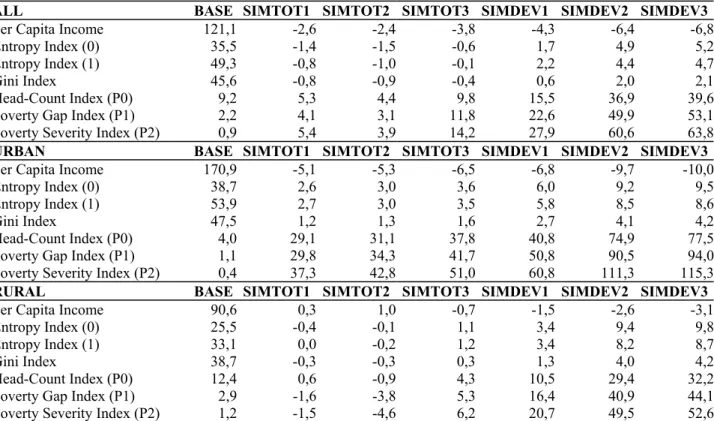
Table 1: Simulations ... 22

Table 2 : Macroeconomic simulation results ... 22

Table 3 : Microeconomic simulation results with full microsimulation model (FULL)... 22

Table 4 : Microeconomic simulation results with Representative Household Groups (RHG)... 23

List of graphs

Graph 1 :Terms of Trade Simulation Results without Reranking... 24

Graph 2: Terms of Trade Simulation Results with Reranking... 25

Graph 3 :Devaluation Simulation Results without Reranking ... 26

INTRODUCTION

There are various ways distributional issues might be analyzed within the framework of economy-wide models. The most common method relies on defining representative household groups (RHG) characterized by different combinations of factor endowments and possibly different labor supply, saving, and consumption behavior. The heterogeneity of the population of households is integrated into economy-wide or macro modelling through a two-way channel. In one direction, heterogeneity affects aggregate demand and labor supply and their structure in terms of goods and labor types. In the other direction, household income heterogeneity depends on the remuneration rates of the various factors of production, which are determined at the aggregate level.

The amount of heterogeneity that can be accounted for with this approach depends on the number of RHGs specified in the model. It is easier to work with a small number of groups because they can be more easily differentiated and the number of equations to deal with is smaller. To get closer to observed heterogeneity, it is then often assumed that each group results from the aggregation of households which are heterogeneous with respect to their preferences or the productivity of the factors they own. Practically, however, it is assumed that the distribution of relative income within a RHG follows some law that is completely exogenous. In general, this law is estimated on the basis of household surveys where the same groups as in the macro model may be identified2_{. This specification permits making the distribution of income}

“predicted” or simulated with the model closer to actual distribution data. It remains true, however, that the inequality being modelled in counterfactual analyses essentially is the inequality “between” representative groups.

From a conceptual point of view, the difficulty with this approach is that the assumption of exogenous within-group income heterogeneity is essentially ad hoc. If households within a group are different, why would their differences be independent of macroeconomic events? From an empirical point of view, the problem is that observed changes in income distribution are such that changes in within-group inequality generally are at least as important as changes in between-group inequality3_.

An example may help understand the nature of the difficulty. Suppose that a sizable proportion of households in a country obtain income from various sources—wage work in the formal or informal sector, farm income, other self-employment income—as is common in many developing countries, especially in Asia. If RHGs are defined, as is usually done, by the sector of activity and the employment status of the head (small farmers, urban unskilled workers in the formal sector, etc.), it does not seem difficult to take into account this multiplicity of income sources. When generating counterfactuals, however, two difficulties arise. First, imagine that the counterfactual drastically modifies the number of unskilled urban workers employed in the formal sector. What should be done with the number of households whose head is in that occupation? Should it be modified? If so, from which groups must new households in that RHG be taken or to which groups should they be allocated? Would it then be reasonable to assume that the distribution of income within each of these RHGs remains the same despite movements from one to the other? Second, assume that changes in occupation affect only secondary members and not household heads, so that weights of RHGs within the population are unchanged. Is it reasonable then to assume that all households in a group are affected in the same way by this change in the activity of some of their members? That a secondary member moves out of the formal sector back into family self-employment may happen only in a sub-group of households belonging to a given representative group. Yet, it may seriously affect the distribution within this group. While this kind of phenomenon may be behind the importance of the within-group component in decomposition exercises of changes in inequality, they are practically ignored in sector, multi-household RHG models.

2 _{For early applications of this type of model, see Adelman and Robinson (1978) and Dervis, de Melo and Robinson (1982), who specified}

lognormal within-group distributions with exogenous variances. The tradition is now well established—as may be seen in the surveys of CGE models for developing countries by Decaluwe and Martens (1987) and Robinson (1989). This approach may also distinguish among various income sources, in which case within-group variances and covariances must be exogenously specified--see Narayana et al. (1991).

3 _{Starting with Mookherjee and Shorroks' (1982) study of UK. There are now numerous examples of “within/between” decomposition analysis of}

changes in inequality leading to the same conclusion. Ahuja et al. (1998) illustrate this point very well for several Asian countries in the 1980s and 1990s.

What may be wrong in the preceding example is that RHGs are defined too precisely. Why look at urban unskilled workers in the formal sector, and not at urban unskilled workers in general? But if one looks at a broader group, despite the fact that wage differentials are observed between the formal and informal urban sectors, then the assumption of constant within-group distributions becomes untenable for any counterfactual that modifies the relative weights of the two sectors.

An obvious alternative approach, and a more direct way of dealing with distributional issues in macro modelling, would be to specify as many representative household groups as there are households in the population or in any available representative sample from the population. Computable general equilibrium (CGE) models based on observed rather than representative households do exist. But they usually concern a specific sector, a specific market, or a community—for example, CGE models of village economies4_.

Dealing with the whole economy and a representative sample of the whole population raises more difficulties5_{. The issue is not so much computational—computing simultaneous equilibrium in markets with}

thousands of independent agents is no longer very difficult. The real problem is that of identifying the heterogeneity of factor endowments or preferences at the level of a single household or individual.

Calibrating the consumption and labor supply behavior of a representative household is generally done by assuming some functional form for preferences and ignoring the underlying individual heterogeneity. Operating at the individual level requires dealing explicitly with that heterogeneity and introducing “fixed effects” to represent it. This is generally done by estimating a structural model on the observed cross-section of households and interpreting residuals as fixed individual effects. This estimation work usually involves identification assumptions which may be debatable, though. For instance, the estimation of the price elasticity of labor supply often calls for exclusion restrictions, and fixed effects behind the residuals of wage or labor supply equations are likely to reflect a very specific kind of preference or labor skill heterogeneity, together with measurement errors and other disturbances. Another difficulty is the complexity of structural models meant to represent satisfactorily household income generation behavior. This is true in particular when the modelling of the labor market requires accounting explicitly, as in the example above, for the joint labor supply behavior of individual household members. These two difficulties explain why micro-data-based applied general equilibrium models often rely on relatively simple structural models focusing on only one or two dimensions of household or individual behavior—see for instance Browning et al. (1999), Townsend and Ueda (2001), or Heckman (2001). Yet, it is not clear that this type of model may be convincingly used to describe the full complexity of household income inequality and the way it may be affected by macro-economic policies.

In this paper, we propose an alternative approach to quantify the effects of macro-economic shocks on poverty and inequality which tries to bypass the preceding difficulties. It combines a standard multi-sector CGE model with a micro-simulation model that describes real income generation behavior among a representative sample of households. This micro-simulation model is based on econometric reduced form equations for individual earnings, household income from self-employment, and the occupational choice of all household members of working age. Such an integrated set of equations has proved useful in analyzing observed changes in the distribution of income over some period of time in various countries—see Bourguignon et al. (2001) and the various papers in the MIDD project run by Bourguignon, Ferreira and Lustig6_{. It is used here to study changes between two hypothetical states of the economy as described by an}

economy-wide CGE model.

What makes the method proposed in this paper simpler than a fully integrated model with as many RHGs as actual households in a representative sample is that the two parts of the modelling structure are treated separately, in a top-down fashion. The macro or CGE model is solved first and communicates with the micro-simulation model through a vector of prices, wages, and aggregate employment variables. Then the micro-simulation model is used to generate changes in individual wages, self-employment incomes, and employment status in a way that is consistent with the set of macro variables generated by the macro model.

4 _{See for instance Taylor and Adelman (1996) for village models and Heckman (2001) for labor market applications.}

5 _{For attempts at the full integration of micro data and household income generation modeling within multi-sectoral general frameworks, see}

Cogneau (2001) and Cogneau and Robilliard (2001). A general discussion of the link between CGE modeling and micro-unit household data is provided by Plumb (2001).

When this is done, the full distribution of real household income corresponding to the shock or policy change initially simulated in the macro model may be evaluated.

For illustrative purposes, this framework is used to estimate the effects on the distribution of household income of various scenarios of real devaluation in Indonesia. The CGE part of this framework is fairly standard and could be replaced by any other macro model that could provide satisfactory counterfactuals for the variables that ensure the link with the micro-simulation model. For this reason, the presentation focuses more on the micro-simulation model than on the CGE model or the nature of the macro shock driving the simulations.

The paper is organized as follows. Section 1 shows the structure of the micro-simulation model and how it is linked to the CGE model. Section 2 describes the general features of the CGE model. The devaluation scenario and its implications for the distribution of household income are presented in Section 3. Finally, section 4 discusses the differences between the micro/macro framework proposed in this paper and the standard representative household group (RHG) approach.

1.

THE MICRO-SIMULATION MODEL

This section describes the specification of the household income model used for micro-simulation and then focuses on the way consistency between the micro-simulation model and the predictions of the CGE model is achieved. A detailed discussion of the specification and econometric estimates of the various equations of the household income generation model and simulation methodology may be found in Alatas and Bourguignon (2000)7_.

1.1.

The household income generation model

With the notation used in the rest of this paper, the household income generation model for household m and working age household members i = 1, .., km consists of the following set of equations:

( ) ( )

α

β

= + + mi g mi mi g mi mi Log w x v

i

=

1

,..

k

m ₍₁₎ ( ) ( ) ( )

γ

δ

λ

η

=

+

+

+

m f m m f m f m m m

Log y

Z

N

(2)       + > + =

∑

= m m m k i mi mi m m w IW y Ind N y P Y m ₀ 1 ) 0 ( 1 (3) 1 =

=

∑

K m mk k k

P

s p

(4) ( ) ( ) ( ) ( ) [ (0, )] = w + w + w > s + s + s mi h mi mi h mi mi h mi mi h mi mi IW Ind a z b u Sup a z b u (5) ( ) ( ) ( ) ( ) 1 [ (0, )] = =

∑

km s + s + s > w + w + w m h mi mi h mi mi h mi mi h mi mi i N Ind a z b u Sup a z b u (6)

The first equation expresses the logarithm of the (full-time) wage of member i of household m as a function of his/her personal characteristics, x. The residual term, vmi, describes the effects of unobserved earning

determinants and possibly measurement errors. This earning function is defined independently on various “segments” of the labor market defined by gender, skill (less than secondary or more than primary), and area (urban/rural). The function g() is an index function that indicates the labor market segment to which member i in household m belongs. Individual characteristics, x, thus permit representing the heterogeneity of earnings within wage earner groups due to differences in age, educational attainment within primary or secondary, and region. The second equation is the (net) income function associated with self-employment, or small

7 _{A more general discussion of the model may be found in Bourguignon, Ferreira and Lustig (1998) and Bourguignon, Fournier and Gurgand}

entrepreneurial activity, which includes both the opportunity cost of household labor and profit. This function is defined at the household level. It depends on the number Nm of household members actually

involved in that activity and on some household characteristics, Zm. The latter include area of residence, the

age and schooling of the household head, and land size for farmers. The residual term, ηm, summarizes the

effects of unobserved determinants of self-employment income. A different function is used depending on whether the household is involved in farm or non-farm activity. This is exogenous and defined by whether the household has access to land or not, as represented by the index function f(m).

The third equation is an accounting identity that defines total household real income, Ym, as the sum of the

wage income of its members, profit from self-employment, and (exogenous) non-labor income, y0m. In this

equation, the notation IWmi stands for a dummy variable that is equal to unity if member i is a wage worker

and zero otherwise. Thus wages are summed over only those members actually engaged in wage work. Note that it is implicitly assumed here that all wage workers are employed full-time. This assumption will be weakened later. Income from self-employment has to be taken into account only if there is at least one member of the household engaged in self-employment activity, that is if the indicator function, Ind, defined on the logical expression (Nm>0) is equal to unity. Total income is then deflated by a household specific

consumer price index, Pm, which is derived from the observed budget shares, smk, of household m and the

price, pk, of the various consumption goods, k, in the model (equation 4).

The last two equations represent the occupational choice made by household members. This choice is discrete. Each individual has to choose from three alternatives: being inactive, being a wage worker, or being self-employed. A fourth alternative consisting of being both self-employed and a wage worker is also taken into account but, for the sake of simplicity, it is ignored in what follows. Individuals chose among alternatives according to some criterion the value of which is specific to the alternative. The alternative with the highest criterion value is selected.

The criterion value associated with being inactive is arbitrarily set to zero, whereas the value of being a wage worker or self-employed are linear functions of a set of individual and household characteristics, zmi. The

intercept of these functions has a component, aw _{or a}s_{, that is common to all individuals and an idiosyncratic}

term, umi, which stands for unobserved determinants of occupational choices. The coefficients of individual

characteristics zmi, bw, or bs, are common to all individuals. However, they may differ across demographic

groups indexed by h(mi). For instance, occupational choice behavior, as described by coefficients aw_{, a}s_{, b}w

and bs _{and the variables in z}

mi may be different for household heads, spouses, male or female children. The

intercepts may also be demography specific.

Given this specification, an individual will prefer wage work if the value of the criterion associated with that activity is higher than that associated with the two other activities. This is the meaning of equation (5). Likewise, the number of employed workers in a household is the number of individuals for whom self-employment yields a criterion value higher than that of the two alternatives, as represented in (6)8_.

The model is now complete. Overall, it defines the total real income of a household as a non-linear function of the observed characteristics of household members (xmi and zmi), some characteristics of the household

(Zm), its budget shares (sm), and unobserved characteristics of the household (ηm) or household members (vmi,

uw

mi,and usmi). This function depends on five sets of parameters: the parameters in the earning functions (αg

and βg), for each labor market segment, g; the parameters of the self-employment income functions (γf, δf,

and λf) for the farm or non-farm sector, f; the parameters of the occupational choice model (awh, bwh, ash and

bsh), for the various demographic groups h, and the vector of prices (p). It will be seen below that it is

through a subset of these parameters that the results of the CGE part of the model may be transmitted to the micro-simulation module.

8 _{As mentioned above, the possibility that a person be involved simultaneously in wage work and self-employment is also considered. This is taken}

as an additional alternative in the discrete choice model (5). A dummy variable controls for this in the earning equation (1) and this person is

The micro-simulation model gives a complete description of household income generation mechanisms by focusing on both earning and occupational choice determinants. However, a number of assumptions about the functioning of the labor market are incorporated in this specification. The fact that labor supply is considered as a discrete choice between inactivity and full time work for wages or for self-employment income within the household calls for two sets of remarks. First, the assumption that individuals either are inactive or work full time is justified essentially by the fact that no information on working time is available in the micro data source used to estimate the model coefficients. Practically, this implies that estimated individual earning functions (1) and profit functions (2) may incorporate some labor supply dimension. Second, distinguishing between wage work and self-employment is implicitly equivalent to assuming that the Indonesian labor market is imperfectly competitive. If this were not the case, then returns to labor would be the same in both types of occupations and self-employment income would be different from outside wage income only because it would incorporate the returns to non-labor assets being used. The specification that has been selected is partly justified by the fact that assets used in self-employment are not observed, so that one cannot distinguish between self-employment income due to labor and that due to other assets. But it is also justified by the fact that the labor market may be segmented in the sense that labor returns are not equalized across wage work and self-employment. There may be various reasons for this segmentation. On the one hand, there may be rationing in the wage labor market. People unable to find a job as a wage worker move into self-employment, which thus appears as a kind of shelter. On the other hand, there may be externalities that make working within and outside the household imperfect substitutes. All these interpretations are fully consistent with the way in which the labor-market is represented in the CGE part of the model—see below9_.

1.2.

Estimation of the model for the benchmark simulation

The benchmark simulation of the model requires previous econometric estimation work. This is necessary to have an initial set of coefficients (αg, βg, γf, δf, λf, awh, bwh, ash, bsh) as well as an estimate of the unobserved

characteristics, or fixed effects, that enter the earning and profit functions, or the utility of the various occupational alternatives, through the residual terms (vmi, ηm, uwmi , usmi).

The data base consists of the sample of 9,800 households surveyed in the “income and saving” module of Indonesia's 1996 SUSENAS household survey. This sample is itself a sub-sample of the original 1996 SUSENAS. The coefficients of earning and self-employment income functions and the corresponding residual terms are obtained by ordinary least square estimation on wage earners and households with some self-employment activity10_{. This estimation also yields estimates of the residual terms, v}

mi and ηm. For

individuals at working age (i.e. 15 years and older) who are not observed as wage earners in the survey, unobserved characteristics, vmi, are generated by drawing random numbers from the distribution that is

observed for actual wage earners. The same is done with ηm for those households who are not observed as

self-employed in the survey but might get involved in that activity in a subsequent simulation11_.

Parameters of the occupational choice model were obtained through the estimation of a multi-logit model, thus assuming that the residual terms (uw

mi , usmi) are distributed according to the double exponential law. The

estimation was conducted on all individuals of working age, but separately for three demographic groups (h): household heads, spouses, and other family members. The set of explanatory variables, zmi, includes not only

the socio-demographic characteristics of the individual, but also the average characteristics of the other members in the household and the size and composition of the household. In addition, it includes the occupational status of the head, and possibly his/her individual earning, for spouses and other household members. For all individuals, values of the residual terms (uw

mi , usmi) were drawn randomly in a way

9 _{This “rationing” view at the labor market explains why we refrain from calling “utility” the criteria that describe occupational choices, as is}

usually done. Actually, the functions defined in (5)-(6) combine both utility aspects and the way in which the rationing scheme may depend on individual characteristics.

10 _{Correction for selection biases did not lead to significant changes in the coefficients of these equations and was thus dropped.}

consistent with observed occupational choices12_{. For instance, residual terms for a wage earner should be}

such that: ˆw_{( )} + ˆw_{( )}+ w > (0,ˆs_{( )}+ ˆs_{( )}+ s )

h mi mi h mi mi h mi mi h mi mi

a z b u Sup a z b u

where the ^ notation corresponds to multi-logit coefficient estimates13_.

To save space, the results of this estimation work are not reported in this paper. Interested readers may find a presentation and a discussion of a similar household income model in Alatas and Bourguignon (2000). Note that the CPI equation (4) does not call for any estimation since it is directly defined on observed household budget shares.

1.3.

Link with the CGE model

In principle, the link between the micro-simulation model that has just been described and the CGE model is extremely simple. It consists of associating macro-economic shocks and changes in policies simulated in the CGE model to changes in the set of coefficients of the household income generation model (1)-(6). With a new set of coefficients (αg, βg, γf, δf, λf, awh, bwh, ash, bsh) and the observed and unobserved individual and

household characteristics (xmi, zmi, Zm, sm, vmi, ηm, uwmi , usmi), these equations permit computing the

occupational status of all household members, their earnings, self-employment income, and finally total real income of the household. But this association has to be done in a consistent way. Consistency with the equilibrium of aggregate markets in the CGE model requires that: (1) changes in average earnings with respect to the benchmark in the micro-simulation must be equal to changes in wage rates obtained in the CGE model for each segment of the wage labor market; (2) changes in self-employment income in the micro-simulation must be equal to changes in informal sector income per worker in the CGE model; (3) changes in the number of wage workers and self-employed by labor-market segment in the micro-simulation model must match those same changes in the CGE model, and (4) changes in the consumption price vector, p, must be consistent with the CGE model.

The calibration of the CGE model, or of the Social Accounting Matrix behind it, is done in such a way that the preceding four sets of consistency requirements are satisfied in the benchmark simulation. Let EG be the

employment level in the G segment of the wage labor market, wG the corresponding wage rate, SG the

number of self-employed in the same segment and IF the total self-employment household income in

informal sector F (farm and non-farm). Finally, let q be the vector of prices for consumption goods in the CGE model. Consistency between the micro data base and the benchmark run of the CGE model is described by the following set of constraints:

( ) ( ) ( ) ( ) , ( ) ( ) ( ) ( ) ( ) , ( ) ( ) ˆ ˆ ˆ ˆ ˆ ˆ [ . (0, . ) ] ˆ ˆ ˆ ˆ ˆ ˆ [ . (0, . ) ] ˆ ˆ ˆ ˆ ( . ). [ w w w s s s h mi mi h mi mi h mi mi h mi mi G m i g mi G S S S w w w h mi mi h mi mi h mi mi h mi mi G m i g mi G w G mi G mi h mi Ind a z b u Sup a z b u E Ind a z b u Sup a z b u S Expα x β v Ind a z = = + + > + + = + + > + + = + + +

∑ ∑

∑ ∑

( ) ( ) ( ) , ( ) , ( ) ( ) ( ) ( ) ( ) ˆ _{ˆ ˆ} ˆ _ˆ . (0, . ) ] ˆ ˆ ˆ ˆ ˆ ( . . ). ( 0) ˆ ˆ ˆ _{[ˆ . ˆ (0, ˆ . ˆ ) ]} w w s s s mi h mi mi h mi mi h mi mi G m i g mi G F m F F m m m F m f m F S S S w w w m h mi mi h mi mi h mi mi h mi mi i b u Sup a z b u w Exp Z N Ind N I

with N Ind a z b u Sup a z b u

γ δ λ η = = + > + + = + + + > = = + + > + +

∑ ∑

∑

∑

for all labor-market segments, G, and both self-employment sectors, F.

12 _{In general, the residual terms in the occupational functions (u}w

mi , usmi) should be assumed to be correlated with the residual terms of the earning

and self-employment income functions (vmi, ηm). Failure to find significant self-selection correction terms in the latter equations suggest this

correlation is negligible, however.

13 _{This may be done by drawing (u}w

mi , usmi) independently in double exponential laws until they satisfy the preceding condition. A more direct

In these equations, the ^ notation refers to the results of the estimation procedure described above. Given the way in which the unobserved characteristics or fixed effects (vmi, ηm, uwmi , usmi) have been generated,

predicted occupational choices, earnings, and self-employment income that appear in these equations are identical to those actually observed in the micro data base for all households and individuals.

Consider now a shock or a policy measure in the CGE model which changes the vector (EG, SG, wG, IF, q)

into (E*

G, S*G, w*G, I*F, q*). The consistency problem is to find a new set of parameters C = (αg, βg, γf, δf, λf,

aw

h, bwh, ash, bsh, p) of the micro-simulation model such that the preceding set of constraints will continue to

hold for the new set of right hand macro variables (E*_{G, S}*_{G, w}*_{G, I}*_{F, q*). This is trivial for consumption} prices, p, which must be equal to their CGE counterpart. For the other parameters, there are many such sets of coefficients so that additional restrictions are necessary. The choice made in this paper is to restrict the changes in C to changes in the intercepts of all earning, self-employment income, and occupational criterion functions—that is changes in αg_{, γ}f_{, a}w

h and ash.

The justification for that choice is that it implies a “neutrality” of the changes being made with respect to individual or household characteristics. For example, changing the intercepts of the log earning equations generates a proportional change of all earnings in a labor-market segment, irrespectively of individual characteristics—outside those that define the labor-market segments, that is skill, gender, and area. The same is true of the change in the intercept of the log self-employment income functions. It turns out that a similar argument applies to the criteria associated with the various occupational choices. Indeed, it is easily shown that changing the intercepts of the multi-logit model implies the following neutrality property. The relative change in the ex-ante probability that an individual has some occupation depends only on the initial ex-ante probabilities of the various occupational choices, rather than on individual characteristics.

More precisely, let

_,

_and

0

mi s

mi w

mi

P

P

P

be the a priori probabilities of wage work, self-employment and no employment for individual mi. According to the multi-logit model, these probabilities have the following expression14_:

)

(

)

(

1

)

(

,

)

(

)

(

1

)

(

s mi s w mi w w mi w s mi s mi s w mi w w mi w w mi

b

z

a

Exp

b

z

a

Exp

b

z

a

Exp

P

b

z

a

Exp

b

z

a

Exp

b

z

a

Exp

P

+

+

+

+

+

=

+

+

+

+

+

=

(7) and mis w mi mi

P

P

P

0

= 1

−

−

. Then, differentiating with respect to the intercepts yields the preceding property, namely: w mi w mi mi w s mi s mi w mi w w mi w mi

_P

da

P

dP

da

P

dP

P

da

P

dP

−

=

=

−

=

.

.

,

)

1

(

.

0 0 (8) and symmetrically for

a

s.

14 _{The following argument is cast in terms of ex-ante probabilities of the various occupation rather than the actual occupational choice that appear in}

the preceding system of equation. This is for the sake of simplicity. Note that ex-ante probabilities given by the multi-logit model correspond to the observed frequency of occupation among individuals with the same observed characteristics. Also note that, for simplicity, we ignore demographic group heterogeneity h(mi) in what follows.

There are as many intercepts as there are constraints in the preceding system. Thus, the linkage between the CGE part of the model and the micro-simulation part is obtained through the resolution of the following system of equations: * * * ( ) ( ) ( ) ( ) , ( ) * * * ( ) ( ) ( ) ( ) , ( ) * * ( ) ˆ _ˆ ˆ _ˆ [ (0, )] ˆ _ˆ ˆ _ˆ [ (0, )] ˆ ˆ _ˆ (

α

β

) [ = = + + > + + = + + > + + = + + +

∑ ∑

∑ ∑

G G G w w w s s s h mi mi h mi mi h mi mi h mi mi m i g mi G S S S w w w h mi mi h mi mi h mi mi h mi mi m i g mi G w mi G mi h mi mi Ind a z b u Sup a z b u E Ind a z b u Sup a z b u S Exp x v Ind a z b * * ( ) ( ) ( ) , ( ) * * , ( ) * * * ( ) ( ) ( ) ( ) ˆ ˆ (0, ˆ )] ( ) ˆ ˆ ˆ _ˆ ( ) ( 0) ˆ ˆ ˆ _{[ ˆ (0, ˆ )]}

γ

δ

λ

η

= = + > + + = + + + > = = + + > + +

∑ ∑

∑

∑

G F F w w s s s h mi mi h mi mi h mi mi m i g mi G m F F m m m m f m F S S S w w w m h mi mi h mi mi h mi mi h mi mi i u Sup a z b u w S Exp Z N Ind N I

with N Ind a z b u Sup a z b u

for all labor-market segments, G, and both self-employment sectors, F. The unknowns of this system are αg*,

γf*, aw*h and as*h. There are as many equations as unknowns15. No formal proof of existence or uniqueness has

yet been established. But there is a strong presumption that these properties hold. Indeed, the last two sets of equations in αg*, γf* are independent of the first two sets and clearly have a unique solution for given values

of aw*

h and as*h since left hand sides are monotone functions that vary between zero and infinity. Things are

more difficult for the first two sets of equations, in particular because of the discreteness of the Ind( ) functions. If there are enough observations, these functions may be replaced by the probability to be in wage work or self-employed as given by the well-known multi-logit model. This would make the problem continuous. It can then be checked that local concavity properties make standard Gauss-Newton techniques convergent. However, the minimum number of observations necessary for the multi-logit probability approximation to be satisfactory is not clear16_.

Once the solution is obtained, it is a simple matter to compute the new income of each household in the sample, according to model (1)-(6), with the new set of coefficients αg*, γf*, aw*h and as*h and then to analyze

the modification that this implies for the overall distribution of income.

In the Indonesian case, the number of variables that allow the micro and the macro parts of the overall model to communicate, that is the vector (E*

G, S*G, w*G, I*F, q*), is equal to 26 plus the number of consumption

goods used in defining the household specific CPI deflator. There are 8 segments in the labor market. The employment requirements for each segment in the formal (wage work) and the informal (self-employment) sectors (E*

G and S*G) lead to 16 restrictions. In addition there are 8 wage rates in the formal sector (w*G) and

2 levels of self-employment income (I*

F) in the farm and non-farm sectors. Thus, simulated changes in the

distribution of income implied by the CGE part of the model are obtained through a procedure that comprises a rather sizable number of degrees of freedom.

1.4.

Interpretation of the consistency system of equations

The micro-macro linkage described by the preceding system of equations may be seen as a generalization of familiar grossing up operations aimed at correcting a household survey to make it consistent with other data sources—e.g. another survey or a census or national accounts. The first type of operation consists of simply rescaling the various household income sources, with a scaling factor that varies across the income sources and labor-market segments. This corresponds to the last two set of equations in the consistency system (S). However, because households may derive income from many different sources, this operation is more complex and has more subtle effects on the overall distribution than simply multiplying the total income of households whose head belongs to different groups by different proportionality factors, as is often done. It is

15 _{Of course, this requires some particular relationship between the number of demographic groups, h, and the number of labor-market segments, G.}

also worth stressing that, because various labor segments are distinguished by gender, area, and skill, changing the intercepts of the various wage equations model is actually equivalent to making the coefficients of education, gender, or area of residence in a single wage earning function endogenous and consistent with the CGE model. The second operation would consist of reweighing households depending on the occupation of their members17_{. This approach loosely corresponds to the first two sets of restrictions in system (S). Here}

again, however, this procedure is considerably different from reweighing households on the basis of a simple criterion like the occupation of the household head, his/her education, or area of residence. There are two reasons for this. First, reweighing takes place on individuals rather than households, so that the composition of households and the occupation of their members matter. Second, the reweighing being implemented is highly selective. For instance, if the CGE model results require that many individuals move from wage work to self-employment and inactivity, individuals whose occupational status will change in the micro-simulation model will not be drawn randomly from the initial population of individuals in the formal sector. On the contrary, they will be drawn in a selective way, essentially based on cross-sectional estimates of their a priori probability of being a formal wage worker or self-employed. Standard reweighing would consist of modifying these ex-ante probabilities of being a formal wage worker, w

mi

P

, in the same proportion. The selective reweighing used here is such that this proportion depends itself on the ex-ante probabilities of being a wage worker, as shown by equations (8). For instance, the youngest employees in a household with many employees, but with self-employed parents, might be more likely to move than an older person in a small household. As the earnings or the income of the former may be different from that of the latter, this selectivity of the reweighing procedure has a direct effect on the distribution of earnings within the group of formal wage workers.

1.5.

Interpreting the intercepts of occupational choice criteria

There is another way of interpreting this reweighing procedure, or the changes in the multi-logit intercepts which it relies on, that can be made consistent with standard utility maximizing behavior, and with the CGE part of the whole model.

Consider that each occupation yields some utility that can be measured by the log of the money income it yields, net of working disutility. To simplify, ignore momentarily the distinction between individuals and households and write the utility of the three occupations with obvious notations as:

)

(

)

(

)

(

)

(

)

(

)

(

0 0 0 i i i i i s i i s i i s i w i i w i i w i

z

p

CPI

Log

Y

Log

U

z

p

CPI

Log

y

Log

U

z

p

CPI

Log

w

Log

U

µ

φ

µ

φ

µ

ϕ

+

−

−

=

+

−

−

=

+

−

−

=

(9)

where Yi is the monetary equivalent of domestic production in case of no employment. In all these cases, the first two terms on the RHS corresponds to the (log) of the real (or real equivalent) return to each occupation, and the third term to the disutility of that occupation. This disutility is itself expressed as a linear function of individual or household characteristics, zi, and a random term, µi. Of course, such a specification of the

indirect utility function presupposes some separability between consumption and the disutility of occupations in the direct utility function18_.

17 _{For simulation techniques of income or earnings distribution based on straight reweighing of a benchmark sample see diNardo, Fortin, Lemieux}

(1996).

18 _{A direct utility function of the type U}

i(c,l;zi) = Log[ai(c)]-b(l,zi), where ai(c,z) is a linearly homogeneous function of the consumption vector , c,

This specification permits putting more economic structure into the initial specification of the multi-logit model for occupational choices. In particular, it is possible to replace Log(wi) and Log(yi) by their expression

in (1) and (2). In addition, we know that the intercept of the earning function depends on the earning of the labor-market segment an individual belongs to, as given by the CGE model. Likewise, the intercept of the self-employment income function depends on the value-added price of the output of self-employment activity, and therefore on the whole price vector as given by the CGE model. Of course, the same can be said of the unobserved domestic output, Yi, in case of inactivity. Thus the income terms in (9) may be rewritten

as: i i i i i f i i f i i i G i i G i z p Y Log z p y Log v z w w Log

ζ

λ

χ

η

δ

γ

β

α

+ + = + + = + + = . ) ( . ) ( . ) ( ) ( ) ( ) ( ) ( (10)

where wG and p are earnings and prices given by the CGE model. Combining (9) and (10) i finally leads to

the equivalent of the multi-logit formulation (5)-(6). Using inactivity as the default choice permits eliminating the heterogeneity in consumption preferences associated with specific CPI indices, CPIi(p). The preferred occupational choice of individual i, Ci, belonging to labor market segment G, is wage work, W, self-employment, S, or inactivity I, is then given by a conditional system with the following structure:

[

]

[

]

[

(

)

.

,

(

,

)

.

]

0

.

)

,

(

,

0

.

)

(

.

)

(

,

0

.

)

,

(

) ( ) ( ) ( ) ( ) ( ) ( ) (

<

+

+

+

+

=

+

+

≥

+

+

=

+

+

≥

+

+

=

w i G w i i G w s s i s i w i G w i i G w s s i s i s i G s i s w i G w i i G i i i i i i i w

B

z

p

w

A

B

z

p

A

Sup

if

I

C

B

z

p

w

A

Sup

B

z

p

A

if

S

C

B

z

p

A

Sup

B

z

p

w

A

if

W

C

ω

ω

ω

ω

ω

ω

If the functionsA (w_G(i),p) andA_s(p)

w were known, we would have a complete micro-economic structural

labor supply model that could nicely fit into the CGE model. Given a wage-price vector (w,p), this model would give the occupational choice of every individual in sample and therefore labor supply in the CGE. It would then be possible to have the whole micro-simulation structure integrated within the CGE model. The fundamental point, however, is that there is no way we can get an estimate of these functions on a micro-economic cross-sectional basis, for there is no variation of the price vector, p, in the data. If we do not want to import the functions A (w_G(i),p) andA_s(p)

w arbitrarily from outside the micro-simulation framework

and household survey data, the only way to achieve consistency with the CGE part of the model is to assume that these functions are such that the equilibrium values of wages and prices coming from the CGE model ensure the equilibrium of markets for both goods and labor. This is equivalent to looking for the intercepts that ensure supply demand equilibrium of the labor markets behind the last two sets of equations of system (S).Solving system (S) for those intercepts thus is consistent, under the preceding assumptions above, with the full general equilibrium of the economy and full utility-maximizing behavior at the micro-level. It is a solution that permits avoiding arbitrary assumptions necessary to get a structural representation of individual labor choices explicitly consistent with the CGE model.

It must be kept in mind that the preceding argument has been conducted in terms of the textbook consumption unit, rather than individuals belonging to the same household, as explicitly stated in the micro-simulation model (1)-(6). Interpreting the occupational status equations in terms of rational individual behavior would thus require specifying some intra-household task/consumption allocation model. Because of the cross-wage elasticities of occupational choices, it is not clear, in particular, that the standard unitary model is consistent with the idea that all price and wage effects in the micro-simulation model are included in the intercepts of the multi-logit criterion functions. Justifying that assumption may require invoking some non-unitary model of household decision, but this point was not investigated further. All the preceding discussion is based on a purely competitive view of the labor market. But the occupational model represented by equation (5)-(6) may be justified by other arguments, for instance by the existence of selective rationing. This would seem natural in view of the imperfection assumed for the labor markets in the CGE—see below. Most of the preceding conclusions would still hold, however. Maintaining the maximum dichotomy between the micro and the macro part of the model requires avoiding the import of structural assumptions from

outside the micro-economic model. At the same time, insuring consistency through the intercepts simplifies things but also imposes implicit assumptions that one would like to identify more precisely.

The lack of communication between the macro and the micro part of the model is also concerned with the non-labor income variable, y0m. It is taken as exogenous (in nominal terms) in all simulations. Yet, it includes

housing and land rents, dividends, royalties, imputed rents from self-occupied housing, and transfers from other households and institutions. It could have been possible to endogenize some of these items in the CGE model, but this was not done.

2.

THE CGE MODEL

The macro model used in this paper is a conventional, trade-focused CGE model19_{. It is based on a Social}

Accounting Matrix (SAM) for the year 1995. The SAM has been disaggregated using cross-entropy estimation methods (Robinson, Cattaneo, and El-Said, 2001) and includes 38 sectors (“activities”), 14 goods (“commodities”), 14 factors of production (8 labor categories and 6 types of capital), and 10 households types, as well as the usual accounts for aggregate agents (firms, government, rest of the world, and savings-investment). The CGE model starts from the standard neoclassical specification in Dervis et al. (1982), but it also incorporates disaggregation of production sectors into formal and informal activities and associated labor-market imperfections, as well as working capital. The SAM, including the sector and agent breakdown, is given in Appendix A.

The model is Walrasian in the sense that it determines only relative prices, and other endogenous real variables in the economy. Financial mechanisms are modelled implicitly and only their real effects are taken into account in a simplified way. Sectoral product prices and factor prices are defined relatively to the producer price index of goods for domestic use, which serves as the numeraire.

In common with many trade-focused CGE models, the model includes an explicit exchange-rate variable. Since world prices are measured in U.S. dollars and domestic prices in Indonesian currency, the exchange-rate variable has units of domestic currency per unit of foreign exchange—it is used to convert world prices of imports and exports to prices in domestic currency units, and also to convert foreign-exchange flows measured in dollars (e.g., foreign savings). Given the choice of numeraire, the exchange rate variable can be interpreted as the real price-level-deflated (PLD) exchange rate, deflating by the domestic (producer) price of non-traded goods20_{. Since world prices are assumed fixed, the exchange rate variable corresponds to the real}

exchange rate, measuring the relative price of traded goods (both exports and imports) and nontraded goods. Following Armington (1969), the model assumes imperfect substitutability for each good between the domestic commodity—which results itself from a combination of formal and informal activities—and imports. What is demanded is a composite good, which is a CES aggregation of imports and domestically produced goods. For export commodities, the allocation of domestic output between exports and domestic sales is determined on the assumption that domestic producers maximize profits subject to imperfect transformability between these two alternatives. The composite production good is a CET (constant-elasticity-of-transformation) aggregation of sectoral exports and domestically consumed products21_.

Indonesia’s economy is dualistic, which the model captures by distinguishing between formal and informal “activities” in each sector. Both sub-sectors produce the same “commodity” but differ in the type of factors they use22_{. This distinction allows treating formal and informal factor markets differently. On the demand}

side, imperfect substitutability is assumed between formal and informal products of the same commodity classification.

19 _{For a detailed exposition of this type of model, and for the implementation of the “standard” model in the GAMS modeling language, see Lofgren}

et al. (2001).

20 _{This terminology was standardized in a series of NBER studies in the 1970s in a project led by Jagdish Bhagwati and Anne Krueger.}

21 _{The appropriate definition of the real exchange rate in this class of model, with a continuum of substitutability between domestically produced}

and foreign goods, is discussed in Devarajan, Lewis and Robinson (1993).

22 _{Typically, CGE models assume a one-to-one correspondance between activities and commodities. This model allows many activities producing}

For all activities, the production technology is represented by a set of nested CES (constant-elasticity-of-substitution) value-added functions and fixed (Leontief) intermediate input coefficients. Domestic prices of commodities are flexible, varying to clear markets in a competitive setting where individual suppliers and demanders are price-takers.

2.1.

Factors of Production

There are eight labor categories: Urban Male Unskilled, Urban Male Skilled, Urban Female Unskilled, Urban Female Skilled, Rural Male Unskilled, Rural Male Skilled, Rural Female Unskilled, and Rural Female Skilled. Male and female, as well as skilled and unskilled labor are assumed to be imperfect substitutes in the production activities.

In addition, labor markets are assumed to be segmented between formal and informal sectors. In the formal sectors, a degree of imperfect competition is assumed to result in there being an increasing wage-employment curve, and real wages are defined by the intersection of that curve with competitive labor demand. Informal sector labor is equivalent to self-employment. Wages in that sector are set so as to absorb all the labor not employed in the formal sectors. Non-wage income results from the other factors operated by self-employed.

Land appears as a factor of production in all agricultural sectors. Only one type of land is considered in the model. It is competitively allocated among the different crops and sectors so that its marginal revenue product is equated across all uses. Capital is broken down into six categories, but, given the short-run nature of the model, it is assumed to be fixed in each activity.

2.2.

Households

The disaggregation of households in the CGE model is not central for our purpose since changes in factor prices are passed on directly to the micro-simulation model, without use of the representative household groups (RHG) used in the original SAM and in the CGE model. Yet, this feature will later permit comparing the methodology developed in this paper with the standard CGE/RHG approach. Thus RHGs are endowed with some specific combination of factors (labor and capital) and derive income from the remuneration of these factors, which they supply in fixed quantity to the rest of the economy. Consumption demand by households is specified as a linear expenditure system (LES), with fixed marginal budget shares and minimum consumption (subsistence) level for each commodity.

2.3.

Macro Closure Rules

Aside from the supply-demand balances in product and factor markets, three macroeconomic balances must hold in the model: (i) the external trade balance (in goods and non-factor services), which implicitly equates the supply and demand for foreign exchange flows; (ii) savings-investment balance; and (iii) the fiscal balance, with government savings equal to the difference between government revenue and spending. As far as foreign exchange is concerned, foreign savings are taken as exogenous and the exchange rate is assumed to clear the market—the model solves for an equilibrium real exchange rate given the fixed trade balance. Concerning the last two constraints, three alternative closures will be considered in what follows. The objective behind these three macro-economic closures is to see whether they may affect the nature of the results obtained with the micro-simulation model and how they compare with those obtained with the RHG method.

The first macro closure assumes that aggregate investment and government spending are in fixed proportions to total absorption. Any shock affecting total absorption is thus assumed to be shared evenly among government spending, aggregate investment, and aggregate private consumption. While simple, this “balanced” closure effectively assumes a “successful” structural adjustment program whereby a macro shock is assumed not to cause particular actors—government, consumers, and industry—to bear a disproportionate share of the adjustment burden. This closure implies that the fiscal balance is endogenous.

In the second macro closure, investment is savings-driven and government spending adjusts to maintain the fiscal balance at the same level as in the benchmark simulation, which fits the economic situation observed

in 1997. Note, however, that government employment remains constant. The third macro closure achieves the same fiscal balance through a uniform increase in indirect (VAT) tax rates23_.

3.

SCENARIOS AND SIMULATION RESULTS

As the purpose of this section is essentially to illustrate empirically the way the micro-simulation model is linked with the CGE model, the nature of the shock being simulated does not matter very much. A companion paper uses an extended version of the model to describe the dramatic crisis that hit Indonesia in 199824_{. Two simpler scenarios are considered here—see table 1. They allow some foreign sector parameters}

to vary under the three alternative macro-economic closures listed above.

The first scenario consists of a major terms of trade shock that reduces the foreign price of both crude oil and exports of processed oil products—amounting altogether to approximately 40 per cent of total Indonesian exports—by 50 percent. The corresponding drop in foreign exchange receipts results in a devaluation of the equilibrium exchange rate (in order to increase exports and reduce imports) to maintain the fixed trade balance, under the three macro-economic adjustment scenarios described above. The corresponding simulations appear respectively under the headings SIMTOT1 to SIMTOT3 in the tables below.

The second scenario consists of a 30 percent drop in exogenous foreign savings. This shock also results in a devaluation, under the same three macro-economic adjustment scenarios as above. The corresponding simulations are referred to as SIMDEV1 to SIMDEV3. The main difference with the first set of simulations is that there is no change in relative prices before the devaluation, whereas the terms of trade shock in SIMTOT first reduces the relative prices of oil and oil products, both on the export and import sides, with spillover on the structure of domestic prices.

Table 2 shows the effects of these shocks on some macro-economic indicators. Results are unsurprising. GDP is little affected since both capital and the various types of labor are assumed to be fully employed. The small drop that is observed corresponds to sectoral shifts and price index effects. The effect of SIMTOT on the exchange rate and the volume of foreign trade is much less pronounced than that of SIMDEV. This result reflects the relative sizes of both shocks. In both cases, the resulting change in relative prices leads to an increase in the relative price of food products, which are largely non-traded. In turn, this causes an absolute increase in the real income of farmers that contrasts with the drop in the real income of self-employed in the urban sector and of all workers. With no change in the wage curve and a drop in labor demand coming from traded good sectors, which are the main employers of wage labor, wages fall. The drop is more pronounced for unskilled workers, reflecting more exposure to foreign competition by the sectors employing them. All these effects depend on the size of the devaluation, and are bigger in SIMDEV.

As far as the three macro-economic closures are concerned, it may be seen in table 2 that they make a difference only in the case of the foreign saving shock, SIMDEV. The last two closures lead to more intense sectoral reallocations due to the change in the structure of absorption and the composition of aggregate demand. This effect is slightly bigger with the last closure where the fiscal balance is re-established through a uniform change in VAT rates. Because the VAT affects the various sectors in different proportions, with exemptions for informal sectors, the sectoral shift in aggregate demand is more important. Changes in the relative remuneration of the various types of labor are also more pronounced under the last two closures in the pure devaluation scenario. These effects are practically absent in the terms-of-trade scenario because all sectoral shifts are dominated by the initial change in foreign prices.

Table 3 shows the effect of the simulated shocks on the distribution of income after feeding the micro-simulation model with values for the linkage variables provided by the CGE counterfactuals. Overall, the distributional effects of the terms-of-trade shock as reflected in standard summary inequality and poverty measures are limited. Inequality tends to go down, but the change in inequality measures shown in the table

23 _{The Indonesian CGE model includes other features, including demand for working capital in all sectors. These features have not been discussed}

here because no use is made of them in the experiments we report. See Robilliard et al. (2001) for a discussion of how the model was extended to capture the impact of the Asian financial crisis. See also Aziz and Thorbecke (2001).