Université Paris-Dauphine
École Doctorale de Dauphine
UNE APPROCHE MATHÉMATIQUE
DE L’IMAGERIE OPTIQUE
PAR COLORANT POTENTIOMÉTRIQUE
A Signal Processing Approach
to Voltage-Sensitive Dye Optical Imaging
THÈSE
Pour l’obtention du titre de
Docteur en Sciences
Spécialité Mathématiques Appliquées
Présentée par
Hugo RAGUET
Soutenue publiquement le 22 septembre 2014 devant le jury composé de
Dirk Jancke Ruhr-Universität Bochum Rapporteur
Jean-Christophe Pesquet Université Paris-Est Marne-la-Vallée Rapporteur
Frédéric Chavane Institut de Neurosciences de la Timone Examinateur
Laurent Cohen Université Paris-Dauphine Examinateur
Bertrand Thirion INRIA Examinateur
Dimitri Van De Ville Université de Genève Examinateur
Gabriel Peyré CNRS, Université Paris-Dauphine Directeur
Yves Frégnac CNRS Co-directeur
Résumé
L’imagerie optique par colorant potentiométrique est une méthode d’enregistrement de l’activité corticale prometteuse, mais dont le potentiel réel est limité par la présence d’artefacts et d’interférences dans les acquisitions. À partir de modèles existant dans la littérature, nous proposons un modèle génératif du signal basé sur un mélange additif de composantes, chacune contrainte dans une union d’espaces linéaires déterminés par son origine biophysique. Motivés par le problème de séparation de composantes qui en découle, qui est un problème inverse linéaire sous-déterminé, nous développons : (1) des régularisations convexes structurées spatialement, favorisant en particulier des solutions parcimonieuses ; (2) un nouvel algorithme proximal de premier ordre pour minimiser efficacement la fonctionnelle qui en résulte ; (3) des méthodes statistiques de sélection de paramètre basées sur l’estimateur non biaisé du risque de Stein. Nous étudions ces outils dans un cadre général, et discutons leur utilité pour de nombreux domaines des mathématiques appliqués, en particulier pour les problèmes inverses ou de régression en grande dimension. Nous développons par la suite un logiciel de sépa-ration de composantes en présence de bruit, dans un environnement intégré adapté à l’imagerie optique par colorant potentiométrique. Finalement, nous évaluons ce logiciel sur différentes données, synthétiques et réelles, montrant des résultats encourageants quant à la possibilité d’observer des dynamiques corticales complexes.
Mots-clés :imagerie optique par colorant potentiométrique, problème inverse, sépara-tion de composantes, parcimonie structurée, optimisasépara-tion convexe, méthode proximale, estimation du risque, sélection de paramètre.
Abstract
Voltage-sensitive dye optical imaging is a promising recording modality for the cor-tical activity, but its praccor-tical potential is limited by many artefacts and interferences in the acquisitions. Inspired by existing models in the literature, we propose a gen-erative model of the signal, based on an additive mixtures of components, each one being constrained within an union of linear spaces, determined by its biophysical ori-gin. Motivated by the resulting component separation problem, which is an underde-termined linear inverse problem, we develop: (1) convex, spatially structured regular-izations, enforcing in particular sparsity on the solutions; (2) a new first-order proximal algorithm for minimizing efficiently the resulting functional; (3) statistical methods for automatic parameters selection, based on Stein’s unbiased risk estimate. We study those methods in a general framework, and discuss their potential applications in various fields of applied mathematics, in particular for large scale inverse problems or regres-sions. We develop subsequently a software for noisy component separation, in an inte-grated environment adapted to voltage-sensitive dye optical imaging. Finally, we eval-uate this software on different data set, including synthetic and real data, showing en-couraging perspectives for the observation of complex cortical dynamics.
Keywords:voltage-sensitive dye optical imaging, inverse problem, component separa-tion, structured sparsity, convex optimizasepara-tion, proximal method, risk estimasepara-tion, pa-rameter selection.
Table of C ontents
Introduction 7
I VSDOI: Ways and Customs 21
1 Monitoring Cortical Activity with VSDOI . . . 22
2 The Challenge of VSDOI in vivo . . . 28
3 VSDOI Denoising: Previous Approaches . . . 30
Appendix. . . 38
References . . . 38
II Sparse Morphological Component Separation for VSDOI 43 1 Preliminary Notations . . . 44
2 The Model . . . 46
3 Spatially Structured Penalizations . . . 49
4 Discussion . . . 54
References . . . 55
III A Generalized Forward-Backward Splitting Algorithm 57 1 Monotone Inclusion and Minimization Problems . . . 58
2 Generalized Forward-Backward Splitting. . . 63
3 Convergence Proofs . . . 69
4 Conclusion and Perspectives . . . 76
References . . . 76
IV Splitting Spatially Structured Penalizations for Signal Processing 79 1 Norms and Sets in a Structured Euclidean Space . . . 80
2 Yet Another Discrete Total Variation Semi-Norm . . . 88
3 Proximal Splitting for Signal Processing . . . 92
4 Efficient Implementation of Splitting Algorithms . . . 108
5 Illustration and Experiments . . . 113
References . . . 121
V Risk Estimation for Parameter Selection 125 1 Stein’s Unbiased Risk Estimate for Denoising . . . 126
2 Derivation for Some Proximity Operators . . . 130
3 Beyond Proximity Operators . . . 140
4 Numerical Experiments . . . 145
5 Risk Estimate Beyond Denoising . . . 154
Appendix. . . 154
References . . . 157
VI A Full Component Separation Method for VSDOI 159 1 Scaling Penalizations for Noisy Component Separation . . . 160
2 Component Approximations for Parameters Selection . . . 162
Appendix. . . 170
VII Exploration of VSDOI With SMCS 171 1 Fluorescence, Gain, Noise. . . 173
2 Synthetic Data . . . 175
3 Orientation Selectivity in the Cat’s Visual Cortex . . . 184
4 Propagations in the Mouse’s Somatosensory Cortex . . . 194
5 Discussion and Perspectives . . . 196
Appendix. . . 199
References . . . 201
Conclusion 203
Introduction
A Signal Processing Approach
to Voltage-Sensitive Dye Optical Imaging
Voltage-sensitive dye optical imaging (VSDOI) is a recording modality of the corti-cal neuronal activity which is very promising for understanding the low-level sensory processing, particularly in mammals. In principles, this modality allows to observe in-vivo entire neuronal networks operating, with a temporal precision in the order of the millisecond and a spatial precision in the order of tens of microns. To put it differently, it represents for neuroscientists the possibility to eventually link, within the same theo-retical framework, microscopic knowledge with macroscopic observations.
Unfortunately, the complexity of the experimental protocols, the presence of arti-facts and interferences in the acquisitions, and the current lack of knowledge on the nature of the observed signal are so many limitations to unleash the true potential of this method. However, since its introduction back in the eighties, VSDOI has been
un-der constant improvements, as reported byDavila et al. (1973);Grinvald et al. (1999);
Shoham et al. (1999); Grinvald and Hildesheim (2004); Frostig (2009); Chemla and Chavane (2010b);Peterka et al. (2011)and many others. Most of those improvements are technological, in the sense that they can be attributed to more accurate recording de-vices, more controlled experimental conditions, and chemical synthesis of better dyes, i.e. more adapted fluorescent molecules enabling optical measurement of neuronal ac-tivity.
Naturally, as VSDOI became more reliable, it gained in popularity, and has already been used extensively by neurobiologists for in-vivo functional studies of the cortex, in various experimental conditions and subjects, from the anesthetized rodent to the awake monkey. In order to cope with the exceptionally high level of noise in the record-ings, many authors developed, independently, their own methods for extracting the sig-nal of interest. As reviewed in this thesis, these are often ad-hoc methods, for their par-ticular experimental conditions and the specific phenomenon under investigation. In other words, the denoising process is often merged together with the biological analysis of the data which would shed light on a neuroscientific question raised a priori.
It is at the heart of this thesis to step back from the actual goal of VSDOI, that is understanding how information is processed within the cortex, in order to get a better understanding of the signal itself, and confront VSDOI data to the most recent advances in mathematical theories of signal processing.
Outline
This work is a collaboration between the image processing team of Gabriel Peyré from the research center CEREMADE (Université Paris-Dauphine, France), and the neuroscience team of Yves Frégnac from the laboratory UNIC (Gif-sur-Yvette, France). The investigation of VSDOI was primarily possible thanks to Cyril Monier at UNIC, and later thanks to Isabelle Ferezou. We also collaborated with another experimentalist, Esin Yavuz, while she was working on her Ph.D. thesis at UNIC. Let us mention here that she also developed a method of signal processing for VSDOI, but from a different and complementary perspective from ours, since she was investigating specific functional
properties within the cat’s visual cortex (Yavuz, 2012).
This collaboration leads us to work on disparate domains. Because of this interdisci-plinarity, the chapters of this thesis are intended to be as independent as possible; though they are all linked by the main objective: developing a denoising method general enough to apply to most in-vivo VSDOI recordings.
First, we gather several issues and methods described in the VSDOI literature, and cast them in the same theoretical framework. As far as we know, this is new and
consti-tutes our first contribution. We report it inChapter I, setting the context and the
gen-eral terms of our problematic. In brief, the VSDOI signal is a translation of changes in membrane potential, averaged over hundredth of neurons, into changes in emitted flu-orescence. This signal is perturbed by many artifacts presenting characteristic temporal signatures. In addition, quantum light fluctuations induce high frequency variations. Altogether, denoising VSDOI consists in estimating the reference baseline fluorescence and the gain relating potential changes to fluorescence changes, and to extract the vari-ations due to neuronal activity out of the other components.
We formulate then a linear component separation problem, that we intend to solve within the sparse regularization framework, popular in all kind of applications. Inspired
in particular by the work ofReynaud et al. (2011), where temporal morphology of the
artifact components are characterized in detail, we extend it to a nonlinear sparse model specifically adapted to VSDOI signal. This is our second contribution, described in
Chapter II.
Our model defines the final component separation as the solution of a large scale, complex minimization problem, involving many parameters. The mathematical chal-lenges raised by this model retain for a large part the focus of the subsequent work. Diverting from our original application, we delve into general mathematical tools for
tackling generic inverse problems, extending already existing tools. InChapter III, we
develop and analyze a new first-order proximal optimization algorithm which seems the
most suitable for addressing our minimization problem. We show then inChapter IV
how this can be useful in many applications, notably by formulating the terms of our VSDOI model in more general settings, defining in particular a new isotrope discrete total variation semi-norm, and by exposing in a restrained but unified framework the extent of proximal methods for signal processing.
This is however not sufficient yet for our VSDOI denoising purpose, because our model involves numerous parameters influencing drastically the resulting component
Sparse Morphological Component Separation 9
separation. InChapter Vwe investigate practical use Stein’s unbiased risk estimator in the
context of signal processing, improving over some theoretical formulations existing in the literature and exploring empirically some heuristics overcoming further theoretical and practical concerns.
Finally, we turn back in Chapter VI to our main motivation and describe in
de-tails how the above theoretical developments can be adapted in practice to our VSDOI model. The full denoising method is implemented in an integrated environment suitable for visual and numerical explorations of VSDOI data, written in Matlab, interfacing with Mex the optimization algorithms written in C. This allows us to test our approach
on various data sets, and the first results that we obtained are presented inChapter VII.
This constitutes the basis for discussing some practical choices in our model and sug-gesting research directions for improving the final method.
Previous Works and Contributions
As mentioned earlier, the examination of the VSDOI literature in a pure signal
pro-cessing point of view is in itself a contribution; we refer the reader directly toChapter I
for the biological and technological context of this thesis. In the following, we precise the mathematical context, introducing the particular perspectives that we adopt along the different chapters introduced above.
Spatially Structured Sparse
Morphological Component Separation
Sparsity and Structured SparsityThe vast majority of signal processing models falls into the range of linear genera-tive models, where the signal is encoded within coefficients of linear representations,
supposed to reflect adequately its physical origin (Mallat, 2008). The task of retrieving
such coefficients from given observations of the phenomenon at hand is coined linear inverse problem.
When dealing with underdetermined problems, i.e. one has access to less obser-vations values than the number of coefficients in the models, one of the most popu-lar framework in modern signal processing relies on sparsity. The main idea is that, in spite of the possible complexity, which translates into a large number of coefficients in the linear representation, each particular instance of signal within the model can be well approximated by only a few nonzero coefficients. This is referred to as the sparsity prior, enabling the same model to capture a wide variety of signals, while using low-dimensional representation, ensuring good properties like compressibility, separation
capability or robustness to noise. See again Mallat (2008)for a nice overview of the
theoretical properties of sparse models and of the extent of their applications.
In order to find a convenient sparse representation of a signal, a classical approach is to solve a minimization problem defined as the sum of two terms: a data-fidelity term
which measures the distance between reconstruction and observed data, and a penal-ization term which account for the number of selected regressors used for the
recon-struction (see§ 2.3). The solution of such a problem is thus a compromise between
accuracy of reconstruction and sparsity. Common choices are the sum of square errors
(often motivated by a Gaussian noise) for the data-fidelity, and ℓ0-pseudo-norm (which
simply counts the number of nonzero coefficients) for the penalization. The latter term
being nonconvex, it is often replaced by the ℓ1-norm (equal to the sum of the modulus of
the coefficients) which is convex and allows for more efficient minimizations and more
stable results (seeTibshirani (1994)for its use on regression problems, andChen et al.
(1998)for denoising and optimization considerations).
Sparsity principles can be adapted to reflect existing structures in the model. A meaningful example is the use of group sparsity, where the sparsity pattern (i.e. the distribution of the nonzero coefficients) is constrained to take into account
relation-ship between coefficients. The first attempts in that direction can be found inHall et al.
(1997)orCai (1999), and has been extensively used in signal processing and statistical
regression applications (Chaux et al., 2005;Yu et al., 2008;Gribonval et al., 2008;Zhao
et al., 2009;Obozinski et al., 2010;Jenatton et al., 2011).
This can be done for instance by replacing the aforementioned sum of modulus of isolated coefficients by a sum of norms defined over well-chosen groups of coefficients. More precisely in our case, adjacent pixels of a VSDOI acquisition tend to be influenced by the same biophysical phenomenon; and a sparse model that pools together coeffi-cients of such pixels might benefit from their relationship.
Another popular spatially structured penalization is the total variation (TV) initially
introduced byRudin et al. (1992)for image denoising. At each pixel, it penalizes the
coefficients of the spatial gradient (the partial derivative of a signal with respect to spatial coordinates) by pooling them together under an Euclidean norm. This promotes sparse
gradients in the resulting signals, i.e. piecewise constant signals, seeChambolle et al.
(2010)for a comprehensive review in the context of image processing.
Sparsity in Source Separation
Sparsity has been used for blind source separation at least back to Zibulevsky and
Pearlmutter (2001), and has been applied successfully in various fields ever since, as
reviewed inBobin et al. (2008). Sparsity is introduced in a source separation problem
by mean of sparsifying dictionaries, which are (possibly redundant) sets of regressors in which the sources are supposed to have sparse representations. Usually, one different dictionary is introduced for each source. Then, the sparsity prior is relevant when the sources to be separated exhibits morphological diversity, that is when each source has its sparsest representation (with the least nonzero coefficients) in its corresponding dic-tionary rather than in the dictionaries dedicated to the other sources. In this context, one method of particular importance is the morphological components analysis (MCA,
Starck et al. (2004)) and its extensions, that find sparse representations of the sources
using iterative algorithms inspired by matching pursuit (Mallat and Zhang, 1993) and
basis pursuit (Chen et al., 1998).
Sparse Morphological Component Separation 11 for the purpose. The most important and broader class of such transforms corresponds to wavelet regressors, which are known to provide good sparse approximations of
piece-wise smooth signals (Mallat, 2008). In particular, sparse wavelet models can retrieve
transcient phenomena without prior knowledge on their localization in time.
Sparsity in Neuroimaging
Recently, sparse methods received a lot of attention from the neuroimaging commu-nity. This is particularly true for fMRI modality, where the need for single trial (i.e. with-out averaging multiple acquisitions), paradigm-free (i.e. withwith-out knowledge of the
sig-nal of interest) regression and deconvolution methods is increasing.Caballero-Gaudes
et al. (2013)for instance demonstrates the advantage of using sparse regression as an
al-ternative to the general linear model (GLM) (Friston et al., 1995), more classical in fMRI
studies.
Among different sparse models developed for fMRI studies, many make use of the spatial and/or temporal structure on the data. Some representative examples deal with reverse inference problems (also dubbed as “brain reading”), which aim at predicting the
specific task or stimulus experienced by the subject, from the its brain activity. InMichel
et al. (2011)and inJenatton et al. (2012), spatially structured sparsity priors are used to enhance classification and regression models, based on 3d volumes of fMRI activation maps. More precisely, the former imposes the activity of interest to be localized within hierarchical blocks of voxels, while the latter uses TV regularization (see above). Note however that those approaches does not attempt to retrieve brain activity per se (the 3 D activation maps are actually obtained by GLM) and that the sparsity priors are applied to predictive models. An even more significant example of structured sparse model in
the context of retrieval of neuronal activity can be found inKarahanoğlu et al. (2013),
where the authors use the full spatiotemporal structure of fMRI data for an efficient, paradigm-free deconvolution.
Contributions: Application to Voltage-Sensitive Dye Optical Imaging
We develop along Chapter IIa method that aims at both capturing complex
spa-tiotemporal dynamics of VSDOI signals while working at the single trial level. We model the VSDOI signal as the sum of three main components: bleaching, periodic artifacts and neuronal activity. They are assumed to be modulated by a space-dependent gain and perturbed by a random, spatially heteroscedastic, white, additive Gaussian noise.
Our method can be seen as a nonlinear extension of the GLM ofReynaud et al. (2011)
described in§ I.3.5, where it is assumed that the time course of each component can
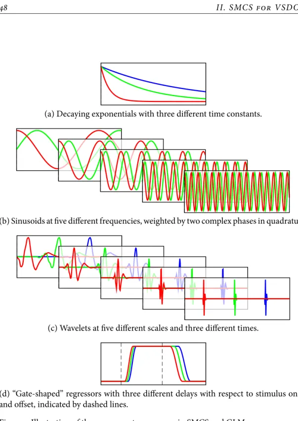
be well approximated as a linear combination of a few regressors with the right shape, or morphology. However for each component we enlarge the family of possible regres-sors: sinusoidal regressors of many different frequencies for the periodic artifacts, and an overcomplete set of wavelets for the neuronal activity. Then we look for a reconstruc-tion which is close to the observareconstruc-tion and in the same time involves as few regressors as possible. This sparsity prior enables a selection of the active regressors that is adaptive to the observation, thus allowing to separate a broader class of artifacts and neuronal
dynamics. In particular, no assumption is made about the activation time or the overall dynamic of the neuronal activity.
In order to improve further the component separation, on top of the morphology and sparsity priors on the time-course of the components, we take into account their spatial structure. To this purpose, sparsity is promoted by carefully designed spatially
structured penalizations. Periodic artifacts coefficients are penalized by a mixed ℓ1-ℓ2
-norm defined over spatial blocks of neighbouring coefficients, leading to spatially
co-herent frequency selections. In addition of a similar ℓ1-ℓ2-norm, neuronal activity
coef-ficients are also penalized by a TV semi-norm, favouring piecewise homogeneous maps of activity.
In source separation, the “blind” terminology refers to the fact that in some prob-lems, not only the sources but also their linear combination leading to the observation is unknown, and must be learn from the data; whereas in our case, the components are simply supposed to add up to form the signal. We call the resulting method spatially-structured sparse morphological component separation, abbreviated as SMCS. It is specif-ically designed to target VSDOI applications. Of course, it can be adapted to any noisy component separation problem, where the components have distinct temporal mor-phologies that can be sparsely represented in known dictionaries, and suitable spatial structures. The SMCS shares many similarities with MCA, and qualitative comparisons of those approaches are discussed.
Note finally that in the same framework, we also explore the possibility to enforce other priors than sparsity, such as bounds on amplitudes of certain components. Alto-gether, recovering the components of our model requires the solution of a convex min-imization problem of the form
find ˆx in argmin x 1 2∣∣y − Dx∣∣ 2 2+ g(Λ)(x) ,
where y is the observed signal, x are the coefficients of the different components within the linear representation D, and g is a sum of complex penalizations, depending on some parameter Λ.
Proximal Splitting Methods for Convex Optimization
The above minimization problem is convex, but high-dimensional and nondiffer-entiable, with complex relationships between the coefficients. A striking feature of the functional is, however, that the data fidelity term 12∣∣y − Dx∣∣22is differentiable, while the
penalization term g(Λ)can be decomposed as a sum of penalizations with simpler
struc-tures. Thus, the problem can be naturally recast in a more general form, as min x {F(x) def = f (x) +∑n i=1 gi(x)} , (1)
where f is smooth, and each function gi is said to be simple, in the sense that one can
compute efficiently its Moreau’s proximity operator (Moreau, 1965), defined as
proxgi(x)def = argmin ξ 1 2∣∣x − ξ∣∣ 2 + gi(ξ) .
Proximal Splitting Methods for Convex Optimization 13 This operator can be seen as an implicit version of a gradient descent, defined for pos-sibly nonsmooth convex functions.
Simple functions can be iteratively minimized through repeated applications of their
proximity operator (proximal point algorithm, Rockafellar (1976)); however, sums of
simple functions are not necessarily simple themselves. Nonetheless, a wide class of al-gorithms enables minimizing such sums, essentially by using proximity operators of each separated simple functions. They are thus called proximal splitting algorithms, and we review below their main properties and conditions of applicability.
Taxonomy of Proximal Splitting Algorithms
Certainly the most popular proximal algorithm is the forward-backward, which
ap-plies for solving(1)on any real Hilbert space H when f is differentiable with a Lipschitz
continuous gradient, and nset
= 1 with g set
= g1is simple. This scheme consists in
perform-ing alternatively a gradient descent (correspondperform-ing to an explicit step on the function f ) followed by a proximal step (corresponding to an implicit step on the function g). Such a scheme can be understood as a generalization of the projected gradient method. This algorithm, which finds its roots in numerical analysis for partial differential equa-tions, has been well-studied for solving monotone inclusion and convex optimization
problems (Bredies and Lorenz, 2008;Chen and Rockafellar, 1997;Combettes and Wajs,
2005;Gabay, 1983;Mercier, 1979;Passty, 1979;Tseng, 1991,2000). In additionBeck and Teboulle (2009)andNesterov (2013)proposed accelerated multi-step versions for
con-vex optimization, enjoying a faster convergence rate of o(1/k2) on the objective F in the
general case, where k is the iteration counter.
Other splitting methods do not require smoothness on any part of the composite functional F. The Douglas-Rachford scheme was originally developed to find the zeros
of the sum of two linear operators (Douglas and Rachford, 1956), and then two
non-linear operators inLieutaud (1969)or two maximal monotone operators inLions and
Mercier (1979), see alsoCombettes (2004);Eckstein and Bertsekas (1992). This scheme
applies to minimizing g1+g2, provided that g1and g2are simple. The backward-backward
algorithm (Acker and Prestel, 1980;Bauschke et al., 2005;Combettes, 2004;Lions, 1978;
Passty, 1979) can be used to minimize F def= g1+ g2 when the functions involved are
the indicator functions of nonempty closed convex sets, or involve Moreau envelopes.
Interestingly, if one of the functions g1or g2is a Moreau envelope and the other is
sim-ple, the backward-backward algorithm amounts to a forward-backward scheme.
Now, if L is a bounded injective linear operator, it is possible to minimize F def
=
g1○ L + g2by applying these splitting schemes on the Fenchel-Rockafellar dual problem.
It was shown that applying the Douglas-Rachford scheme leads to the alternating
direc-tion method of multipliers (ADMM) (Gabay and Mercier, 1976;Fortin and Glowinski,
1983;Gabay, 1983;Glowinski and Tallec, 1989;Eckstein and Bertsekas, 1992). For
non-necessarily injective L and g2strongly convex with a Lipschitz continuous gradient, the
forward-backward algorithm can be applied to the Fenchel-Rockafellar dual (Combettes
et al., 2010;Fadili and Peyré, 2010;Beck and Teboulle, 2014). Dealing with an arbitrary bounded linear operator L can be achieved using primal-dual methods motivated by the
classical Kuhn-Tucker theory. Starting from methods to solve saddle-point problems
such as the Arrow-Hurwicz method (Arrow et al., 1958) and its modification (Popov,
1980), or the extragradient method (Korpelevich, 1976), this problem received a lot of
attention more recently (Chen and Teboulle, 1994;Tseng, 1997;Solodov, 2004;
Briceño-Arias and Combettes, 2011;Chambolle and Pock, 2011;Monteiro and Svaiter, 2013). It is also possible to extend the Douglas-Rachford algorithm to an arbitrary
num-ber n > 2 of simple functions. Inspired by the method of partial inverses ofSpingarn
(1983, section 5), most methods rely either explicitly or implicitly on introducing
auxil-iary variables and bringing back the original problem to the case nset
= 2 in the product
space Hn. Doing so yields iterative schemes in which one performs independent parallel
proximal steps on each of the simple functions and then computes the next iterate by
es-sentially averaging the results. Variants have been proposed byCombettes and Pesquet
(2008), and byEckstein and Svaiter (2009)who describe a general projective framework
that does not reduce the problem to the case n set
= 2. These extensions however do not
apply to the forward-backward scheme, which can only handle nset
= 1.
Recently proposed methods extend existing splitting schemes to handle the sum of
any number n of composite functions of the form gi ○ Li, where each gi is simple and
each Li are bounded linear operators. Let us denote Li
∗
the adjoint operator of Li. If Li
satisfies LiLi
∗
= ν Id for any ν ∈ R∗(it is a so-called tight frame), gi○ Liis simple as soon
as giis simple and Li
∗
is easy to compute (seeProposition IV.3.7). This case thus reduces
to the previously reviewed ones. If Liis not a tight frame but(Id +Li
∗
Li) or (Id +LiLi
∗
) is easily invertible, it is again possible to reduce the problem to the previous cases by aug-menting the dimensionality by as many auxiliary variables as the number of linear
op-erator Li, each belonging to the range of Li(this is detailed in§ IV.3.1.2). Note however
that, if solved with the Douglas-Rachford algorithm on the product space, the auxiliary variables are also duplicated, which would increase significantly the dimensionality of the problem. Some dedicated parallel implementations were specifically designed for
the case where (∑iLi
∗
Li) or (∑iLiLi
∗
) is easily invertible, see for instance Eckstein
(1994);Pesquet and Pustelnik (2012). If an Li satisfy none of the above properties, it is
still possible to call on primal-dual methods, either by writing F def
= ∑igi ○ Li = g ○ l
with l(x) def
= (Li(x))i and g((xi)i) def= ∑igi(xi) (see for instance Dupé et al. (2011));
or by minimizing on the product space ˜F((xi)i)
def
= ∑i gi(Li(xi)) + ιS((xi)i) (
Briceño-Arias and Combettes, 2011), where ιSis the indicator function of the closed convex set S
defined in§ III.1.2.
Contribution: A Generalized Forward-Backward Splitting Algorithm
In spite of the wide range of already existing proximal splitting methods, none seems
satisfying to address explicitly the case where n> 1 and f is smooth but not necessarily
simple. A workaround that has been proposed previously used nested algorithms to
compute the proximity operator of∑igi within subiterations, see for instanceChaux
et al. (2009);Dupé et al. (2009);Huang et al. (2011); this leads to theoretical as well as practical difficulties to select the number of subiterations.
Splitting Structured Penalizations for Signal Processing 15 Since convex minimization problems can be recast as monotone inclusion problems, we use the more general, and somewhat more elegant, monotone operator framework. After recalling the main terminology and properties, we introduce an algorithm for
finding a zero of a sum of maximal monotone operators B+ ∑n
i=1Ai, where B is
coco-ercive. It involves the computation of B in an explicit (forward) step and the parallel
computation of the resolvents of each Aiin a subsequent implicit (backward) step. We
prove its convergence in infinite dimension, and robustness to summable errors on the computed operators in the explicit and implicit steps.
In particular, this allows efficient minimization of the sum of convex functions f +
∑n
i=1gi, where f has a Lipschitz continuous gradient and each gi is simple in the sense
that its proximity operator is easy to compute. The resulting method makes use of the regularity of f in the forward step, and the proximity operators of the simple functions are applied in parallel in the backward step.
To the best of our knowledge, it is among the first algorithms to tackle the case
where n> 1. Recently,Monteiro and Svaiter (2013)proposed an algorithm for
minimiz-ing Fdef
= f + g under linear constraints. We show in§ III.2.3how this can be adapted to
address the general problem(1), while achieving full proximal splitting and using the
gradient of f . In the process of publishing our work, we became aware that other
au-thors (Combettes and Pesquet, 2012;Condat, 2013;V˜u, 2013) have independently and
concurrently developed primal-dual algorithms to solve problems that encompass the one we consider here. These approaches and algorithms are however different from ours
in many important ways. This will be discussed in detail in§ III.2.3. We also report some
numerical experiments in§ IV.5.3, suggesting that our primal algorithm is more adapted
for imaging problems of the form(1).
This work was done in close collaboration with Jalal Fadili from the research center
GREYC (Caen, France). A significant part has been published inRaguet et al. (2013); a
notable difference with the article is a slight improvement on the relaxation constants
of the iterates, denoted ρkinAlgorithm III.1andAlgorithm III.2. On this point, we are
grateful to Yuchao Tang, Xi’an Jiaotong university, for pointing out the result ofOgura
and Yamada (2002)on the composition of two α-averaged operators, reproduced here inLemma III.1.1 (iii).
Splitting Structured Penalizations for Signal Processing
Proximal Algorithms for Inverse ProblemsAs we have seen earlier in the particular context of sparsity, numerical solutions of inverse problems often require the minimization of large scale objective functionals, taking into account both a fidelity term to the observations and regularization terms reflecting the priors one can have on the signal. Clearly, such functionals are composite by construction, hence fitting in the class of problem considered in the previous chap-ter. Within the present thesis, the most meaningful example is our SMCS variational
In many situations, this leads to the minimization of a convex functional that can be split into the sum of convex smooth and nonsmooth terms. The smooth part of the objective is often the data fidelity term, reflecting some knowledge about the forward model, i.e. the noise and the measurement or degradation operator. This is for instance the case if the operator is linear and the noise is additive and Gaussian, in which case the data fidelity is a quadratic functional. In contrast, the most successful regularizations that have been advocated are nonsmooth, what typically allows to preserve sharp and intricate structures in the recovery. In order to better model the data, composite priors can be constructed by summing several suitable regularizations, as it is the case for our
SMCS model. Moreover, while the proximity operator of the ℓ1-norm penalization is
a simple soft-thresholding (see§ IV.3.4.3), the use of complex or mixed regularization
priors justifies the splitting of nonsmooth terms into several simpler functions. In this
thesis, concrete examples are studied (see§ IV.3) and applied to our SMCS model.
Nowadays, most popular approaches for facing continuous optimization problems
rely on second-order methods, such as the ubiquitous interior-point method (Wright,
2004;Boyd and Vandenberghe, 2004). Nondifferentiable terms are taken into account by well-designed constraints; let us mention in particular that all optimization problems
considered in this thesis can be cast as conic programming (see for instanceBen-Tal and
Nemirovski (2001, section 3.3)). It is thus important here to point out the reasons why first-order methods can be preferred for many signal processing applications. Keep in
mind that those are large scale problems (usually more than 106variables), for which a
reasonable solution is not required with high-precision (because of high level of noise and uncertainty over the parameters). While second-order methods are known to give very accurate solutions in a limited number of iterations, each of those iterations re-quires the solution of linear systems growing prohibitively large with the dimension of the problem; up to the point where most machines simply cannot store the corre-sponding matrices. On the contrary, first-order methods can quickly give reasonable solutions, manipulating data whose size is of the same order of magnitude as the inputs. A last point of importance for practitioners is that second-order schemes are usually complicated to implement properly and efficiently, in comparison to the relative sim-plicity of first-order proximal algorithms.
The composite structure of convex optimization problems raised when solving in-verse problems explains the popularity of proximal splitting schemes in signal process-ing. Depending on the structure of the objective functional, one can resort to the appro-priate splitting algorithm as reviewed earlier. For instance, the forward-backward algo-rithm and its modifications are commonly used for sparse regularization of a smooth
data fidelity term, see for instance Figueiredo and Nowak (2003); Daubechies et al.
(2004);Combettes and Wajs (2005);Fadili et al. (2009);Chaux et al. (2007);Beck and Teboulle (2009);Briceño-Arias and Combettes (2009). The Douglas-Rachford and its parallelized extensions are also used in a variety of inverse problems involving only
nonsmooth functions, see for instanceCombettes and Pesquet (2007);Combettes and
Pesquet (2008);Chaux et al. (2009);Dupé et al. (2009);Dupé et al. (2011);Dupé et al. (2012);Pustelnik et al. (2011); Briceño-Arias et al. (2011). The ADMM is also applied
Risk Estimation for Parameter Selection 17
(2010). Although we make in this work only limited mention of the primal-dual schemes (Chambolle and Pock, 2011;Dupé et al., 2011), they are among the most flexible to handle
more complicated priors. The interested reader may refer toStarck et al. (2010,
chap-ter 7)andCombettes and Pesquet (2011)for extensive reviews.
Contribution: Structured Penalizations and Efficient Proximal Splitting
In view of the success of both, nondifferentiable priors for signal processing appli-cations, and their minimizations through proximal splitting algorithms, we review and extend a selective list of such priors and show how they can be split into simple func-tions.
More precisely, we propose inChapter IVa natural formalisation of structured
pe-nalizations over the Euclidean space RP, which permits to express all penalizations
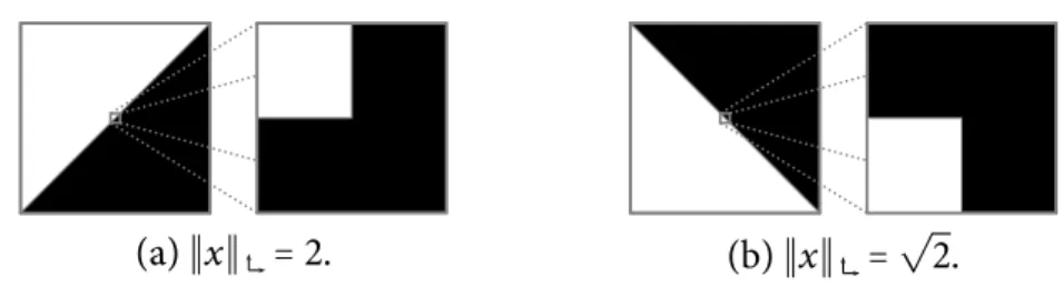
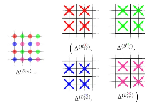
in-troduced in our SMCS model (and beyond) in a unified and concise way. We empha-size in particular structures depending on an intrinsic spatial organization of the signal, e.g. two-dimensional space for images. At this occasion, we introduce a novel discretiza-tion of the total variadiscretiza-tion semi-norm, and discuss its theoretical and computadiscretiza-tional ad-vantages over other discretization schemes.
Then, we derive the proximal formulae for each of those penalizations. Though most of these results are already known, we detail them in our specific formalization for com-prehensiveness; in addition, since they are ubiquitous in signal processing applications, we also address the general case of linear constraints and quadratic functionals. To our knowledge some results are new, such as the extensions of the proximal calculus with
the tight-frame property in § IV.3.3, and of some proximal composition properties in
§ IV.3.4.4.
The above derivations shed some light on the practical computational needs of prox-imal splitting algorithms applied to the class of problems that we consider. We iden-tify common situations where subtle implementation considerations can significantly lighten computational needs; in our opinion such matters is too often neglected in the literature, we thus expose those considerations in a setting as general as possible.
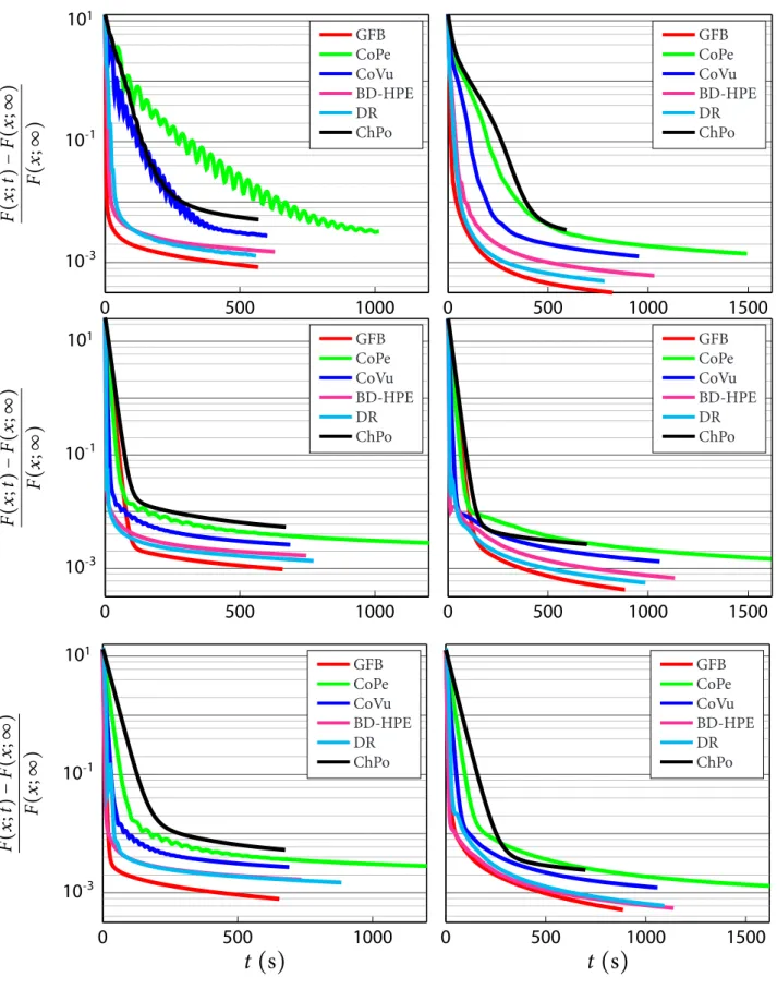
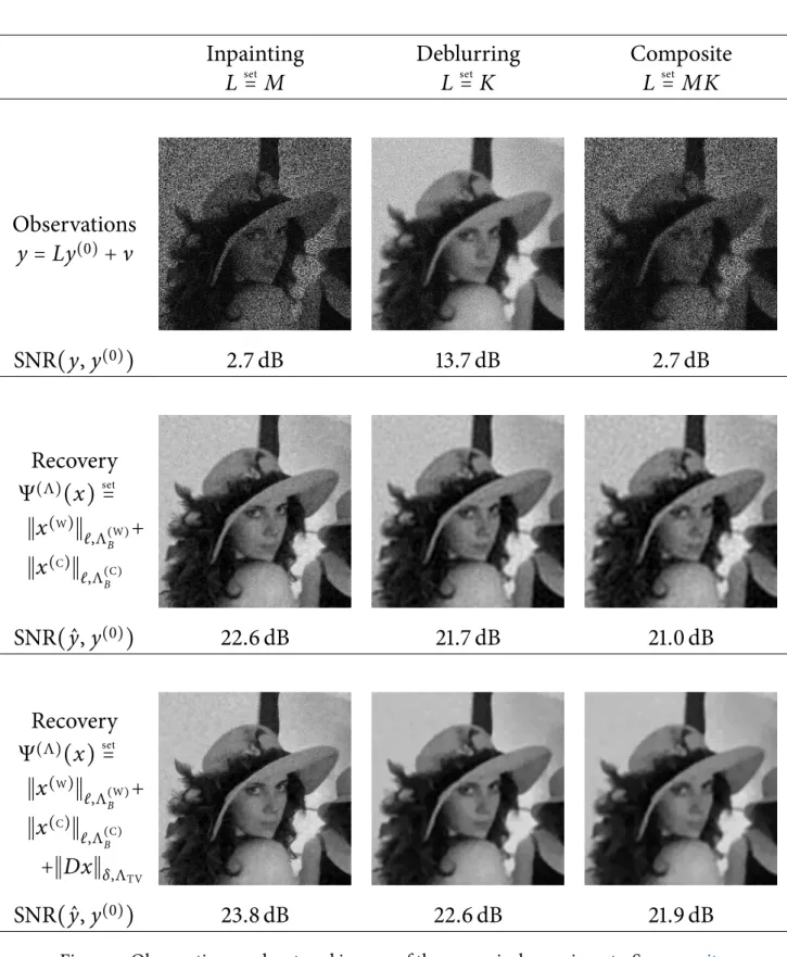
Finally, we design synthetic experiments inspired by classical inverse problems in image processing, illustrating the use of most penalizations that we defined, and en-abling comparison of various proximal splitting approaches, including our generalized forward-backward.
Risk Estimation for Parameter Selection
So far, we have seen that increasingly complex signals can be retrieved in ill-posed and noisy settings with the help of equally complex penalizations enforcing various priors. The underlying rationale is that one can replace the knowledge of the signal by the knowledge of an adapted model for it. The success of this approach is thus closely related to the quality of the model, and in particular to the accuracy of the
parame-ters defining it. In the SMCS model described in§ II, we intend to overcome the
diffi-cult noisy component separation task with a variety of different penalizations, and the problem of parameter selection becomes overwhelming.
Model Selection for Regression and Signal Reconstruction
The idea behind model selection is to view the problem as a statistical estimation, where predictions are inferred through a model fitted over a set of observations. One can then design a convenient prediction error function which evaluates the quality of an estimation given the actual observation. Typically, think at mean square errors or correlation coefficients in signal processing, or at success rate or explained variance in the context of regression and classification.
Then, following in particularEfron (2004), two main approaches for assessing the
quality of a model are cross-validation and covariance-penalties. In the cross-validation approach, the model is solved for a reduced set of observations, and one computes the prediction errors between the output of the model and the observations that has not been used. In theory, this should be computed for many different particulariza-tions of the observaparticulariza-tions to achieve statistical significance, but the generalized
cross-validation introduced byGolub et al. (1979)does not require so many computations of
the model. The advantage of the cross-validation approach is that it usually does not as-sume any generative model on the data, and is in that sense nonparametric. In contrast, the covariance-penalties approach involves in some way an estimation of the covariance between the estimations and the data, which requires assumptions about their statistical distribution. In the context of signal processing, this often reduces to the knowledge of
the noise statistics, and can be estimated in many cases (see in particular§ V.1.3).
For that reason, covariance-penalties approaches are preferred for the targeted
ap-plications (seeLi (1985);Efron (2004)); one of the most popular being Stein’s unbiased
risk estimate (SURE), because it applies to a wide range of nonlinear models, and is es-pecially well-designed for Gaussian noise. In brief, Stein’s lemma states that, provided weak differentiability conditions of the estimation function (coined estimator), the above covariance can be estimated on the derivatives of that function. Hence, the risk of the estimation, which is the expectation of the squared error between the estimate and the original signal, taken according to the noise statistics, can be unbiasedly estimated. By computing it for different values of a parameter tuning the model, one can select the parameter minimizing the SURE.
Parameter selection with the SURE specifically for signal processing goes back at
least toDonoho and Johnstone (1995), where its expression is derived for the ℓ1-norm
denoising estimator and used for scaling the penalization. Extensions have been sub-sequently developed to other penalizations such as the ones we consider in this work, (Chaux et al., 2005;Zou et al., 2007;Chaux et al., 2008;Yu et al., 2008;Chesneau et al., 2010; Solo and Ulfarsson, 2010; Dossal et al., 2013) and beyond (Vaiter et al., 2014). Successful applications have been reported for numerous signal denoising tasks (see for
instanceBlu and Luisier (2007);Van De Ville and Kocher (2009);Luisier et al. (2010a);
Deledalle et al. (2012a);Duval et al. (2011);Van De Ville and Kocher (2011);Ramani et al. (2012a)). In the same time, theoretical developments ofEldar (2009)enabled the
adap-tion of the SURE to non-Gaussian noise (Luisier et al., 2010b), and to inverse problems
beyond denoising (Pesquet et al., 2009). Let us finally mention some numerical
meth-ods which do not require the computation of the derivatives of the estimator explicitly,
A Full Component Separation Method for VSDOI 19
2014), or, in the case of estimators defined by iterative algorithms, by recursive
deriva-tions (Vonesh et al., 2008;Giryes et al., 2011;Ramani et al., 2012b).
Contribution: Risk Estimation for Proximal Denoising
InChapter V, we first redefine rigorously the terms and conditions of the SURE for denoising problems with arbitrary Gaussian noise. Then, in the continuity of the previous chapters, we emphasize the fact that any proximity operator can be seen as a denoising estimator, and satisfies the regularity conditions for estimating its risk with the SURE. We give the SURE expressions of the proximity operators of the penalizations defined previously, and study the more involved case of a denoising estimator penalized
by reweighted ℓ1,2-norm, inspired by the reweighted ℓ1-norm ofCandès et al. (2008).
We then turn to denoising estimators that cannot be reduced to proximity opera-tors of simple functionals, establishing in particular a proper chain rule for Lipschitzian functions in arbitrary dimension, which is actually a theoretical prerequisite of the re-cursive derivation method mentioned above. After describing the practical computa-tional limitations of their use for our purpose, we propose a series of heuristics allowing fast and efficient approximations.
Finally, we exemplify the use of the SURE for parameter estimation in an image denoising setting, and test empirically our heuristics.
A Full Component Separation Method
for Voltage-Sensitive Dye Optical Imaging
With all the mathematical and computational tools developed in this thesis, it is pos-sible to apply our spatially structured sparse morphological model to voltage-sensitive
dye optical imaging data. InChapter VI, we expose briefly the rationale that allows us
to adapt to component separation problems parameter selection methods originally de-signed for simple denoising problems. This adaptation requires notably successive ap-proximations of the different components involved in the problem and estimations of the noise statistics. We show that under convenient assumptions, this is actually possible for VSDOI data; in particular, some first approximations involve processing of blank ac-quisitions, i.e. acquisitions recorded without specific stimulus presented to the animal, where we assume that only few neuronal activity is present.
Note that the full method, from parameter selection to the resolution of the varia-tional problems, is now decomposed into several interrelated steps. Moreover, at each of those steps, some practical choices remain to be taken. Everything is explained in
details withinChapter VI, and summarized onTable VI.1.
Altogether, we implement the full methods and perform the first experiments for
evaluating it. InChapter VII, we first investigate the contributions within the highest
frequencies of VSDOI recording, validating in particular the model of the noise
pro-posed in§ II.2.1. Then, we run numerical experiments over synthetic data, mimicking
real VSDOI data, which allows us to work in a controlled environment and to know the actual targeted components. On such an “oracle” setting, we attest relatively good
per-formances of our method, and we evaluate its pros and cons in comparison to a GLM method. Third, we test the possibility of retrieving actual functional signals, on the well-studied orientation selectivity of the cat’s primary visual cortex, thanks to data provided by Cyril Monier. Without delving into further functional details, we make use at this
oc-casion of preliminary results of the extensive study inYavuz (2012). At last, we explore
visually the output of our method on data presenting propagating neuronal activity in the mouse’s somatosensory cortex, provided by Isabelle Ferezou. Since such propaga-tions can be evoked by specific stimuli but also spontaneous, we show in particular the ability of our method to retrieve neuronal activity in paradigm-free conditions.
Thanks to those preliminary sets of experiments, it is already possible to discuss the validity of the method, especially concerning the assumptions that we made over
the VSDOI signal inChapters IandII. In addition, we discuss the practical conditions
which render difficult the use of the current version of the full method by practitioners.
∗
∗ ∗
I
Voltage-Sensitive Dye Optical Imaging
Ways and Customs
In this chapter, we describe the optical imaging technique based on voltage-sensitive dye for monitoring the cortical neuronal activity at population level. First, we briefly de-scribe its principles and capabilities, pointing out the interest of improving this acquisi-tion modality for the neuroscientific community. Doing so, we introduce the motivaacquisi-tion and problematic that are behind the whole work of signal processing presented in this thesis.
We describe also the main causes of limitations encountered by experimentalists and analysts, and the inevitable need for signal processing when dealing with voltage-sensitive dye optical imaging. Finally, a critical review of approaches found in the liter-ature is given and discussed as the starting point of our own reflection.
C ontents
1 Monitoring Cortical Activity with VSDOI. . . . 22
1.1 Electrophysiological Background. . . 22 1.2 The VSDOI Modality. . . 24 1.3 The Targeted Signal. . . 26
2 The Challenge of VSDOI in vivo . . . . 28
2.1 What Are We Recording? . . . 28 2.2 Sources of Noise and Artifacts . . . 29 2.3 Modeling the Signal . . . 30
3 VSDOI Denoising: Previous Approaches . . . . 30
3.1 Blank Subtraction. . . 31 3.2 Baseline Fluorescence, Gain and Bleaching . . . 33 3.3 Heartbeat Triggered Averaged . . . 34 3.4 Automatic Component Separation Methods . . . 34 3.5 General Linear Model . . . 35 3.6 Towards Better Denoising Methods . . . 36
Appendix . . . . 38
A Subtraction Approximates Division . . . 38
References . . . . 38
1
Monitoring Cortical Activity with VSDOI
1.1
Electrophysiological Background
It is common to consider that modern neuroscience starts with the work of Santiago Ramón y Cajal and Camillo Golgi at the end of the nineteenth century, leading to the neuron theory, mostly formulated by Heinrich Wilhelm Gottfried von Waldeyer-Hartz. To date, it is still assumed that most if not all information in the brain is encoded within electrical activity of the nerve cells, the neurons. In brief, the neurons are cells covered by ion gates which control the relative concentrations of certain ions between the in-tracellular and exin-tracellular media, governing in turns the electrical potential between each side of the cellular membrane. Neurons are interconnected by their neurites, which are projections of their cell body. Among them, the axon sends information to other neurons, and the dendrites collect information from other neurons. The neurons are
1. Monitoring Cortical Activity with VSDOI 23 considered as the elementary processing units, but even the simplest brain functions emerge from the activity of millions of such neurons, interconnected into hierarchical spatial structures, and following specific temporal dynamics.
In order to understand the brain from a computational point of view, it seems nec-essary to have access to the operating modes of single neurons, as well as their relation-ship one to the other within each organization level. To this end, the most direct way of recording electrical activity is to put electrodes inside the brain tissue. This can be done either in vitro (in specific preparations, usually slices of animal brain), or in vivo in living animals. Intracellular recordings have the highest accuracy and informs the best on how single neurons work. This allowed Alan Lloyd Hodgkin and Andrew Fielding Huxley to explain the spiking nature of the neuronal activity. The electrical potential of a neuron fluctuates along time because of the activity of other neurons; whenever this potential reaches a critical value, cellular mechanisms within the neuron trigger a fast additional increase of potential of huge amplitude that lasts only for a very short period of time, and propagates along its axon. Those events are called action potentials, and take place within the temporal order of the millisecond. In the same context, extracellular record-ings are often easier to perform, and depending on the electrode size can probe the activity of one or several neurons. In the last case, it is in general difficult to isolate the contribution of each neuron, but it already enables to study the relationships between them.
The biggest advantage of using electrodes is that they have high spatial and tem-poral resolutions, i.e. they can capture every events that take place along time, at mi-croscopic scales. Moreover, it enables recordings wherever it is physically possible to introduce electrodes without damaging the surrounding tissues. Now, though it is pos-sible to record simultaneously from several electrodes, this raises technical difficulties (Lampl et al., 1999) and it is obvious that networks of thousands of neurons cannot be observed by those techniques. In an other approach, electroencephalography consists in many electrodes put all over the surface of the head. Those can be recorded for days, and even on human brain since it is noninvasive. However, the resulting spatial resolution is very crude, and only the synchronous activity of thousands of neurons situated at the surface of the brain can be detected that way.
Currently, no other technique gives such direct access to the electrical activity of the neurons. Nevertheless, the brain functions can be investigated indirectly through physi-ological phenomena that relate to them. For instance, intrinsic physiphysi-ological changes oc-cur locally whenever significant neuronal activity is triggered, such as increase in blood volume and changes in hemoglobin oxymetry. Then, labelling techniques can be used to identify which brain regions are recruited during specific tasks. They usually involve the injection of specific tracers in the blood of the animal under investigation. Those tracers are usually molecules that can be later on easily detected, either post mortem for sim-ple dyes, or in vivo thanks to radioactive or magnetic properties. High concentration of tracers indicates regions of high activity. The most notable example is the positron emission tomography which uses radioactive tracers and can be used in human subjects. Labelling methods can screen the whole brain, but like electroencephalography pro-vides only coarse, macroscopic functional information. Worst, each image usually takes
minutes to acquire, so that dynamical aspects cannot be captured. The development of functional magnetic resonance imaging (fMRI) enhances drastically macroscopic obser-vations of the brain functions. The most common method is to detect the intrinsic signal by exploiting the difference of magnetization of the blood according to its oxygen con-centration. Currently, the spatial resolution goes up to the order of the millimeter, and the temporal resolution reaches the order of the second.
Intrinsic signal can also be observed with intrinsic optical imaging, by shedding near infrared light on the surface of the cortex, and recording over time the changes in re-flectance induced by the intrinsic changes. Since the acquisition principle is simpler
than for fMRI, the spatial resolution reaches nowadays the tenth of a millimeter (Zepeda
et al., 2004). Only a limited part on the surface of the cortex can be studied this way, but at this level of precision it becomes possible to distinguish specialized group of neu-rons that acts as functional units, like orientation columns in mammalian primary visual
cortices (Rao et al., 1997). Still, temporal resolution cannot be improved because of the
time scale of the intrinsic changes, which happens seconds after an actual, significant neuronal activity.
The great interest of the voltage-sensitive dye optical imaging (VSDOI), which is the measurement modality at the heart of this thesis and is described in more details in the next section, is that it can, in theory, combine the mesoscopic spatial scale of optical imaging with the real-time temporal resolution of direct electrophysiological measure-ments.
1.2
The VSDOI Modality
1.2.1 Principles.Sensitivity to membrane potential of some fluorescent dyes is known for long (at
least back toCohen et al. (1974)), and its use for monitoring neuronal activity has been
considered ever since. Starting with recordings of action potentials in individual
neu-rons (Davila et al., 1973;Salzberg et al., 1973), the technique got continuously improved
along time, and is now a privileged modality for monitoring cortical activity
simultane-ously at several locations with both high spatial and temporal resolution (Grinvald and
Hildesheim, 2004).
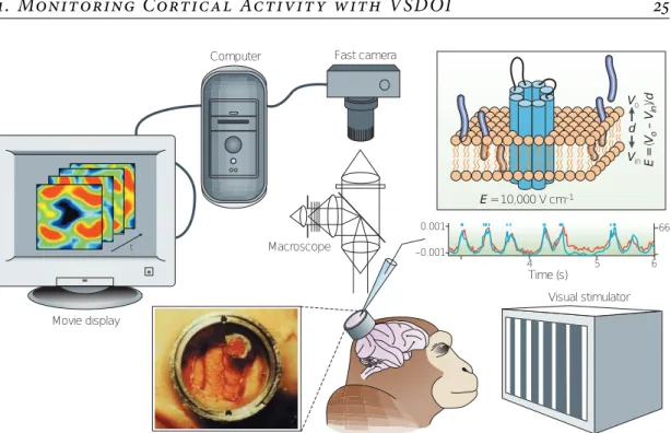
To perform VSDOI one stains the neuronal tissue with voltage-sensitive dye, which are fluorescent molecules, also called fluorophores. Some of those bind to neurone mem-branes. Each fluorophore, when illuminated with the correct exciting wavelength, emits light in a different wavelength in return. The fluorophores that are bound to a neurone membrane happen to emit differently according to the electrical potential at the mem-brane. Thus, filming the emitted fluorescence provides access to the variations of the
potential of those membranes along time. The whole process is schematized inFigure 1,
see for instanceGrinvald et al. (1999)orFrostig (2009)for detailed practical
1. Monitoring Cortical Activity with VSDOI 25 0.001 –0.001 66 4 5 6 Time (s) Visual stimulator Movie display E = 10,000 V cm–1 Vin Vo d E = ( Vo – Vin )/ d Fast camera Macroscope Computer t
Figure 1: Schematic view of a VSDOI set-up. Reproduced fromGrinvald and Hildesheim
(2004).
1.2.2 Limitations.
Because the changes in fluorescence follow closely a change in membrane potential, both in time (order of the microsecond) and in space (at molecular scale), the resolution of VSDOI is in theory only limited by two main factors: the quantum nature of photon emissions, and the precision of the optical recording device.
Recorded fluorescence intensity corresponds to the count of the number of pho-tons reaching the detector during a certain time laps. At a given intensity, the number of emitted photons during a given duration is best modeled by a Poisson distribution (Foschini et al., 1975), for which the variance increases proportionally to the mean level. Hence, the expected quality of a fluorescence measurement, quantified by the ratio be-tween the mean number of emitted photons and its standard deviation, is proportional to the square root of the mean number of photons. As a consequence, it is important to maximize the mean number of photons recorded at each measurement. This is in turn proportional to three main factors: the number of fluorophores within the focus of the detector, the duration of each measurement, and the intensity of the exciting light. In any experimental set-up, a compromise must be found between those three factors, in accordance with the instrumental and material conditions.
On the one hand, the quantity of fluorophores reporting potential changes is limited by the total area of neuronal membrane under investigation, and by the physical access to those membranes. Moreover, the quantity of fluorophore introduced in the medium must also be limited in order to avoid pharmacological effects, i.e. perturbations of the functioning of the neurons due to the presence of the fluorophores. Similarly, the in-tensity and the duration of the exposure of the exciting light is limited by photodynamic
damage that can occur to the medium. See for instanceGrinvald et al. (1999)andPeterka et al. (2011)for more details on those practical limitations.
On the other hand, optical precision is limited by light scattering and focal preci-sion, while the quantity of data recorded during a certain amount of time is limited by acquisition and data-storage speed. Horizontal spatial resolution (parallel to the cortical surface and orthogonal to the optical axis) goes below a tenth of a micron when using
confocal (Holthoff et al., 2010) or two-photon (Acker et al., 2011) microscopy. This
ac-tually allows to discriminate between neuron compartments. Unfortunately, only two-photon techniques allows such precision in the vertical axis. For all other recording techniques, the focal plan is much thicker. This can be limited in vitro by reducing the thickness of the sample itself (thin brain slices), but in vivo, contributions of several cortical layers might be mixed in the signal, depending on the dye distribution along the depth of the cortex. Concerning the spatial extent of the field of view, most
com-mercial devices available nowadays exceed 1000× 1000 pixels, and temporal resolution
goes up to 10 kHz, allowing to capture every events of an action potential (Tominaga
and Tominaga, 2013).
The final compromise between spatial and temporal resolution, data quantity, and recording quality depends on the phenomena under investigation and on the exper-imental conditions. In particular, in vitro experiments allows more flexibility than in vivo, but does not give access to the same information. In all the present work we are mostly interested in in vivo recordings, at population level, with spatial resolution be-tween 10 and 100 µm, sampling frequency bebe-tween 100 Hz and 1 kHz, and spatial extent
no more than 100× 100 pixels.
1.3
The Targeted Signal
Before diving into the technical aspects of VSDOI signal processing, let us describe the phenomena one would like to investigate thanks to the VSDOI modality. Those con-siderations are useful in order to understand the motivation and ambition that lies be-hind the work developed in this manuscript.
1.3.1 The Cortical Phenomena Under Investigation
The use of VSDOI at single cells level is justified when direct intracellular recording is rendered impossible, often because it is too invasive or because the targeted site is too small for the insertion of an electrode. However, the advantage of the VSDOI modality which is the most interesting to us is its ability to record in real-time the activity of en-tire networks comprising thousands of neurons. At the population level, VSDOI is more sensitive to subthreshold potential variations of many synchronous neurons than to
in-dividual spiking activity (Chemla and Chavane, 2010a). Although it does not reveal the
action potentials, such mesoscopic information is useful to understand the mechanisms of integration of individual neurons activity within local networks. In particular, spa-tiotemporal dynamics of functional structures, population encoding of sensory stimuli,
1. Monitoring Cortical Activity with VSDOI 27
and Hildesheim (2004)andChemla and Chavane (2010a)for more details on the cor-tical mechanisms best revealed by VSDOI.
1.3.2 The Question of the Ongoing Activity
When studying functional organization of the cortex, the usual approach is to ana-lyze the activity evoked in vivo by certain stimuli. However, it has been observed that the variability of the neuronal response to several repetitions of the same stimulus is
some-times as significant as the response itself; seeArieli et al. (1995)and references therein.
Moreover, even in the absence of specific stimulus, neurons exhibit spontaneous activ-ity that is often highly structured in space and time, at both at the single cell level and at the population level. This spontaneous or on-going activity can be observed with any recording modality, and presents a wide variety of dynamics, usually highly dependent to the conscious state of the subject (anesthetized or awake).
Many important questions arise about the on-going activity. Neither its origin and mechanisms, nor its relationship to the activity evoked by a specific stimulus and its role in perceptual attention is yet well understood. Experiments with VSDOI could provide precious information, but let us emphasize here that on-going activity is also an obstacle for VSDOI recordings at population level. As described in the next section, VSDOI ac-quisitions are corrupted by many nonneuronal artifacts, so that up to now information is extracted by averaging over repetitions, or using ad-hoc processing methods retriev-ing the evoked, reproducible signal and discardretriev-ing the variability. Although VSDOI has
already been used in studies of ongoing dynamics (see againArieli et al. (1995), orArieli
et al. (1996)), precaution must be taken for their interpretation. This underlines the need for new processing methods that would capture all the variability at the single acquisi-tion (also dubbed trial) level.
On a VSDOI signal processing point of view, it is important to distinguish several temporal and spatial scales of ongoing dynamics. At the lowest frequency scale, sponta-neous organization of cortical assemblies presents up and down states, that are respec-tively depolarized and hyperpolarized temporary states, resulting respecrespec-tively in higher and lower activity levels for durations in the order of the second. Such slow fluctua-tions are usually associated with high level of synchrony, involving entire networks at
the spatial scale of the millimeter, see for instanceLampl et al. (1999); Petersen et al.
(2003). Then, faster spontaneous events that are often reported concern propagating waves of activity running across neuronal networks, especially in the cortex. Such events are highly structured, and usually closely resemble events that can be evoked by specific stimuli. They are however very diverse, with many different propagation velocities and spatial extents, with frequency scales in order of magnitude from 1 up to 100 Hz, see for
instance the review ofMuller and Destexhe (2012). Finally, individual neurons within
networks always exhibit fluctuations of activity, both in term of spiking activity and of subthreshold potential variations, due to a wide variety of sources and often considered
as random noise (Destexhe and Rudolph-Lilith, 2012). Notably, these fluctuations might
have temporal components above 100 Hz and show little correlation from one neuron to another.
or might not, have actual biological relevance. However, they seem to relate to distinct phenomena and, more importantly, their respective influences on VSDOI acquisitions are as significant as they are different.
2
The Challenge of VSDOI in vivo
In spite of the constant enhancement of the VSDOI technique along several decades, in vivo recording remains a technical challenge, due to a wide variety of artifacts and noise that corrupt the signal, and that can also differ greatly according to the experi-mental conditions.
2.1
From Fluorescence to Neuronal Activity:
What Are We Recording?
As introduced in§ 1.2.1, the fluorophores bound to a neuronal membrane fluoresce
differently according to the electrical potential at the membrane. This knowledge, how-ever, is not sufficient to deduce changes in neurons membrane potential. First of all, hundreds to thousands of neurons contribute to each single pixel of the recorded ac-quisition and it is impossible to differentiate between contributions of axonal or den-dritic activity, of inhibitory or excitatory neurons, or even of some nonneuronal cells
(glia, etc.). The different contributions have been studied in particular byChemla and
Chavane (2010b). In general, the best information available is the variation of membrane potential averaged over multiple compartments of multiple cells, integrated over several cortical layers. Moreover the interpretation of this variation of membrane potential is delicate because one does not know the baseline activity, the reference value to which the variation should be computed.
Now, how does one link the VSDOI acquisition to this average potential variation? The mechanism linking variations in membrane potential to variations in fluorescence
has already been investigated (Peterka et al., 2011) and the relationship between those
variations is supposed to be linear. But what is the gain of this linear relationship? For a given spatial position and at a given instant (a pixel of a frame in the acquisition), it should depend on the quantity of fluorophores bound to the membrane and to the illu-mination intensity. Here again one often assumes linear relationship between intensity
of fluorescence and fluorophore concentration, see for instanceTanke et al. (1982)in
the context of microscopy. Also, keep in mind that only fluorophores bound to a neu-ronal membrane contribute to the desired signal, so that the area of stained membrane should be taken into account as well. Unfortunately one does not have access to all these information.
Moreover, VSDOI records the absolute fluorescence intensity (i.e. the number of photons detected during the frame duration at each pixel). In order to get variations of fluorescence, one needs another baseline value, the baseline fluorescence, that is to say the fluorescence intensity that would be recorded independently from any neuronal ac-tivity (and from other existing biophysical sources of variations). Baseline acac-tivity and