Stochastic Volatility for L¶evy Processes
¤
Peter Carr
Banc of America Securities
H
elyette Geman
University of Paris IX Dauphine and ESSEC
Dilip B. Madan
Robert H. Smith School of Business
University of Maryland
Marc Yor
Laboratoire de probabilit
es et Modeles al¶eatoires
Universit¶e Pierre et Marie Curie
4, Place Jussieu F 75252 Paris Cedex
April 16 2001
Abstract
Three processes re°ecting persistence of volatility are formulated by evaluating three L¶evy processes at a time change given by the integral of a square root process. A positive stock price process is then obtained by exponentiating and mean correcting these processes, or alternatively by stochastically exponentiating the processes. The characteristic functions for the log price can be used to yield option prices via the fast Fourier transform. Our empirical results on index options and single name options suggest advantages to employing higher dimensional L¶evy systems for index options and lower dimensional structures for single names. In general, mean corrected exponentiation performs better than employing the stochastic exponential. Martingale laws for the mean corrected exponential are also studied and two new concepts termed L¶evy and martingale marginals are introduced.
¤We would like to thank George Panayotov for assistance with the computations reported in this
paper. Dilip Madan would like to thank Ajay Khanna for important discussions and perspectives on the problems studied here. Errors are our own responsibility.
Sto chastic Volatility for L¶e vy Pro ces se s
April 16 2001
Abstract
Three processes re°ecting persistence of volatility are formulated by evaluating three L¶evy processes at a time change given by the integral of a square root process. A positive stock price process is then obtained by exponentiating and mean correcting these processes, or alternatively by stochastically exponentiating the processes. The characteristic functions for the log price can be used to yield option prices via the fast Fourier transform. Our empirical results on index options and single name options suggest advantages to employing higher dimensional L¶evy systems for index options and lower dimensional structures for single names. In general, mean corrected exponentiation performs better than employing the stochastic exponential. Martingale laws for the mean corrected exponential are also studied and two new concepts termed L¶evy and martingale marginals are introduced.
1
Introduction
It has been clear that the standard option pricing model of Black-Scholes [8] and Merton [30] has been inconsistent with options data for at least a decade. Despite this result, no other model comes close to the popularity of the Black Merton Scholes (BMS) model in both theory and practice A partial explanation lies in the simplicity of the BMS model. Models which produce superior empirical performance almost always require more parameters, and consequently are usually signi¯cantly slower in terms of both calibration and computation.
The empirical performance of a potential successor to BMS is usually measured in terms of hedging and/or pricing performance. This performance can be analyzed in
terms of at least four ubiquitous inputs, which are calendar time, the underlying's price, the option's term, and the options's strike. While capturing the e®ect of variation in these four inputs should improve the overall performance, capturing the e®ect of variation in the ¯rst pair is particularly important for reducing risk, while capturing the variation with respect to the latter pair is critical for reducing pricing error.
To improve on the pricing and hedging performance of the BMS model, the majority of the research has been directed towards modifying the continuous time stochastic process followed by the underlying asset. In particular, asset returns have been modeled as di®usions with stochastic volatility (eg. Hull and White[23] or Heston [22]), as jump-di®usions (eg. Merton [31] or Kou[25] ), or both (eg. Bates [6] [7] or Du±e, Pan, and Singleton [14]). Empirical work on these models has generally supported the need for both stochastic volatility and jumps. Stochastic volatility appears to be needed to explain the variation in strike at longer terms, while jumps are needed to explain the variation in strike at shorter terms. Furthermore, jumps and the inability to trade continuously are usually the favored explanations for the existence of substantial hedging errors, whose persistence has been documented repeatedly.
On the theoretical side, arguments have been proposed by Geman, Madan, and Yor [20] which suggest that price processes for ¯nancial assets must have a jump component, while they need not have a di®usion component. Their argument rests on recognizing that all price processes of interest may be regarded as Brownian motion subordinated to a random clock. This clock may be regarded as a cumulative measure of economic activity, as conjectured by Clark [12], and as estimated by An¶e and Geman [1]. As time must be increasing, the random clock can be modelled as a pure jump increasing pro-cess, or alternatively as a time integral of a positive di®usion propro-cess, and thus devoid of a continuous martingale component. If jumps are suppressed, then the clock is locally deterministic, which they rule out a priori. Thus, the required jumps in the clock in-duce jumps in the price process, while no argument similarly requires that prices have a di®usion component.
The explanation usually given for the use of jump di®usion models is that jumps are needed to capture the large moves that occasionally occur, while di®usions are needed to capture the small moves which occur much more frequently. However, since at least the pioneering work of Mandelbrot [26] on stable processes, it has been recognized that many pure jump models are able to capture both rare large moves and frequent small moves. Motivated by the possibility that price processes could be pure jump, several authors have focussed attention on pure jump models in the L¶evy class. Technically, these processes can capture frequent small moves through the use of a L¶evy density whose spatial integral is in¯nite
There are at least three examples of such pure jump in¯nite activity L¶evy processes. First, we have the normal inverse Gaussian (NIG) model of Barndor®-Nielsen [4], and its generalization to the generalized hyperbolic class by Eberlein, Keller, and Prause [15]. Second, we have the symmetric variance gamma (VG) model studied by Madan and Seneta [29] and its asymmetric extension studied by Madan and Milne [28], Madan, Carr, and Chang [27]. Finally, we have the model developed by Carr, Geman, Madan, and Yor (CGMY) [10], which further generalizes the VG model. CGMY study the empirical adequacy of the VG and CGMY models in explaining equity option prices across the strike range. They ¯nd that these models can explain the so-called volatility smile, and that the empirical performance of these models is typically not improved by adding a di®usion component for returns. These results raise the disturbing question as to whether di®usion components are needed at all when modeling asset returns.
The empirical success of pure jump L¶evy processes is not maintained when one con-siders the variation of option prices across maturity. It has been observed in Konikov and
Madan [24] that these homogeneous L¶evy processes impose strict conditions on the term structure of the risk-neutral variance, skewness, and kurtosis. Speci¯cally, the variance rate is constant over the term, skewness is inversely proportional to the square root of the term, while kurtosis is inversely proportional to the term. In contrast, the data sug-gests that these risk-neutral moments are often rising with term. Economically, the usual supposition that investor uncertainty is increasing with the term suggests that return distributions should spread out as the holding period is increased. On the other hand, risk premia in markets are likely to display mean reversion, which would impact the term structure of skewness and kurtosis implicit in the risk-neutral distribution. Collectively, these considerations suggest that it may be desirable to incorporate a richer behavior across maturity than is implied by homogeneous L¶evy processes.
In a parallel development in the literature, it has been observed by several authors such as Engle [16], Bates [6], [7], Heston [22], Duan [13], and Barndor®-Nielsen and Shephard [5], that volatilities estimated from the time series are usually clustered, which is commonly referred to as volatility persistence. This persistence is inconsistent with homogeneous L¶evy processes, and possibly explains the failure of such processes to explain option prices across the maturity dimension.
For these reasons, the objective of this paper is to extend the otherwise fairly successful L¶evy process models cited above by incorporating stochastic and mean-reverting volatil-ities. We take three homogeneous L¶evy processes, viz the N IG; V G; and the CGMY models, and generate the desired volatility properties by subordinating them to the time integral of a Cox, Ingersoll, and Ross [11] (CIR) process. The randomness of the CIR process induces stochastic volatility, while the mean reversion in this process induces volatility clustering. We term the resulting processes N IGSV; V GSV; and CGM Y SV in recognition of their synthesis with stochastic volatility. These processes are tractable in that analytical expressions can be derived for their characteristic functions. On em-ploying their exponentials to describe stock prices, European options can be priced via Fourier methods as described in Bakshi and Madan [3] and Du±e, Pan and Singleton [14]. In particular, the current paper applies the fast Fourier transform (FFT) method, which is developed in Carr and Madan [9].
The three new processes collectively provide us with a °exible family of option pricing models, capable of being calibrated to market option prices varying across both the strike and maturity dimensions. The calibrated process may then be used for pricing standard options not included in the calibration or for pricing exotic options. These processes can also be used in a simulation to evaluate the quality of hedging strategies, by for example pricing claims whose payo®s are functions (eg. squares) of the cumulative hedging error. These new stochastic processes can thereby be used to enhance our structural understanding of risk management issues. With the resulting models, one may assess the impact on market values of changes in reasonably intuitive parameters such as the speed of adjustment, the level of long run volatility, and the variance of volatility. Thus, the parameters of the models synthesize the information content of option prices in a concise manner, and open the door to interesting investigations into the economic determinants of asset pricing as inferred from an analysis of derivative markets.
In constructing risk-neutral price processes from the N IGSV; V GSV; and CGM Y SV processes, two approaches are followed. The approaches di®er in terms of the ¯ltration in which the martingale condition is based on. The ¯rst approach assumes that investors can only condition trades on the level of the stock price, while the second approach assumes that trades can also be conditioned on the level of the L¶evy process and the time on the new clock. Thus, the ¯rst approach prohibits arbitrages based only on the stock price, while the second approach further precludes arbitrages based on the level of the driving L¶evy process and the new clock. The reason that the two approaches were tried is that
one can argue that the stock price is far more observable in practice than either of the variables used to model the stock price process.
To operationalize the ¯rst approach, we construct the risk-neutral distribution for the stock price at each future time as the exponential of N IGSV; V GSV; and CGM Y SV pro-cesses, normalized to re°ect the initial term structure of forward prices. This procedure ensures that spot-forward arbitrage is not possible. We also exclude arbitrages involving calendar spreads of options as these also require knowledge of just the stock price (at the earlier maturity) The class of models generated by excluding price-based arbitrages are termed NIGSA; V GSA; and CGM Y SA respectively. The second approach is opera-tionalized by compensating the pure jump processes NIGSV; V GSV; and CGY M SV to form martingales. These martingales are then stochastically exponentiated to yield mar-tingale candidates (in the enlarged ¯ltration of the L¶evy process and the integrated CIR time change) for forward prices. This class of models is termed N IGSAM; V GSAM; and CGMY SAM respectively. Characteristic functions for the log of the stock price are formulated analytically in all 6 cases. These characteristic functions are used to generate model option prices numerically, which are then compared with the data.
We note that the N IGSAM; V GSAM;and CGMY SAM models are martingales with respect to the enlarged ¯ltration, which includes knowledge of the driving L¶evy process and knowldege of the subordinator given by the time-integrated CIR process. To the extent that these two processes can not be separately ascertained from a time series of prices, serious issues arise as to the practical relevance of the associated martingale condition. Working with purely discontinuous price processes, Geman, Madan, and Yor [21] provide a precise formulation of conditions under which the two processes can be determined from the time series of underlying asset prices. Even if the two processes can be determined from a time series, it is unlikely that the rich dynamics of the option price matrix can be adequately captured by a martingale which re°ects movements in only two processes. Hence, if the market is precluding arbitrage based on a richer ¯ltration than the one generated by the two processes, one is again forced to confront the practical relevance of martingale conditions which are based on ¯ltrations that are essentially unobservable. The models NIGSA; V GSA; and CGM Y SA take a more conservative approach than the martingale models N IGSAM; V GSAM; and CGM Y SAM . Relying only on the abil-ity to observe stock prices, these models generate stock price processes whose risk-neutral expectation is consistent with the initial term structure of forward prices, but which do not require that these forward prices be martingales with respect to the ¯ltration gen-erated by the Levy process and the subordinator. We ¯nd that these more conservative models consistently provide substantially superior empirical performance over the models which prohibit arbitrage based on the richer and perhaps unobservable ¯ltration. Given these results, we take up a deeper study of the properties of these more conservative models . In this regard, we introduce two important new concepts, which we term the martingale marginal property and the L¶evy marginal property . We de¯ne a process as having the martingale marginal property if it has the same marginal distributions as some martingale process. We further de¯ne a process as having the L¶evy marginal property, if it has the martingale marginal property and if the martingale is derived from normal-izing the exponential of a time inhomogeneous L¶evy process. We show ¯rst that if the CIR process is started at zero; then our conservative processes have this L¶evy marginal property. When the starting value is not zero; we conjecture that these processes have the martingale marginal properties.1 Although these questions may be investigated com-putationally by constructing L¶evy densities associated with the characteristic functions of the processes, we pursue a richer understanding of the possibilities by structurally
1At this writing, necessary conditions for this property in some parametric special cases have been
reconstructing the one dimensional distributions in alternative ways. This leads to an attractive representation in the form of an inhomogeneous L¶evy process perturbed by a process for conditional abnormal returns that are unconditionally absent and eventually zero. Whether trading strategies may be formulated to exploit this information is an open question.
We report the results of estimating all six models using S&P 500 option closing prices for the second Wednesday of each month of the year 2000. For other underliers, we report on just the dominating three models N IGSA; V GSA; and CGM Y SA: In the interests of brevity, we provide here a sample of quarterly results. The models are observed to be capable of adequately ¯tting a wide range of strikes and maturities consistently across the year. A detailed study of the pricing errors shows that absolute errors are higher for out-of-the-money options and for shorter maturities. These results suggest directions for further model improvement, but they could at least partially be due to our experimental design, which minimized absolute errors as opposed to relative errors. The optimal design of a heteroskedasticity adjustment is an open question, to be pursued in future research. Empirical work on options data suggests that there are very few models capable of explaining option prices across both the strike and maturity dimensions. The pioneering study of Bakshi, Cao, and Chen [2] implicitly demonstrates this point as the authors were forced to partition the data by term and moneyness in order to get adequate pricing quality. The only class of models with comparable e®ectiveness to the models discussed here appear to be the jump-di®usion models studied by Bates [7], and by Du±e, Pan, and Singleton [14]. These models also employ jump processes and stochastic volatility, but di®er from the current paper in that the jump component has jumps occuring rarely (¯nite activity), thus requiring the use of a di®usion component to capture the frequent small moves of the underlying. This di®usion component must also have stochastic volatility in order to capture the observed strike variation in price of options with longer terms. By exploring the possibility that the frequent small moves can be captured by in¯nite activity pure jump processes, the class of processes studied in the current paper o®ers the possibility of reducing the number of parameters required to achieve adequate pricing and hedging performance
In general, the discovery of empirically adequate and yet parametrically parsimonious characterizations of economic data is especially instructive in understanding the underly-ing economic structure. More speci¯cally, the development of processes which simultane-ously explain both the statistical and risk-neutral dynamics is needed to understand the change of measure density process. The latter is critical to developing an understanding of how risks are priced in the ¯nancial markets. Knowledge of these mechanisms is crit-ical to the successful development of new derivative markets, which expand the domain of price discovery and extend the bene¯ts of risk allocation to other underlying assets. Thus, given the relative paucity of models which adequately ¯t the options data, we view the developments of this paper as a signi¯cant and important contribution.
The outline of the paper is as follows. In section 2, we brie°y summarize the three
homogeneous L¶evy processes, N IG; V G, and CGM Y: Section 3 introduces the time
change using an integrated CIR process and presents the characteristic functions for
the processes N IGSV; V GSV; and CGMY SV . In section 4, we develop the
char-acteristic functions for the log of the stock price for the six models N IGSA; V GSA; CGMY SA; NIGSAM; V GSAM; and CGMY SAM: Section 5 studies the martingale properties of the models NIGSA; V GSA; and CGM Y SA: Section 6 describes the data and brie°y reviews the estimation methodology. The results for our class of models are presented in section 7, while a comparison with other models with stochastic volatility and jumps is presented in section 8. Section 9 summarizes the paper and provides suggestions for further research.
2
The L¶evy Processes
The three homogeneous L¶evy processes investigated are N IG; V G; and CGMY: All 3
processes are pure jump with in¯nite activity. The N IG process arises by subordinating an arithmetic Brownian motion (ABM) to an inverse Gaussian process, while the V G process arises by alternatively subordinating the ABM to a gamma process. The CGMY process generalizes the V G process in order to parametrically investigate whether log price processes display ¯nite activity (eg. a Poisson process) or in¯nite activity (eg. a VG process). The CGMY model was also developed to investigate whether log price processes display in¯nite variation (eg any di®usion) or ¯nite variation (eg. VG again). CGMY [10] conclude that price processes (in the class considered) generally display in¯nite activity and ¯nite variation, both statistically and risk-neutrally. In the interests of notational parsimony, the reader is forewarned that \notational overloading" is employed in the discussion of the 3 models. Confusion is easily avoided by simply noting the context in which the notation is used.
Just as the speci¯cation of the instantaneous volatility di®erentiates models within the di®usion class, the speci¯cation of the L¶evy density di®erentiates models within the pure jump class. Just as the instantaneous volatility describes the local uncertainty of a di®usion, the L¶evy density describes the local uncertainty of a pure jump process. The L¶evy density has the same mathematical requirements as a probability density, except that it need not be integrable and must have zero mass on the origin. Integration of the L¶evy density over a particular spatial domain yields the arrival rates of jump sizes in this domain. If the L¶evy density is risk-neutral, this arrival rate is interpreted as the (forward) price of a claim which has a positive payout if and only if a jump of the speci¯ed size occurs. An economic study of the determinants of the risk-neutral L¶evy density would considerably enhance our understanding of market pricing. Needless to say, a robust estimation of the risk-neutral L¶evy density is the important precursor accomplished here. As the class of L¶evy densities is quite large, the ¯rst step in selecting a statistical or risk-neutral L¶evy density is to impose economic and tractability considerations which cut the size of the class down. Economically, the 3 pure jump L¶evy processes explored in this paper all re°ect a particular structural presumption concerning the arrival rate of price movements in the market. Fixing the size of a move, down moves are presumed to have an arrival rate and a risk-neutral price which is independent and usually higher than those of the corresponding up move. Similarly, ¯xing the direction of the move, large moves are reasonably assumed to have a lower frequency and price than those of any smaller move. The independence of down and up moves contained in the ¯rst restriction can be accomodated by the use of two non-negative functions, each of which has a single argument which is a positive real. One such function is used to determine the arrival rates associated with the absolute size of down moves, while a second such function is used to determine the arrival rates of up moves. If this second function has a lower mean than the ¯rst, then the negative directional premium mentioned in the ¯rst economic restriction is accomodated. The negative size premium implicit in the second structural restriction can be accomodated though the use of a pair of monotonically decreasing functions. Functions satisfying both restrictions arise in an analytically attractive way through the use of any non-negative linear combination of negative exponential functions, whose arguments are again restricted to be positive. This class is called the completely monotone class (see CGMY [10] for details) since it has the property that all derivatives are monotone and that successive derivatives alternate in sign.
Since the L¶evy density is a function, it is an in¯nite dimensional object in general. However, by focusing attention on a parametric model of the L¶evy density, a parsimonious synthesis of the local uncertainty can be obtained in much the same way as the
instanta-nous volatility can be parametrically speci¯ed to be for example, a CEV process. Ideally, the L¶evy density should be parametrized so that the resulting parameters describe the average level and the rate of decay of the L¶evy density in both directions. Parametric speci¯cations generally yield extremely smooth functions of the dimensions upon which an extrapolation is intended (eg option term or strike). In general, extrapolations based on a smooth and low dimensional parametric speci¯cation which ¯ts the data reasonably well are more likely to succeed than a less smooth and high-dimensional speci¯cation, even if the latter ¯ts the data perfectly (eg. splines)
2.1
The Normal Inverse Gaussian Model
The N IG process has a characteristic function de¯ned by three parameters (see Barndor®-Nielsen [4]) ÁN IG(u; ®; ¯; t±) = exp µ ¡t±µp®2¡ (¯ + iu)2¡ q ®2¡ ¯2 ¶¶ (1) From the linearity of the log characteristic function in the time variable, we observe that this is an in¯nitely divisible process with stationary independent increments. We can relate the N IG process to time-changed Brownian motion by introducing an independent inverse Gaussian process. Let Tº
t be the ¯rst time that a Brownian motion with drift º reaches the positive level t: It is well known that the Laplace transform of this random time is
E [exp (¡¸Ttº)] = exp³¡t³p2¸ + º2¡ º´´ (2)
Now consider evaluating Brownian motion with drift µ and volatility ¾ at the inverse Gaussian process to de¯ne the new process
XN IG(t; ¾; º; µ) = µTtº+ ¾W (Ttº) (3)
Suppressing the dependence of the process on its parameters, the characteristic function is EheiuXNIG(t)i = E · exp µ iuµTtº¡¾ 2u2 2 T º t ¶¸ = E · exp µ iuµ¡¾ 2u2 2 ¶ Ttº ¸ = exp³¡t³pº2¡ 2iuµ + ¾2u2¡ º´´ = exp à ¡t¾ Ãr º2 ¾2 ¡ 2iu µ ¾2 + u2¡ º ¾ !! = exp 0 @¡t¾ 0 @ s º2 ¾2 + µ2 ¾4 ¡ µ µ ¾2+ iu ¶2 ¡¾º2 1 A 1 A Hence we may de¯ne
¯ = µ ¾2 ®2 = º 2 ¾2 + µ2 ¾4 ± = ¾
and observe that the N IG process is XN IG(t; ®; ¯; ±) = ¯±2T ±p®2¡¯2 t + ±W µ T± p ®2¡¯2 t ¶ (4) To obtain the N IG L¶evy density, note that conditioning on a jump of g in the time change, the move is Gaussian with mean ¯±2g and variance ±2g: The arrival rate for the jumps is given by the L¶evy density for inverse Gaussian time
k(g) =
exp³¡±2(®22¡¯2)g´ g3=2 It follows that the L¶evy density for N IG is
Z 1 0 1 ±p2¼gexp µ ¡(x¡ ¯± 2 g)2 2±2g ¶ 1 g3=2exp µ ¡± 2 (®2¡ ¯2) 2 g ¶ dg = 1 ± Z 1 0 1 p 2¼g ¡2exp µ ¡ x 2 2±2g ¡ ±2(®2¡ ¯2) 2 g + ¯x¡ ¯2±2 2 g ¶ dg = e ¯x ± Z 1 0 1 p 2¼t ¡2exp µ ¡± 2®2 2 t¡ x2 2±2t ¶ dt = e ¯x ± Z 1 0 1 p 2¼exp µ ¡s ¡x 2®2 4s ¶ s¡2± 2®2 2 ds We now de¯ne Ka(x) = 1 2 ³x 2 ´aZ 1 0 exp µ ¡ µ t + x 2 4t ¶¶ t¡a¡1dt so we may write Z 1 0 exp µ ¡ µ t + x 2 4t ¶¶ t¡a¡1dt = 2Ka(x) µ 2 x ¶a
Hence, the N IG L¶evy density is kN IG(x) = r 2 ¼±® 2e¯xK1(jxj) jxj : (5)
We see from the structure of this density that direction premia are controlled via the parameter ¯; while the size premia are determined by the shape of the function K1:
For later use, we record here the unit time log characteristic function expressed in terms of the parameters of the time-changed Brownian motion
ÃN IG(u; ¾; º; µ) = ¾ Ã º µ ¡ r º2 µ2 ¡ 2 µiu ¾2 + u2 !
2.2
The Variance Gamma Model
The variance gamma process is de¯ned by evaluating Brownian motion with drift µ and volatility ¾ at a gamma time. Speci¯cally, we have
where Gº
t is a gamma process with mean rate t and variance rate ºt: The probability density of the gamma distributed random time g at time t is
f (g) = g
(t=º)¡1e¡g=º ºt=º¡(t
º)
(6) and its Laplace transform is
E [exp (¡¸Gºt)] = (1 + ¸º)¡ºt (7)
The characteristic function of the V G process is easily evaluated as EheiuXV G(t)
i
=¡1¡ iuµº + ¾2ºu2=2¢¡
t º ;
by conditioning on the time change and then employing (7) for ¸ = ¾22u2 ¡ iµu: Madan, Carr, and Chang [27] show that the variance gamma process may also be expressed as the di®erence of two independent gamma processes, with one describing the up moves and the other describing the down moves. This characterization allows the L¶evy density to be determined, as shown in CGMY [10]:
kV G(x) = ( C exp(Gx) jxj x < 0 C exp(¡Mx) x x > 0 where C = 1 º (8) G = 0 @ s µ2º2 4 + ¾2º 2 ¡ µº 2 1 A ¡1 (9) M = 0 @ s µ2º2 4 + ¾2º 2 + µº 2 1 A ¡1 : (10)
The parameter C controls the overall activity rate of the process, while the parame-ters G and M govern the rate at which arrival rates decline with the size of the move. Thus, the average of the parameters G and M can be regarded as a measure of the size premium, while their di®erence can be regarded as a directional premium. Alternatively, the parameter µ measures the directional premium since it primarily a®ects the skewness of the process. When µ = 0 then G = M and the distribution is symmetric. Negative values of µ lead to lower values for G resulting in negatively skewed processes, with the opposite holding for µ > 0: Similarly, the parameter º primarily controls the kurtosis of the process, since excess kurtosis arises whenever the time change is stochastic. It may shown that for µ = 0; the kurtosis is 3(1 + º); so that º is the percentage excess kurtosis over that of a standard normal.
For later use, we will need the following unit time log characteristic function in the L¶evy measure parametrization:
ÃV G(u; C; G; M ) = C log µ GM GM + (M¡ G)iu + u2 ¶ (11)
2.3
The CGMY model
A compound Poisson process has ¯nite activity and ¯nite variation of the sample paths. The V G process also has ¯nite variation, but it has in¯nite activity. The NIG process has both in¯nite activity and in¯nite variation. To capture all of these possibilities, CGMY[10] introduced the CGM Y process. They generalize the V G process by introducing a fourth parameter Y: Setting this parameter to a particular value results in the V G process. However, for lower values of Y , the L¶evy density integrates to a ¯nite value yielding a process of ¯nite activity. At such levels, the integral of jxj times the L¶evy density is also ¯nite, and thus the process has ¯nite variation, as in a compound Poisson process. For higher values of Y , the process has in¯nite activity but ¯nite variation, as in the V Gprocess. For yet higher values of Y , the process has in¯nite activity and in¯nite variation as in the N IG process. The speci¯c form for the CGM Y L¶evy density is
kCGMY(x) =
( C exp(Gx)
(¡x)1+Y x < 0
C exp(¡Mx)
x1+Y x > 0
The characteristic function is
E [exp (iuXCGMY(t))]
= exp¡tC¡(¡Y )£(M¡ iu)Y + (G + iu)Y ¡ MY ¡ GY¤¢: (12)
In what follows, the C and Y parameters will be allowed to take di®erent values for positive and negative outcomes in x: Letting Cp; Ypdenote the parameters for x > 0 and Cn; Yn denote the parameters for x < 0;the generalized characteristic function is
E [exp(iuXCGMY(t)]
= exp¡tCp¡(¡Yp)((M¡ iu)Yp¡ MYp¢+ Cn¡(¡Yn)((G + iu)Yn¡ GYn)): For later use, we record here the unit time log characteristic function
ÃCGM Y(u; Cp; G; M; Yp; Yn; ³) = Cp ¡ ¡(¡Yp)((M¡ iu)Yp¡ MYp ¢ + ³¡(¡Yn)((G + iu)Yn¡ GYn) with ³ de¯ned as the ratio of Cn to Cp:
The six parameter L¶evy process is considerably richer than its predecessors as one may now independently calibrate the level, slope, and curvature of the arrival rate as a function of the size and sign of the move. In contrast, the continuity requirement of di®usion models forces the arrival rates of all jump sizes to zero, and thus forces the local variation of uncertainty in the price dimension to be explained with a single instantaneous volatility parameter. The many parameters governing the arrival rates and the single parameter governing the instantaneous volatility can all be generalized to depend on time, price or other random processes. However, this does not alter the fact that di®usion processes are severely restricted in terms of their ability to describe local behavior.
3
Clustering Time or Activity Persistence
The basic intuition underlying our approach to stochastic volatility arises from the Brow-nian scaling property This property relates changes in scale to changes in time and thus random changes in volatility can alternatively be captured by random changes in time. The instantaneous rate of time change must be positive if the new clock is to be increas-ing. Furthermore, this rate of time change must be mean-reverting if the random time
changes are to persist. The classic example of a mean-reverting positive process is the \so-called" square root process of Cox, Ingersoll, and Ross (CIR). Hence, we de¯ne the process y(t) as the solution to the stochastic di®erential equation
dy = ·(´¡ y)dt + ¸pydW (13)
where W (t) is a standard Brownian motion independent of any processes encountered thus far. The parameter ´ has the usual interpretation as the long run rate of time change, · is the rate of mean reversion, and ¸ governs the volatility of the time change.
The process y(t) is the instantaneous rate of time change and so the new clock is given by its integral
Y (t) = Z t
0
y(u)du: (14)
The characteristic function for Y (t) is well known from the work of CIR [11] and from the literature on Brownian motion, since it is closely associated with L¶evy's stochastic area formula (see e.g. [33], [36]). The characteristic function for Y (t) is explicitly given by
E [exp (iuY (t))] = Á(u; t; y(0); ·; ´; ¸) = A(t; u) exp (B(t; u)y(0))
A(t; u) = exp³·¸2´t2 ´ ³ cosh(°t2) +· °sinh( °t 2) ´2·´ ¸2 B(t; u) = 2iu · + ° coth(°t2) ° = p·2¡ 2¸2iu
3.1
The Generic Stochastic Volatility L
evy Process
Let X(t) be a L¶evy process, so that it has stationary independent increments. Its char-acteristic function is thus of the form
E [exp (iuX(t))] = exp (tÃX(u)) (15)
For simplicity, we assume a L¶evy density exists and denote it by k(x). When X(t) is a process of ¯nite variation, the log characteristic function at unit time ÃX(u) is related to k(x) by
ÃX(u) =
Z 1
¡1
(eiux¡ 1)k(x)dx (16)
Explicit forms for ÃX(u) in the case of the NIG, the V G, and the CGM Y models were exhibited in section 2.
The class of stochastic volatility L¶evy processes (SV LP ) is de¯ned by
Z(t) = X(Y (t)): (17)
where Y is independent of X. Thus, Z is obtained by Bochner's procedure of subordi-nating X to Y: The characteristic functions for these processes are obtained simply as follows
E [exp (iuZ(t))] = E [exp (Y (t)ÃX(u))]
= Á(¡iÃX(u); t; y(0); ·; ´; ¸) (18)
3.1.1 The Process NIGSV
The stochastic volatility version of the NIG process is ZN IG(t) = XN IG(Y (t); ¾; º; µ) We note that y(0) = ¾ and so we can write
E exp (iuZN IG(t)) = Á(¡iÃN IG(1; º; µ); t; ¾; ·; ´; ¸) This is a six parameter process with parameters
¾; º; µ; ·; ´; ¸
3.1.2 The Process VGSV
The stochastic volatility version of the VG process is ZV G(t) = XV G(Y (t); ¾; º; µ)
= XV G(Y (t); C; G; M)
where the second representation employs the parameters of the L¶evy density as de¯ned in equations ((8,9,10)). It is clear on considering the role of Y (t)=t that the parameter C is identi¯ed with y(0): Hence, we may write
E [exp (iuZV G(t))] = Á(¡iÃV G(u; 1; G; M ); t; C; ·; ´; ¸) (19) This is a six parameter process with parameters
C; G; M; ·; ´; ¸
3.1.3 The Process CGMYSV
The stochastic volatility version of the CGMY process is
ZCGMY(t) = XCGM Y(Y (t); Cp; G; M; Yp; Yn; ³)
where we have replaced Cn by its ratio to Cp: The identi¯cation in this case is between Cp and y(0) and we continue to use the notation C: We thus obtain that
E [exp (iuZCGM Y(t))] = Á (¡iÃCGM Y(1; G; M; Yp; Yn; ³); t; C; ·; ´; ¸) This is a nine parameter process with parameters
C; G; M; Yp; Yn; ³; ·; ´; ¸
4
The Stock Price Processes
This section considers two approaches for obtaining a positive stock price process. The ¯rst approach uses the ordinary exponential function, while the second uses the stochas-tic exponential. The second approach is a little more involved and has some desirable and possibly undesirable features from an economic point of view . The most desirable feature is that one easily obtains the martingale laws required by the exclusion of dy-namic arbitrage. The most undesirable feature is that this representation increases the dimension of the ¯ltration, which stresses the implicit assumption that the ¯ltration is observable. The reason for the dimensional increase is that the price process is adapted to the joint process given by the L¶evy process X(t) and the time change Y (t): As these processes are usually not observable from the price path, it could be argued that it is not observable at all. We next provide the details for the ordinary exponential and the stochastic exponential approach in separate subsections.
4.1
Ordinary Exponentials of SVLP Processes
Under this approach, the risk-neutral stock price process is given by mean correcting the exponential of a svlp process. Let S(t) denote the stock price at time t and let r and q denote the constant continuously compounded interest rate and dividend yield respectively: Let Z(t) be a generic svlp process as described in (17). We de¯ne the stock price at time t by the random variable
S(t) = S(0)exp ((r¡ q)t + Z(t))
E [exp(Z(t)] : (20)
Noting that
E [exp(Z(t))] = Á(¡iÃX(¡i); t; y(0); ·; ´; ¸)
we get that the characteristic function for the log of the stock price at time t is given by
E [exp (iu log(S(t)))] = exp (iu(log(S(0) + (r¡ q)t)) (21)
£Á(Á (¡iÃX(u); t; y(0); ·; ´; ¸) ¡iÃX(¡i); t; y(0); ·; ´; ¸)iu
The three speci¯c results for the N IGSA; V GSA; and CGM Y SA models are presented next.
4.1.1 NIGSA Characteristic Function for Log Stock Price
This characteristic function for the NIGSA process at time t is explicitly given as
N IGSACF (u) = exp (iu(log(S(0) + (r¡ q)t)) (22)
£Á(Á(¡iÃNIG(u; 1; º; µ); t; ¾; ·; ´; ¸) ¡iÃN IG(¡i; 1; º; µ); t; ¾; ·; ´; ¸)iu 4.1.2 VGSA Characteristic Function for Log Stock Price
This characteristic function for the VGSA process at time t is explicitly given as
V GSACF (u) = exp (iu(log(S(0) + (r¡ q)t)) (23)
£Á(Á(¡iÃV G(u; 1; G; M ); t; C; ·; ´; ¸) ¡iÃV G(¡i; 1; G; M); t; C; ·; ´; ¸)iu 4.1.3 CGMYSA Characteristic Function for Log Stock Price
This characteristic function for the CGMYSA process at time t is explicitly given as
CGM Y SACF (u) = exp (iu(log(S(0) + (r¡ q)t)) (24)
£Á(Á(¡iÃCGM Y(u; 1; G; M; Yp; Yn; ³); t; C; ·; ´; ¸) ¡iÃCGMY(¡i; 1; G; M; Yp; Yn; ³); t; C; ·; ´; ¸)iu
4.2
Stochastic Exponentials of SVLP Processes
Under this approach, martingale models for the discounted stock price are obtained by stochastically exponentiating martingales. Let Z(t) be a generic SV LP process. The process Z(t) is a pure jump process with a predictable compensator given by
½(dx; dt) = y(t)k(x)dxdt: It follows that n(t) = Z(t)¡ Z t 0 Z 1 ¡1 x½(dx; dt)
is a martingale. Let ¹(dx; dt) be the integer valued random measure associated with the jumps of the process Z(t); so that
Z(t) = Z t 0 Z 1 ¡1 x¹(dx; dt) Then n(t) is the compensated jump martingale
n(t) = x¤ (¹ ¡ ½): Now de¯ne the compensated jump martingale m(t) by
m(t) = (ex¡ 1) ¤ (¹ ¡ ½) and consider the stochastic exponential of m(t) given by
M(t) = exp µ Z(t)¡ Z t 0 Z 1 ¡1 (ex¡ 1)k(x)y(s)dxds 
Employing (16), we have with Y (t) =R0ty(s)ds that
M (t) = exp(Z(t)¡ Y (t)ÃX(¡i)) (25)
We may also write M(t) as
M (t) = exp(X(Y (t))¡ Y (t)ÃX(¡i)) which is the martingale
exp(X(t)¡ tÃX(¡i))
evaluated at an independent random time change Y (t); and hence is also a martingale. The development of (25) shows that the relationship to the stochastic volatility process Z(t) is precisely one of stochastically exponentiating m(t):
This second approach to developing stock price processes adopts the formulation
S(t) = S(0) exp ((r¡ q)t) exp (X(Y (t)) ¡ Y (t)ÃX(¡i)) (26)
In this case, the characteristic function for the log of the stock price is given by
E [exp (iu log(S(t)))] = exp (iu(log(S(0) + (r¡ q)t)) (27)
£Á(¡iÃX(u)¡ uÃX(¡i); t; y(0); ·; ´; ¸) The three special cases of interest are formulated next.
4.2.1 The NIGSAM characteristic function for log stock price For the NIG process at time t, the characteristic function is
N IGSAM CF (u) = exp (iu(log(S(0) + (r¡ q)t))
£Á(¡iÃN IG(u; 1; º; µ)¡ uÃN IG(¡i; 1; º; µ); t; ¾; ·; ´; ¸) 4.2.2 The VGSAM characteristic function for log stock price
For the VG process at time t, the characteristic function is
V GSAMCF (u) = exp (iu(log(S(0) + (r¡ q)t))
4.2.3 The CGMYSAM characteristic function for log stock price For the CGMY process at time t, the characteristic function is
CGM Y SAMCF (u)
= exp (iu(log(S(0) + (r¡ q)t))
£Á(¡iÃCGMY(u; 1; G; M; Yp; Yn; ³)¡ uÃCGMY(¡i; 1; G; M; Yp; Yn; ³); t; C; ·; ´; ¸)
5
The NIGSA, VGSA, and CGMYSA Martingale Laws
The N IGSA; V GSA; and CGMY SA models are formulated by writing the discounted stock price relative as a process of unit unconditional expectation obtained on exponen-tiating the N IGSV; V GSV; and CGM Y SV processes and dividing the exponential by its mean. This formulation leads to prices free of static arbitrage since expectations are calculated with respect to a measure on the space of paths that respects spot forward arbitrage. If the log price processes had independent increments, then forward price pro-cesses would be (local) martingales since conditional expectations are now identi¯ed with unconditional expectations. However, the lack of independence in the increments of the SA processes implies that forward price processes need not be martingales, and hence these processes are subject to the possibility of dynamic arbitrage.
This section addresses the relatively deeper question of whether one dimensional distri-butions obtained from possibly non-martingale models, like the SA processes, are nonethe-less consistent with alternative martingale dynamics. This question could be investigated from a computational perspective by constructing L¶evy densities associated with char-acteristic functions for the processes, but a richer understanding of the possibilities is provided by the more structural representation of the processes pursued here.
We ¯rst ask whether there exist processes of independent increments, possibly inho-mogeneous, with the same one dimensional densities as the processes N IGSA; V GSA;or CGMY SA: Since European option prices only determine the one dimensional density of the stock price at each maturity, it is possible that two or more probability measures are consistent with the same option prices. It is also possible that one of these measures is a martingale measure, while the other arises from the N IGSA; V GSA; or CGMY SA models. We show that there exists a very large class of martingale measures for which this is indeed true. More generally we investigate the nature of the departures when such a representation is not available.
To assist the discussion, we focus on the generic case where X(t) is a homogeneous L¶evy process and Z(t) = X(Y (t)) with Y (t) de¯ned in accordance with (14) and (13). Let V (t) be a generic representation of our constant unconditional expectation process
V (t) = exp(Z(t))
E [exp(Z(t)]:
It is clear that if one constructs a process of independent and possibly inhomogeneous increments U (t) with the same one dimensional distributions as those of Y (t); then the one-dimensional distributions of V (t) are those of
e
V (t) = exp(X(U (t))
E [exp(X(U (t))]
where now eV (t) is a process of independent multiplicative increments and a martingale. This leads us to focus our attention on representing the one dimensional distributions of the process Y (t):
The process Y (t) has three parameters ·; ´; ¸ and it is useful to employ scaling changes to relate the process to the case where ¸ = 2: In fact, if we let
h(t) = 4 ¸2y(t)
then H(t) = R0th(s)ds = ¸42Y (t) and an application of Ito's lemma shows that h(t)
satis¯es the stochastic di®erential equation dh = µ 4·´ ¸2 ¡ ·h ¶ dt + 2phdW (t):
To simplify the notation and to better relate to the results in Pitman and Yor [33], we introduce the stochastic di®erential equation
dh = (± + 2¯h) dt + 2phdW (t) (28)
where our case of interest is ± = 4·´¸2 and ¯ = ¡·2: We denote by ¯Q±x the law of the process h(t) satisfying (28) and starting at h(0) = x: It is well known that for ¯xed ¯; this two parameter family enjoys the additivity property
¯Q± x¤ ¯Q± 0 x0 = ¯Q±+± 0 x+x0 (29)
Furthermore, as shown by Shiga-Watanabe [34], these di®usions are (up to a trivial homo-thetic change of variable), the only family of R+ valued di®usions to have this additivity property. Denoting the solution by (h(u); u¸ 0); (29) implies that for every non-negative measure ¹(ds) on R+ and every t¸ 0; the random variable
I¹;t(h) = Z t
0
¹(ds)h(s) is in¯nitely divisible under the law¯Q±
x , with parameters of in¯nite divisibility x and ±: Its L¶evy Khintchine representation is studied in Pitman and Yor [33]. In fact, Pitman and Yor [33] use classical Ray-Knight theorems on Brownian local times (among other arguments) to show the existence, for given ¯; of two ¾-¯nite measures¯M; and¯N on C(R+; R+) such that
¯Q±
x(exp (¡°I¹;t)) = exp µ
¡Z ¡x¯M + ±¯N¢(dh)(1¡ e¡°I¹;t)
The L¶evy measure associated to I¹;t under¯Q±xis x¯m¹;t+ ±¯n¹;t
where¯m¹;t;¯n¹;tare the images of¯M;¯N by the mapping h¡! I¹;t(h): A number of computations of these L¶evy measures are found in Pitman and Yor [33].
We are interested here in yet another possible in¯nite divisibility property. Speci¯cally, for a given \reasonable" ¹;we wish to determine whether the marginals of the process (I¹;t(h); t¸ 0) are those of a process with inhomogeneous independent increments. For simplicity, we take ¹(ds) = ds as the Lebesgue measure and we say that the process H(t) =R0th(u)du has the L¶evy marginal (LM ) property if there exists an inhomogeneous L¶evy process (µ(t); t¸ 0) such that for any given t
Our main result is the following.
Theorem 1 Let ¯2 R;and p; q be two reals
(i) The process ³Yp;q(t) = py(t) + qR0ty(s)ds; t¸ 0 ´
; under ¯Q±0 enjoys the (LM) property
(ii) Let x6= 0: The process³Y0;1(t) =R t
0y(s)ds; t¸ 0 ´
considered under¯Q±xdoes not enjoy the (LM) property.
We ¯rst deal with the case ± = 2 and for this case, the theorem is a consequence of the following theorem.
Theorem 2 Let¡(¡¹)y(a); a¸ 0¢denote a process distributed as(¡¹)Q2
0: Then one has a) Ã ¡(¹)y(b);Z b 0 da(¡¹)y(a) ! (d) = Ã `0Tb; Z Tb(X(¹)) 0 ds1³ Xs(¹)>0 ´ ! ; f or every b¸ 0; (30)
where³Xt(¹); t¸ 0´is the solution of
Xt= Bt+ ¹ Z t
0
ds1(Xs>0): (31)
and Tb(X¹) = infft ¸ 0 : Xt¹= bg b) There is the identity:
ÃZ Tb(X(¹)) 0 ds1³ Xs(¹)>0 ´; b¸ 0 ! (d) = ³Tb( ¯ ¯¯Z(¹)¯¯¯);b ¸ 0´; where³Zt(¹); t¸ 0´ is the solution to
Zt= °t+ ¹ Z t
0
sgn(Zs)ds; (32)
with (°t; t¸ 0) a Brownian motion. c) The identity in law:
³¯¯¯Z(¹) t ¯ ¯ ¯ ; t ¸ 0´(d)= ³St(¯(¡¹))¡ ¯(t¡¹); t¸ 0 ´ ;
holds, where on the right hand side ¯(t¡¹) = ¯t¡ ¹t for a Brownian motion ¯t, and St(µ) = sups·tµs
Proof. (of Theorem 2):
a) This is a consequence of a slight generalization of Theorem 3.1 in Yor [36]. Let P denote the measure induced by the standard Wiener process and de¯ne Xt(¹)by (31). By Girsanov's theorem, the law of this process has density with respect to P given by
Pj=¹;+t = exp ½ ¹ Z t 0 1(Xs>0)dXs¡ ¹2 2 Z t 0 ds1(Xs>0) ¾ ¢ Pj=t = exp ½ ¹ µ Xt+¡1 2` 0 t ¶ ¡¹ 2 2 Z t 0 ds1(Xs>0) ¾ ¢ Pj=t
We denote simply by Tb : inf n
t : Xt(¹)= bo and consider a functional F of the local time at b¡ a of X(¹) up to time Tb;(`bT¡ab (X
(¹)); 0 · a · b): We have that E¹;+hF (`bT¡ab (X(¹)); 0· a · b)i = E " F (`bT¡a b (X); 0· a · b) exp à ¡¹2¡`0Tb¡ 2b¢¡¹ 2 2 Z b 0 da`aTb !# = Q20 à F (Za; 0· a · b) exp ³ ¡¹ 2(Zb¡ 2b) ´ ¡¹ 2 2 Z b 0 daZa ! = (¡¹)Q20(F (Za; 0· a · b)) In particular, we have that
L¡Zb¡a; 0· a · b;¡¹Q20 ¢
=L³`aTb(X
(¹); 0· a · b; P¹;+´
whereL(H; P ) denotes the law of H under P: As a consequence, there is the identity in law between the pairs of 2 dimensional variables:
L ( Zb; Z b 0 Zada;(¡¹)Q20 ) = L ( `0Tb(X); Z b 0 `bT¡a b (X (¹))da; P¹;+ ) = L ( `0Tb(X); Z Tb 0 1(Xs>0)ds; P ¹;+ ) so that (30) holds.
b) From the equation (32) and Tanaka's formula we deduce:
Xt+ = Z t 0 1(Xs>0)(dBs+ ¹ds) + 1 2` 0 t(X) (33) = ¯(¹)Rt 0ds1(Xs>0) + L Rt 0ds1(Xs>0) where LRt 0ds1(Xs>0) is de¯ned by sups·t ³ ¡¯(¹)Rs 0du1(Xu>0) ´
in accordance with Skorohod's lemma:
On the other hand, we have from (32) and Tanaka's formula: jZtj =
Z t 0
sgn(Zs)d°s+ ¹t + Lt(Z) (34)
Comparing (33) and (34), we note that
Xt+=jZujju=Rt
0ds1(Xs>0) (35)
for some process (Zu; u¸ 0):
Now the identity in law proposed in b) follows immediately from (35). c) is an immediate consequence of (32) and Skorohod's lemma.
Proof. of Theorem 1 continued. We come next to the general case for ± > 0: Some important references for this development are [17], [35] and [19]. Here we note that with x = ±b=2
(¡¹)Q± 0(F (Za; 0· a · b) = Q±0 à F (Za; 0· a · b) exp ( ¡¹ 2(Zb¡ ±b) ¡ ¹2 2 Z b 0 Zada )! = E " F¡`a¡b ¿x ¡ jBj ¡2±` ¢ ; a· b¢£ exp³¡¹2¡`0¿x¡jBj ¡2±`¢¡ ±b¢¡¹22R¿x 0 ds1(jBsj¡2±`s·0) ´ # where ¿x= inf © t¸ 0 : `0 t = x ª : De¯ne Hs= sgn(Bs)1(jBsj¡2 ±`s·0)
so that by Tanaka's formula, we may write
(¡¹)Q± 0(F (Za; 0· a · b) = E · F µ `a¡b ¿x µ jBj ¡2 ±` ¶ ; a· b ¶ exp¡¹ Z ¿x 0 HsdBs¡ ¹2 2 Z ¿x 0 dsH2 s ¸
and it follows by Girsanov's theorem that this is = E¹;± · F µ `a¡b ¿x µ jXj ¡2 ±` ¶ ; a· b ¶¸
where, under P¹;±; X solves Xt= ¯t¡ ¹
Z t 0
ds sgn(Xs)1(jXsj¡2
±`s·0) (36)
It follows in particular that the law of ³R0bda(¡¹)y±(a); b¸ 0´ 2 has the same one dimensional marginals as the inhomogeneous L¶evy process
µZ ¿x 0 ds1(jXsj¡ 2 ±`s·0); b ¸ 0 ¶ ; under P¹;±:
That this process is an inhomogeneous L¶evy process in b follows from the fact that, when we apply the Markov property in ¿x we obtain that X¿x = 0 and `¿x = x; hence
the process (X¿x+u;u¸ 0) is independent from (Xv; v· ¿x) :
For part (ii) of theorem 1 we note that by arguments similar to the ones used in the proof of part (i) we may show that for x6= 0 we have that
Z b 0 da(¡¹)y±x(a)(d)= Z ¿b x(X) 0 ds1(0·Xs·b)
where X solves (36) but now ¿b
x(X) = inf ©
t¸ 0 : `b
t(X) > x ª
: That the LM property fails may be explained on account of ¿b
x(X) no longer being an increasing process in b: In fact, it can be shown that the associated L¶evy measures are not increasing in b:
From these results, we may write the law ¯Q±
x= ¯Q±0¤ ¯Q0x
2In accordance with Theorem 1, we ought to consider jointly(¡¹)y(b); but we do not write this down,
and hence, one may write
¯y±
x(t) = ¯y0±(t) + ¯y0x(t) where the processes¯y±
0;¯yx0 are independent. On integrating, we obtain ¯Y± 0(t) = Z t 0 ¯y± 0(u)du ¯Y0 x(t) = Z t 0 ¯y0 x(u)du
The marginals of the process X(Y (t)) now agree with the marginals of X(¯Y± 0(t)) + X(¯Y0
x(t)) and hence we may write exp (X(Y (t)) E [exp(X(Y (t)))] (d) = exp ¡ X(¯Y± 0(t)) ¢ E£exp¡X(¯Y± 0(t)) ¢¤ exp ¡ X(¯Y0 x(t)) ¢ E [exp (X(¯Y0 x(t)))] def = M (t)U (t)
The process M(t) has the multiplicative LM property and there exists an inhomo-geneous L¶evy process of independent multiplicative increments with unit unconditional expectations and the same marginal distributions. In particular, this inhomogeneous L¶evy process is also a martingale. On the other hand, the process U(t) does not have the LM property. Hence, its one dimensional distributions may not be consistent with a martingale process by such an argument.
Some properties of the process U (t) are worthy of note. First, we observe that¯yx0(t) starts at x; but is eventually absorbed at 0: The distribution of the ¯rst hitting time of 0 by the process y0
x(t) is (see Yor [37], Getoor [18]) T0¡yx0¢(d)= x
2e
wheree is a standard exponential random variable. More generally, for general ¯ we have that P£T0· s¤= exp µ ¡ ·x=2 exp (·s)¡ 1 
It follows that the numerator in the expression for U (t) is eventually constant. The process is a smooth di®erentiable process that may be viewed as a random drift com-ponent that is unconditionally absent that is used to perturb the martingale M (t) by adding a conditional unobservable drift term. We may interpret this conditional drift as a conditional abnormal return that is unconditionally absent and eventually zero.
Leaving aside these considerations, we now introduce the property of martingale marginals (MM ). We say that a process H(t) of constant expectation has the prop-erty of martingale marginals (MM ) just if there exists a martingale N (t) with the same marginal distributions as those for H(t) for each t: The process U (t) may possess the prop-erty of martingale marginals and by such a decomposition, we could write martingale laws for the class of SA processes de¯ned here.
The (LM) and (MM ) properties introduced here are related in that if³Let ´
satis¯es the (LM ) property, then³Mft
´
= exp(eLt)
E[exp( eLt)]
satis¯es the (MM ) property. A priori, the converse does not hold, i.e. if³Mft
´
satis¯es the (M M) property, there does not necessarily exist (eLt) satisfying the (LM ) property.
6
The Data and Estimation Procedure
We obtained data on out-of-the-money S&P 500 closing option prices for maturities be-tween a month and a year for each second Wednesday of each month for the year 2000: This provides us with a monthly time series of option prices on a single but important un-derlying asset. The dates employed were Jan:12; F eb:9; M ar:8; Apr:12; May10; Jun:14; Jul:12; Aug:9; Sept:13; Oct:11; N ov:8; and Dec:13: Similar data was obtained for some 20 other underliers. By ticker symbol, they are BA, BKX, CSCO, DRG, GE, HWP, IBM, INTC, JNJ, KO, MCD, MSFT, ORCL, PFE, RUT, SUNW, WMT, XAU, XOI, and XOM.
For each model and each underlier, we follow a uniform procedure for constructing the option price. In particular, we use the fast Fourier transform (F F T ) to invert the generalized Fourier transform of the call price, as developed in Carr and Madan [9]. This generalized Fourier transform is analytic whenever the characteristic function for the log of the stock price is analytic. More precisely, let C(k; t) be the price of a call option with strike exp(k) and maturity t: Let a be a positive constant such that the athmoment of the stock price exists. Carr and Madan [9] show that
°(u; t) = Z 1 ¡1 eiuke®kC(k; t)dk = e¡rt³(u¡ i(® + 1); t) ®2+ ®¡ u2+ i(2® + 1)u
where ³(u; t) denotes the characteristic function for the log of the stock price. The call prices follow on performing the (F F T ) integration
C(k; t) = 1
2¼
Z 1
¡1
e¡iuk¡®k°(u; t)du Put option prices are obtained using put-call parity.
One advantage of this procedure is that all models may be handled with a single code since a model change only involves changing the speci¯c characteristic function which is called. Furthermore, as the F F T works equally well on matrix structures, all strikes and maturities may be simultaneously computed in a very e±cient manner. This is a very desirable property when we consider that parameters have to estimated within an optimization algorithm.
The model parameters in each case are estimated by minimizing the root mean square error between market close prices and model option prices. The root mean square error is taken here over all strikes and maturities. We also compute the average absolute error as a percentage of the mean price. For comparative purposes, we report this statistic as an overall measure of the quality of the ¯t.
7
Results of Estimations for the Year 2000
The results are presented in two categories. First, we present monthly results on the S&P 500 index for all six models. In the interests of brevity, we present a sample of quarterly results on the other underliers for just the three dominating models of the N IGSA; V GSA; and CGMY SA:
7.1
S&P 500 Estimations
Each of the six models was estimated on S&P 500 Index options using one day from each of the twelve months for the year 2000: The estimation results for the six models
0 2 4 6 8 10 12 0.02 0.03 0.04 0.05 0.06 0.07 0.08 0.09 0.1
Absolute Percentage Pricing Errors for Six Models on 12 Months of the Year 2000 on SPX
Month of the Year 2000
Percentage Pricing Error
VGSAM NIGSAM CGMYSAM VGSA NIGSA CGMYSA
Figure 1: Graphs of absolute percentage errors for the six models across the twelve months
are presented in six tables, one for each model. We present the three tables associated with the exponential methods NIGSA; V GSA; and CGM Y SA: These are followed by the stochastic exponential martingale models NIGSAM; V GSAM; and CGM Y SAM:
A comparison of the average percentage pricing errors shows that the exponential method dominates the stochastic exponential method in all cases. The average improve-ment of the exponential over the stochastic exponential in the three cases of N IG; V G; and CGM Y is respectively 3:62%; 2:87%; and 2:70% respectively. We present in ¯gure (1) a graph of the percentage absolute pricing errors for each of the six models over the twelve months.
The domination of the mean corrected exponential over the martingale stochastic exponential is markedly evident. From a practical standpoint, the use of the theoretically superior stochastic exponential is associated with a high price in terms of the quality of the model's ¯t. Thus, for the rest of this study, we restrict attention to the mean corrected exponential models (which are still consistent with no spot forward arbitrage)
The strong negative skew is captured by all 3 SA models. This is re°ected by con-sistently strong negative estimates of µ for N IGSA; with an average value of¡9:84: For the V GSA and CGM Y SA models, this is re°ected by a consistently lower value for G than for M: For the V GSA model, the average markup of M over G is 20:83; while for the CGMY SA model, it is 68:03:
The rates of mean reversion in volatility or activity are comparable for N IGSA; V GSA;and CGMY SA; averaging to 6:79; 4:27; and 3:34 respectively. These are associ-ated with half lives of around 7:5 weeks.
All three models indicate a comparable long term level, relative to the initial value of the time change process. For the N IGSA; V GSA; and CGMY SA models, this ratio averages to :5076 :4681;and :5118 respectively. The models are quite consistent in this
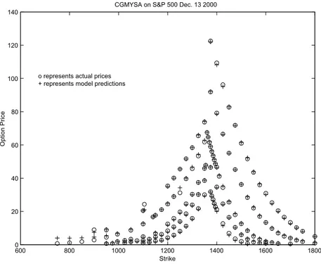
600 800 1000 1200 1400 1600 1800 0 20 40 60 80 100 120 140
CGMYSA on S&P 500 Dec. 13 2000
Strike
Option Price
o represents actual prices + represents model predictions
Figure 2: The ¯t of the model CGM Y SA to option price data for all atrikes and maturities on December 13 2000
regard.
The estimates for the volatility of the time change are consistent between N IGSA and CGMY SA with mean values of 5:34 and 6:97 respectively. The values are somewhat higher for V GSA at 16:45:
The best performing model by far is the CGM Y SA model, as it consistently has the lowest pricing errors. The parameters of this model are also more stable across
time. The mean pricing errors for the models N IGSA; V GSA; and CGMY SA are
4:1346%; 4:4251%; and 3:3738% respectively. Among the six models studied here, the tentatively best model is CGMY SA: The best overall ¯t was for December 13 2000 for CGMY SA; and we present a graph (see ¯gure (2)) of the actual and predicted prices for this day. However, it should be noted that lower dimensional calibrations are faster, and the improvements in ¯t may not warrant the extra time required for some applications.
7.2
Absolute Percentage Errors for the Year
For the three exponential models estimated for each of the twelve days in the year 2000, we stacked all of the absolute percentage pricing errors across strikes and maturities. The pricing errors are themselves orthogonal to strike and maturity, but the absolute pricing errors tend to be larger for shorter maturities and options which are further out-of-the-money. This is con¯rmed by regression results of the absolute errors on moneyness and maturity, where we employ moneyness and its square to capture the fact that we have out-of-the-money options on both sides of the forward. Table 7 presents the results.
We note that the quadratic in moneyness is signi¯cant in both its linear and quadratic terms. The shape is consistent with absolute errors rising as an option gets further out-of-the-money. The coe±cient for maturity is also negative and signi¯cant, which is
indicative of higher absolute errors for shorter maturity options. The R2 coe±cients are around 50% with values of 51:62; 49:07; and 47:12 for the models N IGSA; V GSA; and CGMY SA respectively.
7.3
Estimation Results for Other Underliers
For other underliers, we present a sample of quarterly estimates on the three dominating models N IGSA; V GSA; and CGM Y SA: For each model, we present results on ¯ve selected names. For NIGSA, results are presented for BKX, MCD, PFE, INTC and MSFT. For VGSA, we present result from RUT, GE, JNJ, IBM, and SUNW. Finally, from CGMYSA, results are given for DRG, HWP, BA, CSCO and ORCL. These results are presented in tables 8 through 10, one for each model.
The presence of skewness is once again consistently observed in the form of consistently negative values for µ in the case of N IGSA; and consistently lower values for G than M for the V GSA and CGMY SA models. Generally, the long term activity levels are lower than current activity levels, as re°ected in comparing the parameters C with the values ´: This is consistent with the view that volatilities over the year 2000 were on the high side. The performance of N IGSA and V GSA is quite good for options on single names. This may be a consequence of the fact that fewer options are available for calibration, with the result that the lower dimensional models are su±cient to capture their variation.
8
Comparative Results on Jump-Di®usion Models
In this section we outline some recent jump-di®usion models proposed by Bates [7] and Du±e, Pan, and Singleton [14](henceforth DPS). We also present some estimation results for these models on our data set. Bates' model is similar to our SV models in that the jump intensity is proportional to the level of a CIR process. In Bates' model, this process is also the volatility of the di®usion component in the stock. In addition, DPS allow for jumps in the volatility with an exponential density for the jump magnitude in volatility. Conditioning on a jump occurring, the Bates and DPS models both have a lognormally distributed jump in the stock price. Thus the resulting jump process for the log of the price has ¯nite activity and has a Levy density which is not completely monotone.
We focus on the following special case of the model by Bates, which is also studied by Pan [32]: dS(t) = (r¡ q ¡ ¸y¹)Stdt + p VtStdWS(t) + JyStdqy(t) dVt = (µv¡ ·vVt)dt + ¾v p VtdWV(t) dWSdWV = ½dt
(1 + Jy) is lognormally distributed with mean ¹y and variance ¾2y qy(t) is a Poisson process with arrival rate ¸yVt
¹ = (exp(¹y+ ¾2y=2)¡ 1): This model has eight parameters
We also focus on the following subset of the class studied by DPS [14]: dSt = (r¡ q ¡ ¸y¹)Stdt + p VtStdWS(t) + JyStdqy(t) dVt = ·v(µv¡ Vt)dt + ¾v p VtdWV(t) + JVdqv(t) dWSdWV = ½dt
(1 + Jy) is lognormally distributed with mean ¹y and variance ¾2y JV has an exponential distribution with mean ¹V
qy(t); qv(t) are independent Poisson processes with arrival rates ¸y; ¸v The parameter ¹ in the stochastic di®erential equation for the stock is de¯ned as in Bates. The model has ten parameters
V (0); ½; ¾v; ·v; µv; ¸y; ¹y; ¾y; ¹v; ¸v
Table 11 presents results on the Bates model estimated for every second Wednesday of each month, of the year 2000: Table 12 provides the results for the DPS models. We note that these models provide a competitive performance in summarizing the surface of option prices at a point of time.
9
Conclusion
Six stochastic volatility models were formulated by time changing three homogeneous L¶evy processes. The L¶evy processes employed were the normal inverse Gaussian model of Barndor®-Nielsen [4], the variance gamma of Madan, Carr, and Chang [27], and the CGMY model of Carr, Geman, Madan, and Yor [10]. The time change used to induce stochastic volatility was the integral of the CIR (Cox, Ingersoll and Ross [11]) process. This resulted in three process respectively termed N IGSV; V GSV; and CGMY SV: Mod-els for the stock price were built by exponentiating these processes and correcting the mean in accordance with spot forward arbitrage considerations, leading to the N IGSA; V GSA; and CGM Y SA models. A second class of discounted stock price models was obtained using stochastic exponentials, resulting in the N IGSAM; V GSAM;and CGM Y SAM models. These models imply that forward prices are martingales in the expanded ¯ltra-tion, which includes a knowledge of the integrated CIR time change process.
The paper also introduces two properties of stochastic processes, termed respec-tively the property of L¶evy marginals and the property of martingale marginals. The
N IGSV; V GSV; and CGMY SV processes satisfy the L¶evy marginal property when the
underlying CIR is started at zero. In this case, the resulting N IGSA; V GSA;and
CGMY SA processes have the property of martingale marginals. More generally, however, one may have the martingale marginal property for the SA processes, without having the L¶evy marginal property for the SV processes. We hope to devote some future research on these notions. In our view, the property of the existence of martingale marginal processes is fundamental at each time point for the risk neutral dynamics. Its application delivers a parametric model consistent with observed prices at each date, with parameters that will vary from day to day. The arbitrage-free risk-neutral dynamics is to be sought in the higher dimensional ¯ltration of the asset price and the parameters of the synthesizing martingale marginal processes.
The six models were estimated for every second Wednesday of the month for each month of the year 2000 on data for S&P 500 options and 20 other underlying assets. For the S&P 500 options, the exponential models were signi¯cantly better than their stochastic exponential counterparts in all 3 cases, suggesting that this may be the general
preferred direction. The results for the S&P 500 index options consistently re°ected market skews, and stochastic volatility, with mean reversion rates of around seven weeks. Similar patterns were observed for other underliers.
The best model by far was the CGMY SA model, with percentage errors across all strikes and maturities reaching as low as 2% for the S&P 500 index options. For options on single names, the performance of the lower dimensional NIGSA and V GSA models was adequate. The class of models proposed here is for the ¯rst time providing us with a relatively parsimonious representation of the surface of option prices, with some stability over time in the parameter estimates. Results on competing models in the jump-di®usion class are also provided. These structures lead to interesting applications on pricing exotic products and analysing risk management strategies in empirically realistic, yet tractable contexts. We expect continuing research to shed further light on these interesting ques-tions. Of particular interest is the study of the statistical dynamics in the same parametric class, which would lead to explicit representations of the measure change process and its representation of risk pricing in ¯nancial markets.