RATEMAKING TERRITORIES AND ADVERSE SELECTION RISK FOR FLOOD INSURANCE
DISSERTATION PRESENTED
AS PARTIAL REQUIREMENT TO THE MASTER IN MATHEMATICS
BY
MARIA ANGELICA OJEDA DAVILA
TERRITOIRES DE TARIFICATION ET RISQUE D’ANTISÉLECTION EN ASSURANCE INONDATION
MÉMOIRE PRÉSENTÉ
COMME EXIGENCE PARTIELLE DE LA MAÎTRISE EN MATHÉMATIQUES
PAR
MARIA ANGELICA OJEDA DAVILA
UNIVERSITÉ DU QUÉBEC À MONTRÉAL Service des bibliothèques
Avertissement
La diffusion de ce mémoire se fait dans le respect des droits de son auteur, qui a signé le formulaire Autorisation de reproduire et de diffuser un travail de recherche de cycles
supérieurs (SDU-522 – Rév.10-2015). Cette autorisation stipule que «conformément à
l’article 11 du Règlement no 8 des études de cycles supérieurs, [l’auteur] concède à l’Université du Québec à Montréal une licence non exclusive d’utilisation et de publication de la totalité ou d’une partie importante de [son] travail de recherche pour des fins pédagogiques et non commerciales. Plus précisément, [l’auteur] autorise l’Université du Québec à Montréal à reproduire, diffuser, prêter, distribuer ou vendre des copies de [son] travail de recherche à des fins non commerciales sur quelque support que ce soit, y compris l’Internet. Cette licence et cette autorisation n’entraînent pas une renonciation de [la] part [de l’auteur] à [ses] droits moraux ni à [ses] droits de propriété intellectuelle. Sauf entente contraire, [l’auteur] conserve la liberté de diffuser et de commercialiser ou non ce travail dont [il] possède un exemplaire.»
First of all, I would like to thank my research director Mathieu Boudreault for his support in my academic journey since my arrival in Canada. I offer him my sincere appreciation for his availability, his patience, and his advice, which were essential to conducting this research. I would also like to express my gratitude to The Co-operators and the Canadian Institute of Actuaries who supported this project through the Mitacs Accelerate Program.
I would like to thank my partner Marcelo for his continual support throughout this entire project and his confidence in me. Finally, I thank my daughter Valentina for keeping me company throughout this experience.
LIST OF TABLES . . . vii
LIST OF FIGURES . . . ix
RÉSUMÉ . . . xiii
ABSTRACT . . . xv
INTRODUCTION . . . 1
CHAPTER I CLUSTERING METHODS . . . 5
1.1 Principles . . . 6
1.2 Types of Clustering Methods . . . 9
1.3 K-Means Clustering . . . 12
1.4 Hierarchical Clustering . . . 15
1.5 Hybrid Clustering . . . 20
1.6 SKATER . . . 20
1.7 Measures of Cluster Quality . . . 26
CHAPTER II APPLICATIONS OF CLUSTERING METHODS TO FLOOD RISK . . . 27
2.1 Data . . . 27
2.1.1 Digital Terrain Model (DTM) . . . 28
2.1.2 Flood Hazard Maps . . . 29
2.1.3 Rivers . . . 31 2.1.4 Damage Curve . . . 32 2.2 Data Transformation . . . 33 2.3 Applications . . . 35 2.3.1 K-Means Clustering . . . 38 2.3.2 Hierarchical Clustering . . . 49
2.3.3 SKATER Clustering . . . 56
CHAPTER III ECONOMIC AND ACTUARIAL ANALYSES OF AD-VERSE SELECTION RISK . . . 63
3.1 Other Clustering Methods . . . 63
3.1.1 Forward Sortation Area-Based Clustering . . . 64
3.1.2 Dissemination Area-Based Clustering . . . 65
3.1.3 Floodplain-Based Clustering . . . 68
3.2 Comparison Between Statistical, Geopolitical, and Floodplain-Based Clustering Approaches . . . 70
3.3 Adverse Selection Risk Analysis . . . 72
CONCLUSION . . . 81
APPENDIX A DATA . . . 83
APPENDIX B DATA TRANSFORMATION PROCEDURE . . . 89
APPENDIX C DISTRIBUTION OF CLUSTERS . . . 91
Table Page 0.1 Main Flood Events in Canada from 2017 to 2019 . . . 2 2.1 Descriptive Statistics of Clusters Using K-Means Clustering Method
Based on Flood Losses . . . 42 2.2 Descriptive Statistics of Clusters Using K-Means Clustering Method
Based on Flood Losses and Location . . . 47 2.3 Descriptive Statistics of Clusters Using Hierarchical clustering Based
on Flood Losses . . . 54 2.4 Descriptive Statistics of Clusters Using SKATER Clustering . . . 59 3.1 Comparison FSA-Based Clustering and K-Means Clustering (Four
Clusters) . . . 74 3.2 Comparison FSA-Based Clustering and Hierarchical Clustering (Five
Clusters) . . . 74 3.3 Comparison Floodplain-Based Clustering and K-Means Clustering
(Four Clusters) . . . 76 3.4 Comparison Floodplain-Based Clustering and K-Means Clustering
(Ten Clusters) . . . 77 3.5 Comparison Floodplain-Based Clustering and Hierarchical
Cluster-ing (Ten Clusters) . . . 78 3.6 Comparison K-Means Clustering (Ten Clusters) and Hierarchical
Figure Page
1.1 K-Means Clustering Algorithm with K=2, Part I . . . 13
1.2 K-Means Clustering Algorithm with K=2, Part II . . . 14
1.3 Hierarchical Clustering Algorithm, Part I . . . 18
1.4 Hierarchical Clustering Algorithm, Part II . . . 19
1.5 SKATER Clustering Algorithm, Part I . . . 23
1.6 SKATER Clustering Algorithm, Part II . . . 24
1.7 SKATER Clustering Algorithm, Part III . . . 25
2.1 DTM of the Study Area - 25-Meter Resolution . . . 29
2.2 The City of Calgary, Alberta, Canada . . . 31
2.3 Damage Curve for One Storey House with Finished Basement . . 33
2.4 Expected Flood Loss (%) - 25-Meter Resolution . . . 34
2.5 Expected Flood Loss (%) - 250-Meter resolution . . . 35
2.6 Elbow Plot of Statistical-Based Clustering Methods . . . 37
2.7 Spatial Distribution of Clusters Considering 4 and 10 Groups Based on Flood Losses - K-Means Algorithm . . . 40
2.8 Boxplots of Clusters Considering 4 and 10 Groups Based on Flood Losses - K-Means Algorithm . . . 41
2.9 Distribution of the Difference Between the Expected Premium Col-lected and the True Expected Loss for 4 (Top) and 10 (Bottom) Groups Based on Flood Losses - K-Means Algorithm . . . 43
2.10 Spatial Distribution of Clusters Considering 5 and 10 Groups Based on Flood Losses and Location - K-Means Algorithm . . . 45
2.11 Boxplots of Clusters Considering 5 and 10 Groups Based on Flood Losses and Location - K-Means Algorithm . . . 46 2.12 Distribution of the Difference Between the Expected Premium
Col-lected and the True Expected Losses for 5 (Top) and 10 (Bottom) Groups Based on Flood Losses and Location - K-Means Algorithm 48 2.13 Dendrogram of Hierarchical Clustering Method Considering Flood
Losses Using Complete Linkage . . . 50 2.14 Spatial Distribution of Clusters Considering 5 and 10 Groups Based
on Flood Losses - Hierarchical Algorithm . . . 52 2.15 Boxplots of Clusters Considering 5 and 10 Groups Based on Flood
Losses - Hierarchical Algorithm . . . 53 2.16 Distribution of the Difference Between the Expected Premium
Col-lected and the True Expected Losses for 5 (Top) and 10 (Bottom) Groups Based on Flood Losses - Hierarchical Algorithm . . . 55 2.17 Spatial Distribution of Clusters Considering 7 and 10 Groups Based
on Flood Losses and Location - SKATER Algorithm . . . 57 2.18 Boxplots of Clusters Considering 7 and 10 Groups Based on Flood
Losses and Location - SKATER Algorithm . . . 58 2.19 Distribution of the Difference Between the Expected Premium
Col-lected and the True Expected Losses for 7 (Top) and 10 (Bottom) Groups Based on Flood Losses and Location - SKATER Algorithm 60 3.1 Spatial Distribution of Clusters Based on FSA (Top) and DA
(Bot-tom) . . . 66 3.2 Boxplots of Clusters Based on FSA (Top) and DA (Bottom) . . . 67 3.3 Floodplain-Based Clustering Approach - Spatial Distribution of
Clusters (Top) and Distribution of Expected Loss by Clusters (Bot-tom) . . . 69 3.4 Elbow Plot of Selected Clustering Methods, Geopolitical, and Floodplain-Based Clustering Approaches . . . 71 A.1 Alberta Data Terrain Model - 25-Meter Resolution . . . 83
A.2 Floodplains of 5-Year (Top) and 10-Year (Bottom) Return Period over Alberta DTM . . . 84 A.3 Floodplains of 20-Year (Top) and 50-Year (Bottom) Return Period
over Alberta DTM . . . 85 A.4 Floodplains of 100-Year (Top) and 200-Year (Bottom) Return
Pe-riod over Alberta DTM . . . 86 A.5 The Bow River and Elbow River over Alberta DTM . . . 87 C.1 Spatial Distribution of Clusters Considering 4 and 10 Groups Based
on Flood Losses and Location - Hierarchical Algorithm . . . 92 C.2 Boxplots of Clusters Considering 4 and 10 Groups Based on Flood
Losses and Location - Hierarchical Algorithm . . . 93 C.3 Spatial Distribution of Clusters Considering 4 and 10 Groups Based
on Flood Loss - Hybrid Algorithm . . . 94 C.4 Boxplots of Clusters Considering 4 and 10 Groups Based on Flood
Losses - Hybrid Algorithm . . . 95 C.5 Spatial Distribution of Clusters Considering 5 and 10 Groups Based
on Flood Losses and Location - Hybrid Algorithm . . . 96 C.6 Boxplots of Clusters Considering 5 and 10 Groups Based on Flood
Les primes d’assurance inondations doivent refléter le risque réel auquel sont con-frontés les propriétaires, c’est pourquoi il est nécessaire de différencier les risques afin d’éviter ou de minimiser le risque de sélection adverse (ou antisélection). Toutefois, cela pourrait entraîner de grandes variations spatiales des primes, car la topographie et la proximité des cours d’eau ont une influence importante dans la détermination de la prime. Dans ce projet, différentes méthodes de regroupement (clustering) sont appliquées pour identifier les endroits présentant un potentiel de perte similaire en raison du risque d’inondation, ce qui est important pour les (ré)assureurs à des fins de tarification et de souscription. Nous avons constaté que les territoires de tarification non contigus sont plus homogènes, avec des variations sensiblement plus faibles des pertes estimées à l’intérieur de ces territoires de tar-ification. Plus précisément, nous avons constaté que les territoires de tarification basés sur le code postal ne fonctionnent pas pour différencier les risques, comme prévu. Également, les regroupements basés sur les plaines inondables ignorent les effets de la profondeur de l’eau dans la distribution des pertes, ce qui ajoute une variance significative au sein de leurs territoires. Il a été démontré que les approches de regroupement basées sur les statistiques permettent de définir des territoires de tarification dans des régions géographiques beaucoup plus vastes, y compris des zones qui pourraient autrement être exclues ou dont la couverture serait très coûteuse. Les résultats sont analysés par la quantification du risque d’antisélection selon différents scénarios et cela montre l’importance d’investir dans des cartes d’inondations précises à haute résolution.
MOTS CLÉS : Risques d’inondation, Méthodes de clustering, Territoires de tarifi-cation, Territoires basés sur les risques d’inondation, Cartes des risques d’inondation.
Flood insurance premiums should reflect the true risk that homeowners face, there-fore, differentiation between risk is necessary to avoid or minimize adverse selection risk. However, this might lead to large spatial premium variations because the topography and proximity to water bodies have a prominent influence in the deter-mination of the premium. In this project, different clustering methods are applied to identify locations with similar expected loss potential due to flood risk, which is important for (re)insurers for ratemaking and underwriting purposes. We found that territories with non-contiguous constraints are more homogeneous, with sig-nificantly lower variations of estimated losses within them, compared with terri-tories created under geopolitical restrictions or floodplain clustering approaches. Specifically, we found that ratemaking territories based on postal code do not work well to differentiate risks, as expected, as well as floodplain-based clustering since the latter ignores the effects of water depth in the loss distribution adding sig-nificant variance within their territories. It has been shown that statistical-based clustering approaches allow ratemaking territories to be defined in much wider geographic regions including zones that could otherwise have been excluded or be very expensive to be insured. The results are analysed through the quantification of the adverse selection risk under different scenarios which shows the value of investing in accurate flood hazard maps.
Keywords: Flood risk, Clustering methods, Ratemaking territories, Flood risk-based territories, Flood hazard maps.
Floods are among the natural disasters that cause large economic losses around the world; they are also one of the most recurrent, and are expected to increase in frequency and intensity due to the effects of climate change. Floods occur frequently across Canada, most often caused by spring thaw and heavy storm rainfall (OECD & The World Bank, 2019) and are the costliest in terms of property damage (Public Safety Canada, 2015).
The last largest single flood event in Canada occurred in Calgary in the sum-mer of 2013. The estimated total cost was CAD 2.7 billion of which 37 percent was covered by the federal government through the Disaster Financial Assistance Arrangements (DFAA), as reported by the Canadian Disaster Database.
In the last three years, Canada has however faced significant insured losses caused by smaller severe weather events like floods, rain, snow, and windstorms. Accord-ing to the Insurance Bureau of Canada, these losses were estimated at CAD 1.3 billion in 2019, CAD 2.1 billion in 2018, and CAD 1.25 billion in 2017, considered to be, respectively, the seventh, fourth, and ninth-highest losses on record. So far in 2020, the flood in Fort McMurray alone has cost the industry CAD 522 million, and insured losses from severe weather in Alberta have been estimated at over CAD 2 billion (Insurance Bureau of Canada, 2020). The main flood events that contribute to insured losses mentioned before are shown in Table 0.1.
It is important to mention that most of the consequences derived from floods in Canada have been assumed by the government through the DFAA, a federal pro-gram that provides financial assistance to provincial and territorial governments
Table 0.1 Main Flood Events in Canada from 2017 to 2019
Description Region Year Insured Losses
Spring floods Ontario and Quebec 2017 CAD 223 million Spring floods Quebec and New Brunswick 2019 CAD 208 million
Flood Toronto August 2018 CAD 80 million
Storms and floods Southern Ontario and Quebec February 2018 CAD 57 million Storms and floods Eastern Canada January 2018 CAD 54 million
in the event of a large-scale natural disaster. This assistance is not paid directly to affected individuals, small businesses, or communities but to the provinces or ter-ritories, in excess of what they could reasonably be expected to bear themselves, based on their population (Public Safety Canada, 2020). According to the Office of the Parliamentary Budget Officer (2016), considering the DFAA payments from 1970 to 2014, 78% were made in response to floods; the provinces of Alberta and Quebec were the main recipients with 28% and 25% of all payments, respectively. Flood insurance offered by private insurers started in 2015 as an endorsement to home insurance. However, in the past and despite a lack of flood risk coverage, insurers often ended up paying for flood-related damage in the event of major floods, this was due to difficulty in ascertaining the causes of loss and a desire to avoid reputational risk during major flood disasters (Davis et al., 2018). In Quebec, limited flood insurance became available in 2018 (OECD & The World Bank, 2019). As of spring 2019, the take-up rate of overland flood insurance in Canada is estimated at 34 percent, and 77 percent of those insurance products were offered by sixteen insurers (Insurance Bureau of Canada, 2019).
on Financial Management of Flood Risk was created to study the options of transferring residential property flood risk from public sector, funded by taxpayers, to private sector insurance solutions, funded by the property owners, as stated in Insurance Bureau of Canada (2019).
In June 2019, the National Working Group on Financial Risk of Flooding, as previously mentioned, proposed three solutions where the insurance market is involved in different ways. These options are, first, the creation of a high-risk flood insurance pool which would include high flood risk properties that are not normally considered an insurable risk. The second option is the blend of risk sharing between homeowners and the government, where the private sector would take flood risk according to its risk appetite leaving high flood risk properties to be covered ex post by government DFAA programs, which is more or less the status quo, and the third option is a pure market solution where properties are no longer covered by DFAA programs and homeowners either self-insure, move, or transfer their risk to the private insurance market.
In all cases, the private insurance market is involved, meaning that flood insurance premiums should reflect the true risk that homeowners face through the differen-tiation between risks in the underwriting policies and ratemaking methodologies. Differentiation between risks allows the insurers to avoid or minimize the ad-verse selection risk, which is the result of overcharging low-risk policyholders and undercharging high-risk policyholders, which would in turn attract high-risk pol-icyholders, causing important future losses.
However, perfect differentiation between risks might also lead to premiums with large spatial variations due to changes in elevation in relatively small areas in some territories and proximity to water bodies (Davis et al., 2018). This limitation is also noted in Boudreault et al. (2019), wherein they report finding a large
heterogeneous spatial distribution of the relativities due to the topography of the terrain and how the river overflows in the calculation of premiums and ratemaking territories definitions.
To overcome this limitation of large spatial variations of risks, Davis et al. (2018) propose grouping risks by similar loss costs rather than create pricing territories by contiguous boundaries, e.g., postal codes, neighborhoods, etc. This approach has the advantage of reducing the variation of premiums, consequently the estimated losses within a territory will be more homogeneous. Flood ratemaking territories thus implies a trade-off between loss cost homogeneity and location similarity. The general objective of this thesis is to apply some classical and spatial constraint clustering methods to define ratemaking territories with similar flood risk profiles so that we can find an equilibrium between the true premium and the one that leads to adverse selection risk. In addition, we will select the optimal number of territories to differentiate between them. Furthermore, to have a more stable long-term view of anticipated losses that may arise in future, notional exposure data is used by placing multiple notional policy records at each geographic location in the city of Calgary to eliminate exposure, policy attributes, and building characteris-tics bias in the analysis. One specific objective is to quantify the adverse selection risk that results from creating ratemaking territories under different scenarios. This thesis is organized as follows: in Chapter 1, we look at different clustering methods that allow us to smooth out the spatial distribution of flood insurance premiums. In Chapter 2, a description of the data and applications of clustering methods is presented. Chapter 3 presents an economic analysis of the resulting composition of an insurer’s portfolio against competing insurers, having different ratemaking territories, in a market where policyholders are rational, seeking the lowest premium. Finally, a brief conclusion completes this document.
CLUSTERING METHODS
Clustering is an unsupervised learning technique that allows us to discover struc-tures in a data set by creating groups or clusters, without having a response variable. In fact, clustering methods allow a better understanding of the data instead of finding a right answer, because there is no response variable to evaluate their performance.
Clustering is used for grouping or arranging observations with similar features into groups, or for grouping features to discover groups among them on the basis of the observations (James et al., 2013).
Different clustering methods allow us to group observations. The objective of this study is to cluster homeowners with similar flood risk profiles in the city of Calgary, Alberta, Canada.
In this chapter, we introduce the guiding principles of clustering methods, which are based on Hastie et al. (2009), and summarise some of the classical and spatial clustering methods and the implications when working with spatial data. After-wards, we will present, in detail, some of the most commonly used methods in practice as well as a spatial clustering algorithm.
1.1 Principles
The main principle of clustering methods is to group similar observations into groups, so that the observations within each group are similar to each other, while the observations in different groups are different from each other (James et al., 2013). It is important to mention, that each observation can only belong to one cluster.
More precisely, the objective is to separate the set X of N observations, i.e., X = {x1, x2, x3, ..., xN}, into K clusters (C1, C2,...,CK), where Ck is a subset of X, and the observations falling within a given cluster are similar such that:
• SK
k=1Ck = X,
• Ck\ Ck0 =; for all k 6= k0,
• K < N.
Fundamental to all clustering methods is the selection of distance or dissimilarity measure, or similarity measure, between two observations (Hastie et al., 2009). The most common dissimilarity measure used between observations xi and xi0 is
the squared Euclidean distance expressed as D(xi, xi0) = kxi xi0k2. Although
other measures can be used such as absolute difference distance, correlation-based distance, rank correlation, Manhattan distance (also known as City-Block dis-tance), etc. From a theoretical viewpoint, it is best to use the Euclidean distance for the K-means algorithm, and the City-Block distance for K-medians, as stated by de Hoon et al. (2003).
Usually, the observations have p features, variables, or attributes, i.e., xi = {xi1, xi2, xi3, ..., xip}; then, each observation can be viewed as a tuple (list of fea-tures) and the distance between observations is defined as
D(xi, xi0) =
p X j=1
dj(xij, xi0j),
where dj(xij, xi0j)is the distance between values of the feature j of the observation i. Specifically, when the dissimilarity measure is the squared Euclidean distance, the distance between observations is defined as
D(xi, xi0) =
p X j=1
(xij xi0j)2. In general, the distance between observations is expressed as
D(xi, xi0) = p X j=1 wjdj(xij, xi0j), where Pp
j=1wj = 1 and wj reflects the relative importance of the attributes. For further details see Hastie et al. (2009).
When looking at the principle of grouping similar observations, the objective is achieved by maximizing within-cluster similarity. This objective could be alterna-tively expressed as: minimizing within-cluster dissimilarity, maximizing between-cluster dissimilarity, or minimizing between-between-cluster similarity.
Since the goal is to assign close points to the same cluster, a natural loss function, as stated in Hastie et al. (2009), would be the total within-cluster variation
W (C) = 1 2 K X k=1 X C(i)=k X C(i0)=k D(xi, xi0) = K X k=1 W (Ck),
where each observation is assigned to only one cluster through the encoder k = C(i), that assigns the ith observation to the kth cluster. Therefore, we want to minimize the total within-cluster variation.
The total within-cluster variation is the sum of overall K clusters within-cluster variation W (Ck). It is also referred to as within-cluster point scatter.
The between-cluster variation, also known as between-cluster point scatter, is defined as B(C) = 1 2 K X k=1 X C(i)=k X C(i0)6=k D(xi, xi0).
The total point scatter or total variance is defined as
T = 1 2 N X i=1 N X i0=1 D(xi, xi0) = 1 2 K X k=1 X C(i)=k 0 @ X C(i0)=k D(xi, xi0) + X C(i0)6=k D(xi, xi0) 1 A, or T = W (C) + B(C),
which is constant given the data, independent of cluster assignment. Then, mini-mizing within-cluster variation or dissimilarity W (C) is equivalent to maximini-mizing between-cluster dissimilarity B(C), as outlined above.
These measures and the cluster distributions allow us to assess the degree of difference between the clusters to determine if the data is appropriately clustered in a set of different groups.
Clustering is a combinatorial optimization problem because it involves finding groups of objects that satisfy given conditions. It has an input and an objective defining the properties of the solution. However, there are computational chal-lenges because there are KN possible arrangements to group N observations in K clusters. Therefore, it is not possible to do this exhaustively. To come up with a solution, different algorithms are considered; though they do not guarantee the global optimum solution, they do end up with a local optimum solution.
1.2 Types of Clustering Methods
Classical clustering methods are classified into four main categories: partitioning methods, hierarchical methods, density-based methods, and grid-based methods. A number of clustering methods can be adapted to or are specially tailored for spatial data (Neethu & Surendran, 2013) and, depending on real life constraints such as physical or operational, these methods can be modified into constraint-based clustering methods (Han et al., 2001).
Among partitioning methods, where the number of clusters is specified from the beginning, K-means is the most well known clustering method that defines groups by their center. But there are others methods like K-medians, K-medoids, and Expectation Maximization algorithm (EM). For example, the latter and Fuzzy C-means are the most prevalent methods for automatic segmentation of magnetic resonance brain images and, recently Prakash & Kumari (2017), have incorporated spatial information and bias correction to overcome some problems.
Hierarchical methods, unlike partitioning methods, do not require pre-specifying the number of groups but, instead, they decompose data in a hierarchical struc-ture. The most traditional methods are bottom-up clustering, where the algorithm starts by placing each observation in its own cluster, and top-down clustering where it, as opposed to the former method, starts by placing all objects in one group. Other methods in this category are: BIRCH (Balanced Iterative Reducing and Clustering Using Hierarchies), CURE (Clustering Using Representatives), and CHAMALEON (Karypis et al., 1999). Regarding a constraint-based clustering of these methods, Chavent et al. (2018) propose a hierarchical clustering algorithm with soft contiguity constraint called HCLUSTGEO. Although it includes a spa-tial constraint, it is not considered a spaspa-tial clustering method because it does not always result in compacted groups.
Density-based clustering methods find groups based on the locations of the obser-vations. Among these methods are DBSCAN (Density-Based Spatial Clustering of Applications with Noise), HDBSCAN (Hierarchical DBSCAN), OPTICS (Or-dering Points to Identify the Clustering Structure) and DENCLUE (Clustering based on Kernel Density Estimation). These methods are more influenced by the spatial distribution of the observations looking for density regions to regroup them, which are separated for low density observations labeled as noise. These clustering methods can be used to filter outliers and discover clusters of arbitrary shapes.
Grid-based clustering methods are a way to increase the efficiency of density-based clustering methods by quantizing dense regions into a finite number of cells and perform the algorithm in the quantized space (Neethu & Surendran, 2013). Al-though these methods are more efficient, they decrease effectiveness as they use summarized information. Among these methods are STING (Statistical Informa-tion Grid approach), Wave Clustering (Clustering using Wavelet TransformaInforma-tion), and CLIQUE (CLustering in QUEst).
When working with spatial data, we can apply classical clustering methods to group the observations based only on features and see the natural patterns that emerge in a map, or we can just group them based on their spatial location. In the latter approach, a density-based clustering method is usually applied while in the former approach, these methods are used to help us in finding patterns that would otherwise go unseen.
Furthermore, to include geographical information in the optimization process of classical clustering methods, the coordinates x and y can be included as additional attributes, as proposed by Haining et al. (2000). Even though this method tends to yield more geographically compacted clusters, it does not guarantee contiguity
(Anselin et al., 2006).
However, clustering methods that aim to group the observations based on the attributes’ similarity and on condition the observations can be grouped only when contiguous, are called spatial clustering methods.
Spatial contiguity is a very important constraint in clustering. It is well known from the literature on contiguity constrained spatial clustering that neighbors in attribute space are not necessarily neighbors in geographic space Anselin (2019). Consequently, spatial clustering is based on attribute similarity and location sim-ilarity.
The objective of the spatial clustering methods is not for exploratory purpose; they are used for creating regions that contain similar observations in terms of attributes that are geographically similar in terms of location, or for creating a spatial variable for another model.
Some spatial clustering methods are: SKATER (Spatial ‘K’luster Analysis by Tree Edge Removal) developed by Assunção et al. (2006), max-p regions problem (Duque et al., 2012), and REDCAP (Kupfer et al., 2012), among others. Re-cently, Wang (2018) developed a method that proposes a CHAMALEON spatial hierarchical clustering method with a contiguous constraint in areal data.
Clustering methods have a large variety of applications in different fields like marketing, medicine, biostatistics, bioinformatics, finance, actuarial science, etc. In this thesis, we apply some of these methods to group homeowners (observations) based on the similarity of their expected loss (feature) due to flood risk.
In the following section, we present three classical clustering methods as well as a spatial clustering algorithm.
1.3 K-Means Clustering
Partitioning clustering methods essentially define groups by their center. This method aims to group the data in K distinct groups where each cluster center is defined as the mean of all the observations in that respective cluster.
As mentioned before, clustering is an optimization problem where we look to minimize the within-cluster variation, which can be expressed as
W (C) = K X k=1 Nk X i=1 D(x(k)i , ¯xk),
where Nk is the number of observations in the cluster Ck, ¯xk is the mean vector associated with that cluster, and x(k)
i is the ith observation of that kth cluster. Therefore, minimizing the loss function means finding the centers (¯x1, ..., ¯xK) in such a way that the total distance from each center to within-group observations is as small as possible.
The algorithm consists of the following steps:
1. Initialization: start with random assignments of all observations into K groups, where K is set in advance.
2. Finding the cluster centers: the cluster centers are calculated as the mean over all the observations in a cluster for each attribute.
3. Assigning observations to the closest center: determine, for each observation, which cluster is closest and then assign each one to the respective cluster. 4. Repeat Steps 2 and 3 until the cluster centers no longer change, i.e., until
We will apply this algorithm to a data that has 200 observations in two-dimensional space. Figures 1.1 and 1.2 show the progress of the K-means algorithm with K=2. The data is shown at the top of Figure 1.1, at the middle it shows how each observation is randomly assigned to a cluster, and then at the bottom, the cluster centers are computed. Figure 1.2, at the top, shows the assignments of the observations to the nearest center to then calculate the new cluster centers. This process is repeated until the algorithm converges, the result is shown at the bottom of this figure.
It is important to mention that, as outlined in Section 1.1, the K-means algorithm finds a local rather than a global optimum; this method is sensitive to the starting point (the initialization step).
Actually, when the data has outliers, this algorithm could let them become their own cluster and the cluster center will never move closer to actual data; we then end up with an unrepresentative cluster with only one or few observations nowhere near the rest of the data.
Therefore, to mitigate this disadvantage, different starting points are tested, and the solution that gives the minimum total within-cluster variation is selected as an approximation of the global optimal solution.
1.4 Hierarchical Clustering
Hierarchical clustering methods build a hierarchy of clusters without specifying the number of clusters in advance. In these methods, clusters are created based on the distances between observations and distances between clusters. These distances are represented in the form of a tree structure called a dendrogram. Distances between observations have already been mentioned, but these types of
clustering methods also require distances between clusters to continue comparing similarities, also known as linkage, and can be defined in several ways.
The most common types of dissimilarity between clusters, as stated by de Hoon et al. (2003), are: complete, also known as maximum, average, single, and centroid linkage, which differ in how the distance between clusters is defined in terms of their members.
Pairwise complete-linkage clustering defines the distance between two clusters as the longest distance among the pairwise distances between observations of the two clusters, which tends to yield more balanced clusters (James et al., 2013) and is the most used.
Pairwise single-linkage clustering defines the distance between two clusters as the shortest distance among the pairwise distances between the observations of the two clusters. In practice, in most situations, single linkage will not be a good choice, unless the objective is to identify a lot of singletons.
Pairwise average-linkage clustering defines the distance between two clusters as the average over all pairwise distances between the observations of the two clusters. It also tends to yield more balanced clusters as in complete linkage.
Finally, pairwise centroid-linkage clustering defines the distance between two clus-ters as the distance between the arithmetic means of the two clusclus-ters, also used in K-means clustering.
It is important to mention that the first three linkages can be formed directly from the dissimilarity matrix, which contains all the distances between the observations to be grouped, e.g., squared Euclidean distance can be used to create the matrix. Therefore, when using these linkages, there is no need to resort to the original data. In contrast, when using centroid-linkage, the cluster centres depend on the
mean of the observations, therefore original data is needed.
Generally, these hierarchical methods are used when hierarchy structure is ex-pected. In this thesis, the data has somewhat of a hierarchical structure consid-ering that if a property is affected by a 10-year flood, it will also be affected by floods having larger return periods. In the following chapter, we talk more about the data used in this thesis.
In this thesis, we have applied a bottom-up approach, and the algorithm consists of the following steps:
1. Calculate the distance matrix between the observations.
2. Group the two closest observations and they will form a cluster.
3. Determine the next closest pair, including the existing cluster in the compar-isons. The dissimilarity between clusters, or linkage, indicates the distance between nodes at each level to form the dendrogram.
4. Repeat Step 3 until all the observations have been included. The result is a dendrogram.
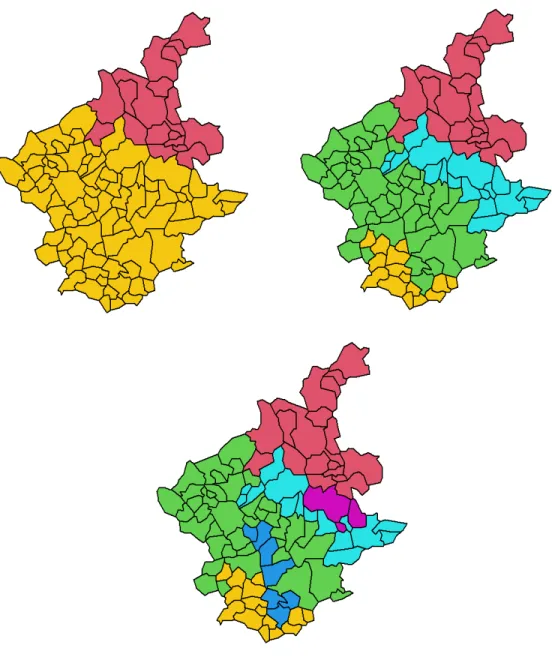
We will apply this clustering method to the data used in the previous section considering Euclidean distances between observations and complete linkage dis-tance between clusters. Figure 1.3 shows the structure of the data and how the observations are arranged in the dendrogram, a tree-like visual representation of the observations. We can see how many clusters and how they are formed when we cut the dendrogram at height of 4.1, 3, and 2.6. The height of the cut to the dendrogram plays the same role as the K in K-means clustering, it controls the number of clusters obtained.
Figure 1.4 shows how the observations are clustered into two dimensions. We can see at the top, that clustering the data into two groups find a quite different groups than clustering the data into three or four groups, for example.
1.5 Hybrid Clustering
The Hybrid approach considers the clustering methods outlined above, K-means and Hierarchical clustering approaches, used in conjunction with each other. That is, the dendrogram can be explored to find a good cut-point, and we can then use this value to find the number of clusters that the K-means clustering method needs as an input.
The algorithm consists of the following steps:
1. Compute hierarchical clustering and produce the dendrogram. 2. Cut the tree into K clusters.
3. Compute the cluster centers of each cluster, i.e., the mean of the observations of the clusters. This step would replace the initialization step of the K-means algorithm.
4. Follow the K-means clustering algorithm by using the set of cluster centers already calculated, as the initial cluster centers.
1.6 SKATER
The objective of spatial clustering methods is to create regions that need to be contiguous. The SKATER algorithm is based on pruning a minimum spanning tree (MST) constructed from the contiguity structure of the observations that need
to be clustered. This method creates groups of spatially connected observations that are similar in attributes.
The first step of this algorithm is to create a connectivity graph that captures the neighborhood, or adjacency, relationship between spatial observations. The connectivity graph shows the observations, represented by vertices, linked by edges to its neighbours. The cost of each edge measures the dissimilarity between the observations it joins.
The second step summarizes the connectivity graph by creating a MST which is a spanning tree with minimum cost. The cost is measured as the sum of dissimilarities over all edges of the tree. The spanning tree is a simplified version of the connectivity graph where any two observations are connected by a unique path, and the number of edges is N 1, i.e., the N observations are connected by N 1 edges.
In the third step, we prune the MST to create clusters. We start to prune the MST on the edge, or branch, that produces the largest between-cluster dissimilarity, which is the objective function. Then, the tree that generates the highest objective function is split successively until we obtain the number of clusters desired. The algorithm consists of the following steps:
1. Build the connectivity graph.
2. Construct a minimum spanning tree.
3. Prune the minimum spanning tree to maximize the between-cluster dissim-ilarity.
Figures 1.5, 1.6 and 1.7 show an illustration of the SKATER algorithm applied to a spatial data that has ninety eight polygons and an attribute variable called Economic Life Condition Index, i.e., each polygon, or areal unit, has an economic index. The data can be found in the R package called spdep (Bivand & Wong, 2018). The objective is to find regions by grouping similar areal units in terms of its economic life condition index.
Figure 1.5 shows, at the top left, the areal units to be analyzed and the contiguity structure of the data is shown at the right. This contiguity structure is reduced to a MST, shown at the bottom. The MST is a subset of the previous graph that includes all the nodes in the network connected without any cycles and with the minimum possible total edge cost.
Figure 1.6 shows how the MST is pruned to obtain two, four and six regions. For example, to obtain two regions, we remove one edge from the original MST, while three and five edges were removed to obtain four and six regions, respectively. Therefore, we can see two, four and six disconnected clusters in different colors. Finally, in Figure 1.7, we can see compacted regions, formed by areal units with similar economic indexes.
As we can see, the spatial contiguity constraint is always guaranteed in this method because the MST was created from the contiguity structure. This method uses a hierarchical division strategy because, at the beginning, all objects belong to a single tree. A disadvantage of this method is that when an observation ends up on a pruned branch of the tree, it cannot switch back to a previous branch; therefore, a local optimum could be found instead of a global one.
1.7 Measures of Cluster Quality
Choosing the best number of clusters is not straightforward. For example, K-means should be run with different numbers of clusters (K). The selected number would be determined after seeing the results and using the elbow plot, by looking at the percentage of variance explained as we add each new cluster. Hierarchical clustering methods allow us to select the number of clusters at the end of the process (James et al., 2013).
In practice, we try several different options and look for the one with the most useful or interpretable solution. With these methods, there is no single right answer; any solution that exposes any interesting aspects of the data should be considered (James et al., 2013).
In this thesis, we will use the elbow plot to select the optimal number of clusters. Specifically, we stop adding clusters when the additional explained variance be-comes small and use visual inspection of the elbow plot, because sometimes the growth of the variance explained is not smooth, and we can make important gains with two or three more clusters, for example.
APPLICATIONS OF CLUSTERING METHODS TO FLOOD RISK
The objective of this chapter is to analyse the performance of the clustering meth-ods introduced in Chapter 1 to create clusters of homeowners consistent with flood risk in Calgary, Alberta.
Catastrophe models’ components in conjunction with clustering methods are used to define flood risk-based territories. More specifically, catastrophe models’ com-ponents helped us to obtain the input data necessary to apply clustering methods. Therefore, we will first present the data and the hypotheses considered to calculate the latter input data. Then in Section 2.3, we present the application of different clustering methods and compare them.
2.1 Data
Catastrophe models are composed of hazard, vulnerability, exposure, and financial modules. The output of the vulnerability module is the total loss, i.e., before the application of any insurance or reinsurance financial structures (Mitchell-Wallace et al., 2017). Therefore, since we consider flood losses before deductions applied for reinsurance or any applicable deductibles or limits, we will consider the first three modules of catastrophe modules to then apply clustering methods.
With respect to the hazard module, this study uses the Digital Terrain Model (DTM), flood hazard maps, and the rivers that cross the study area. For the exposure module, we use notional exposure data. Specifically, we consider hypo-thetical properties of one storey with finished basement in each pixel of the study area. The importance of using the notional exposure data is that the analysis can be repeated with certain characteristics modified to evaluate their impacts. Using a full set of notional data with areas not included in the current portfolio would enable the determination of more accurate territory configurations (Davis et al., 2018).
In the vulnerability module, we use a damage curve that corresponds to the char-acteristics of the hypothetical property developed by Bonnifait & Leclerc (2004). This damage curve allows us to calculate the damage ratio for each property given the level of flood depth estimated in the hazard module given the exceedance prob-ability.
2.1.1 Digital Terrain Model (DTM)
The Digital Terrain Model used in this study corresponds to the province of Al-berta (Canada) and is a bare earth raster data with a 25-meter resolution, i.e., pixel (cell) size is 25 x 25 meters. This data represents the bare ground surface without any objects, such as plants and building, and the value assigned to each cell is the elevation in metres above sea level. It is freely available under the Open Data Licence on the Altalis website, the authoritative source of spatial data and imagery in Alberta.
The Coordinate Reference System (CRS) of the DTM is the North American 1983 datum (NAD83)/ Alberta 10-TM (Forest), which is the standard CRS used in this project, i.e., any other data will be projected into this CRS. The spatial extent of
the raster layer object is displayed on the x - and y - axes as we can see in Figure A.1 in Appendix A.
The study area is determined by the extension of the reprojected 200-year flood hazard map to match with the DTM on the coordinate plane. Then, the DTM is reduced to the extent of the former, as we can see in Figure 2.1.
Figure 2.1 DTM of the Study Area - 25-Meter Resolution
2.1.2 Flood Hazard Maps
Flood hazard maps of the city of Calgary are used and are freely available from its Open Data Portal. They are vector data that correspond to floodplains, which is the geographical extent of the area impacted by a flood event of 5, 10, 20, 50, 100, and 200-year return period events.
The return period term, also known as recurrence interval, an event that has a 1/T chance of occurring in any year, is said to have T-year return period, as stated by Mitchell-Wallace et al. (2017). It is important to point out that this term can be
misleading by implying a period of time that would be expected to pass between events of a given magnitude (Davis et al., 2018), when in fact it represents the probability that the given event will be met or exceeded in any given year. The return period of a particular sized event is the inverse of its exceedance probability. For example, a 5-year return period flood hazard map corresponds to a flood event that has a 20% chance of occurring in any year while a 200-year return period map corresponds to an event that has 0.5% of probability.
As the source notably states, the flood areas on these maps were jointly mapped in 2015 by Alberta Environment and Parks, and the City of Calgary, using the best available hydrologic and hydraulic data and models; the effects of mitiga-tion measures (changes to reservoirs/dams or barriers), built since 2015, are not included. The source also states that uncertainty is inherent in predicting the ef-fects of flood events, and this uncertainty increases for floods with less than a 1% chance of occurrence in any year, i.e., for return periods greater than 100 years, and the use of this data must recognize the uncertainty with regard to the exact location and extent of flooding.
Each of these floodplains has a variable called “type” which specifies the type of inundation that composes the floodplain, according to the following definitions:
• Inundation - Area flooded overland due to riverbank overtopping.
• Isolated - Low lying areas that will not be wet from riverbank overtopping, but may experience groundwater seepage or stormwater backup.
• Potential failure of flood protection barrier - Low lying areas that could be flooded if an existing permanent flood protection barrier were to fail.
A.3, and A.4 in Appendix A.
2.1.3 Rivers
Calgary is situated at the junction of the Bow and Elbow rivers within the Bow River Watershed, which is a highly urbanized watershed, as we can see in Figure 2.2, obtained from the Official web site of The City of Calgary (2020).
Figure 2.2 The City of Calgary, Alberta, Canada
Source: Extracted from the Official web site of The City of Calgary (2020)
Both rivers are the source of Calgary’s water supply, where Bow River represents approximately 60 percent while the Elbow River the remaining 40 percent.
The vector data used, specifically polygons, represents the internal water bodies of both rivers. This information, corresponding to boundary files, specifically the hydrographic reference files, are freely available from Statistics Canada (2016). The river shapefile was filtered to include the province of Alberta, which corre-sponds to the variable called "PRUID" equal to 48. The Elbow River and Bow River were included in the filter of the variable "NAME"; the representation of these rivers is shown in Figure A.5 in Appendix A.
2.1.4 Damage Curve
The flood damage curve or vulnerability function represents the damage of a building as a function of the flood depth and is constructed for a particular type of building.
Vulnerability functions can be constructed under three different approaches: em-pirical, analytical, and expert opinion. The empirical approach requires post-event databases and often regression analysis for their construction, while the analytical is based on simulations, structural, and physical models. Under these approaches the expert opinion is used to assist in the validation of the models. Finally, the expert opinion approach is the one that is mainly based on the knowledge of the thematic expert.
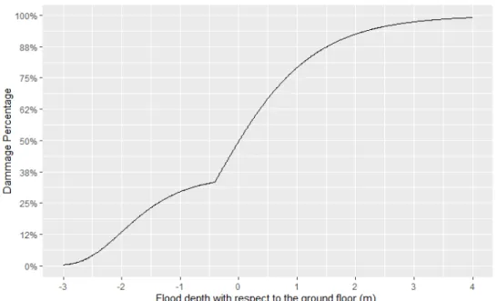
The damage caused by floods actually also depends on other factors than flood depth, like duration of flooding or water velocity. But, as stated by Bonnifait & Leclerc (2004), this information is difficult to consider, therefore, the predominant factor, flood depth, is usually taken into account. Figure 2.3 illustrates the damage curve used in this study, that corresponds to a one storey house with finished basement developed by Bonnifait & Leclerc (2004). It is important to mention that this curve considers only structural damages that refer to damages to the
building, i.e., it doesn’t considers content damages.
Figure 2.3 Damage Curve for One Storey House with Finished Basement Source: Data comes from Bonnifait & Leclerc (2004)
2.2 Data Transformation
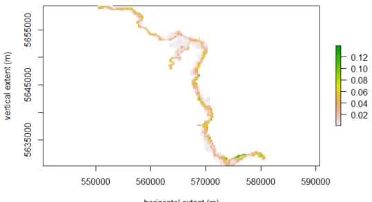
First, we calculate the flood depth in each pixel of the six floodplains according to the procedure explained in Appendix B. Then, we aggregate this information into one data set that contains the locations and the flood depths at each location. To calculate the flood losses, in percentages, we applied the damage curve, pre-viously mentioned, considering that hypothetical houses have basements of 2.2 metres of height. Now, we have a data set that contains the locations and flood losses at each location.
Then, assuming that each location has its own loss distribution, the flood aver-age losses at each location are calculated considering the percentiles of the loss
distribution.
The spatial distribution of the average loss in the study area is shown in Figure 2.4.
Figure 2.4 Expected Flood Loss (%) - 25-Meter Resolution
The information above will be used as input to apply clustering methods. For classical methods, the average loss in percentage will be used, and the location will allow us to view the spatial patterns. Whereas in spatial clustering methods, the location is included as an input in the model.
As is well-known, the size of the data plays an important role when running clustering methods. To handle large databases, as we have in this study, a common approach is to perform compression on the initial databases and then cluster the compressed data as stated by Han et al. (2001). Also, to avoid large spatial variations in nearby territories, it is more appropriate to enlarge the cluster unit measure.
Therefore, the information outlined above was compressed from 25-meter resolu-tion to 250-meter resoluresolu-tion, i.e., ten times larger cells, which will hereafter be the clustering unit measure. Figure 2.5 shows the spatial distribution of the av-erage loss in percentages with the lower resolution, which will be the input of the clustering methods.
Figure 2.5 Expected Flood Loss (%) - 250-Meter resolution
The standardization of features, that makes the variables centered with mean zero and scaled with standard deviation equals one, will be applied before entering the data in the clustering algorithms. This procedure will place equal weight on the variables when determining the clusters.
2.3 Applications
We have applied some classical and spatial clustering methods to define territories with similar flood risk profiles. Four clustering methods were applied twice; first,
only considering the loss due to flood, and, next, including the location, except for the SKATER clustering method, which already includes the location in its algorithm. For the algorithms that do not include the location to create groups, the spatial distribution of the results is used to visualize the clusters to see poten-tial natural patterns that homeowners might follow. Therefore, homeowners may be close together geographically but they are close given their exposition to flood risk.
For each clustering algorithm, two different approaches were used to select the number of groups. The first approach considers the optimum number of clus-ters with respect to the variance explained, and the second approach considers arbitrarily a fixed number of clusters equal to ten to compare all the algorithms under a standard approach. Therefore, we have fourteen different ways to group homeowners based on the flood risk to which they are exposed.
The optimal number of territories is selected considering the elbow plots of the variance explained by number of clusters. The variance explained is defined as the between-cluster variation divided by the total variance, and will always increase with number of clusters but will eventually slow down. Therefore, we select the number of clusters before the gain in variance explained starts to drop, as the optimal number. Therefore, a different optimal number of clusters is selected, depending on the clustering methods.
When comparing all clustering methods in Chapter 1, hereafter called statistical-based clustering methods, we can see in Figure 2.6 that K-means and Hybrid clustering methods based on flood loss have higher variance explained with each number of clusters. Although, the Hierarchical clustering method based only on flood loss tends to converge with K-means after ten clusters.
Figure 2.6 Elbow Plot of Statistical-Based Clustering Methods
homeowners most at risk faster because its approach is based on distances to create the hierarchical structure to differentiate groups. Moreover, given the hierarchical structure of the data, the Hierarchical method could be a good method to consider. On the other hand, the SKATER method, which has contiguous constraint, creates groups with larger variance of flood risk within groups that implies lower between-cluster dissimilarity compared with the other between-clustering methods.
Through the application of clustering methods, we have seen the trade-off be-tween flood loss similarity and location similarity. That is, when ratemaking territories are defined considering only similar flood loss, they are prone to set up non-contiguous territories. However, when ratemaking territories are created con-sidering contiguous bounds, clustering methods produce territories with a large variation in risk within territories. The complexity of the trade-off between flood
loss similarity and location similarity is an important aspect to consider when defining ratemaking territories.
We selected some relevant statistical-based clustering methods, specifically, K-means, Hierarchical, and SKATER methods, to study in more detail in the next sections. The Hybrid methods will not be detailed as we found that they gave similar results to K-means clustering. Hybrid and K-means methods, considering only losses and losses with location, have similar spatial distribution and distri-bution of clusters; and the lines that represent the variance explained of these methods by cluster numbers in Figure 2.6 are superposed. In fact, they are simi-lar methods because the Hybrid clustering method only considers the dendrogram to fix the initial centers and then follows the K-means algorithm. Therefore, we will not see these approaches any further in the following analyses. For more details, compare figures presented in this section against the ones presented in Appendix C. Specifically, compare Figures 2.7 and 2.8 against Figures C.3 and C.4, respectively, for clustering based on losses, and compare Figures 2.10 and 2.11 against Figures C.5 and C.6, respectively, for clustering based on losses and location.
2.3.1 K-Means Clustering
This algorithm is first applied to group homeowners based on flood losses. The K-means algorithm is run taking into account one to ten clusters to select the optimal number of clusters, considering fifty random initial configurations to assure that a local optimum has been reached. In Figure 2.6, we can see that the gain in variance explained drops after four clusters, so that number will be used as the optimal. Therefore, grouping homeowners into four clusters appropriately represents the data because they explain 91.79% of the data variance. Clustering homeowners
into ten groups explains 98.54% of the variance.
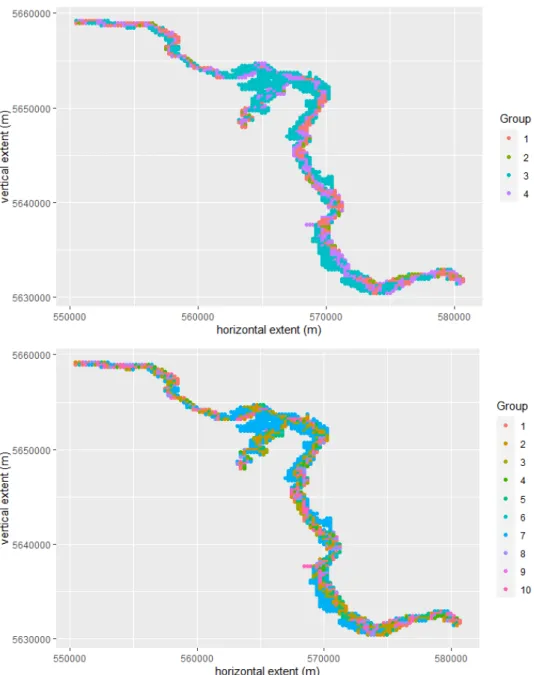
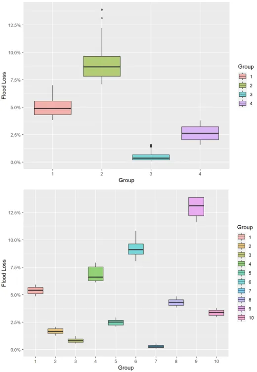
Figure 2.7 shows the spatial distributions of the groups in the study area, consid-ering four and ten clusters, where each color represents a group. Whereas Figure 2.8 shows the boxplots of each cluster, which are useful when comparing distri-butions between many groups. In addition, Table 2.1 shows the expected loss in percentage as well as the number of homeowners.
When the clustering process considers four groups, Group 3, which is the group that contains 51.1% of the total number of homeowners, is the least at risk as the expected flood loss is 0.49%, whereas Group 2 is the most at risk as their aggregate expected loss is 9.09%, the highest compared to the other groups. When considering ten groups of homeowners, the algorithm tries to find more differentiated groups. Under this procedure, it finds more riskier groups, e.g., Group 9 with an expected loss of 12.94%, and less riskier groups, like Group 7 with a 0.26% expected loss.
Importantly, the K-means clustering algorithm can help us to detect homeowners who are most at risk when compared to the mean of their groups. K-means cans also help us to detect the most at risk groups with small number of homeowners. For example, as in the case of Group 9, which is formed by only five homeowners who are most at risk.
When comparing the difference between the expected premium collected, which is paid by the homeowners based on its corresponding cluster, and the true ex-pected loss, based on the true distribution of losses in the pixel, the percentage of overpriced policyholders falls from 58% to 52% when the number of groups increases from 4 to 10. The distribution of these differences can be seen in Figure 2.9, where the second histogram, corresponding to the clustering with ten groups,
Figure 2.7 Spatial Distribution of Clusters Considering 4 and 10 Groups Based on Flood Losses - K-Means Algorithm
Figure 2.8 Boxplots of Clusters Considering 4 and 10 Groups Based on Flood Losses - K-Means Algorithm
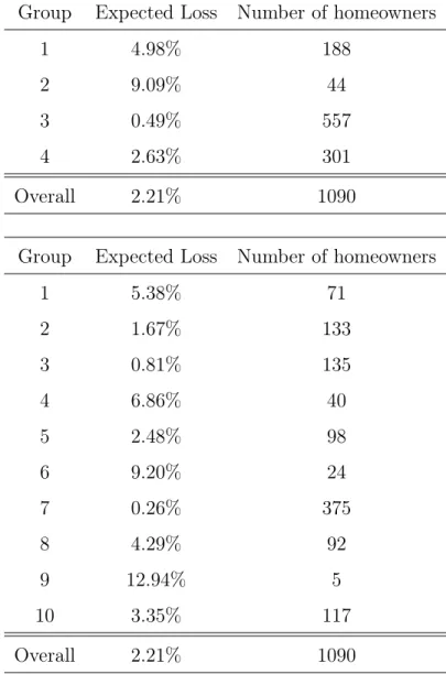
Table 2.1 Descriptive Statistics of Clusters Using K-Means Clustering Method Based on Flood Losses
Group Expected Loss Number of homeowners
1 4.98% 188
2 9.09% 44
3 0.49% 557
4 2.63% 301
Overall 2.21% 1090
Group Expected Loss Number of homeowners
1 5.38% 71 2 1.67% 133 3 0.81% 135 4 6.86% 40 5 2.48% 98 6 9.20% 24 7 0.26% 375 8 4.29% 92 9 12.94% 5 10 3.35% 117 Overall 2.21% 1090
Figure 2.9 Distribution of the Difference Between the Expected Premium Col-lected and the True Expected Loss for 4 (Top) and 10 (Bottom) Groups Based on Flood Losses - K-Means Algorithm
is more symmetric than the first one.
Next, this algorithm is applied to group homeowners based on flood losses and location. As in the first application of this algorithm, it was run considering one to ten clusters with fifty random initial configurations. The optimal number of clusters chosen is five, as the gain in variance explained drops after this point, as we can see in Figure 2.6.
Five groups explain 76.89% of data variance, while ten groups explain 88.32%. Therefore, the inclusion of the location in the algorithm makes the variance ex-plained decrease because the variation of risk within groups increases due to the trade off between flood loss similarity and location similarity. This leads to a larger spatial variation of risks grouped compared with the last clustering technique solely based on flood risk. To see a graphical explanation of this phenomenon, compare Figures 2.8 and 2.11.
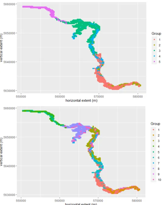
The spatial distribution of these arrangements are shown in Figure 2.10. We can see that the groups are more compacted than the clustering solely based on expected flood loss, although there is no contiguity in the groups. This non-contiguity characteristic can be seen, for example, in Group 2 and Group 4, on the five clustering arrangement, and in Group 9 and Group 10, in the ten cluster arrangement.
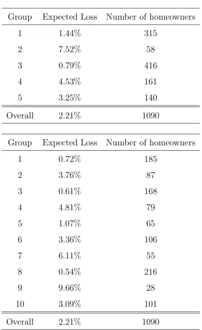
The expected loss in percentage for each group, as well as the number of homeown-ers classified in the groups, are shown in Table 2.2. Unlike the K-means clustering algorithm, based only on flood losses, this algorithm creates groups with a larger number of observations because it considers location in the grouping process. Figure 2.12 shows the distribution of the difference between the expected premium collected and the true expected loss. We can see that the distribution is more
Figure 2.10Spatial Distribution of Clusters Considering 5 and 10 Groups Based on Flood Losses and Location - K-Means Algorithm
Figure 2.11 Boxplots of Clusters Considering 5 and 10 Groups Based on Flood Losses and Location - K-Means Algorithm
Table 2.2 Descriptive Statistics of Clusters Using K-Means Clustering Method Based on Flood Losses and Location
Group Expected Loss Number of homeowners
1 1.44% 315 2 7.52% 58 3 0.79% 416 4 4.53% 161 5 3.25% 140 Overall 2.21% 1090
Group Expected Loss Number of homeowners
1 0.72% 185 2 3.76% 87 3 0.61% 168 4 4.81% 79 5 1.07% 65 6 3.36% 106 7 6.11% 55 8 0.54% 216 9 9.66% 28 10 3.09% 101 Overall 2.21% 1090
Figure 2.12 Distribution of the Difference Between the Expected Premium Col-lected and the True Expected Losses for 5 (Top) and 10 (Bottom) Groups Based on Flood Losses and Location - K-Means Algorithm
symmetric when more groups are considered. The same behavior was found in the clustering procedure based only on flood losses. Although, the percentage of overpriced policyholders increases from 58% to 60% when the number of groups increases from five to ten.
Comparing both clustering techniques, it is clear that K-means clustering based only on flood losses gives us the desired property of a low premium variation along with a better explanation of the data with four groups.
Also, even if no right answer is obtained from the clustering techniques, as they are exploratory tools to analyse data, henceforth when comparing models, we will use the K-means clustering method based only on flood losses.
2.3.2 Hierarchical Clustering
We have applied the Hierarchical clustering algorithm using a bottom-up ap-proach, also known as agglomerative, with complete linkage distance between clusters and Euclidean distances between observations.
This algorithm is applied first to group homeowners based on flood losses. As this method is based on distances, the structure of the data can be seen in Figure 2.13. This dendrogram illustrates the arrangement of the clusters. Each leaf of the dendrogram represents a homeowner, and as we move up the tree, more similar homeowners are merged. Then, the earlier the homeowners are fused the more similar they are to each other. Therefore, the homeowners that merge at the top of the tree will tend to be quite different. In fact, the height of the fusion tells us how different the observations or groups are.
We can see that if we cut the dendrogram at the height of 4, we obtain five clusters. This analysis can be complemented by analysing the variance explained by number
Figure 2.13 Dendrogram of Hierarchical Clustering Method Considering Flood Losses Using Complete Linkage
of clusters. In Figure 2.6, we can see that the gain in variance explained by the number of groups drops after three clusters to then increase when considering five clusters. Hence, we chose five groups as it gives a good representation of the data, 91.50% of variance explained, while ten groups explain 97.81% of the variance. The latter gives similar variance explained for the same number of groups using K-means clustering based only on flood losses.
Furthermore, we can see that the variance explained from Hierarchical methods does not increase smoothly in comparison to the K-means methods. This phe-nomenon occurs because K-means maximize the between-cluster variation when grouping observations, while hierarchical clustering creates groups based on dis-tances.
Figure 2.14 shows the spatial distribution of the homeowners. When the clustering process considers five groups, Group 1, which includes 59.44% of the homeowners, is the least at risk as the homeowners have an expected flood loss of 0.68%; whereas
Group 5 is the most at risk as the expected loss of the homeowners is 12.9%, the highest when compared to the other groups, as we can see in Table 2.3.
The clustering procedure considering ten groups has found three groups with a small number of homeowners, unlike K-means clustering that only found one small group. We can importantly conclude from this result that this procedure allows us to identify small groups of homeowners most at risk faster. In this particular case, Groups 8, 9, and 10 could be potential non-insurable homeowners. Con-sidering that this technique uses a hierarchical structure for group observations, non-insurable homeowners normally take longer to join other groups, as is the case for Groups 8, 9, and 10.
It is important to mention that this approach found the riskiest group when partitioning the data into five clusters, while K-means found the riskiest one when clustering the data in ten groups. Therefore, as we increased the number of groups in Hierarchical clustering, they found more differentiated groups.
With respect to the premium variation by group, it can be seen in Figure 2.15 that, as in the K-means clustering method based on flood losses, this clustering technique has low premium variation by group, which is a desirable property for ratemaking purposes.
Regarding the distribution of the difference between the expected premium col-lected and the true expected losses shown in Figure 2.16, we can see that clustering in five groups produces a skewed distribution to the left, while clustering in ten groups produced a less biased distribution. Specifically, the percentage of over-priced policyholders falls from 60% to 52%.
The Hierarchical technique was also applied to group homeowners based on flood losses and location. However, as with the K-means method based on flood losses
Figure 2.14Spatial Distribution of Clusters Considering 5 and 10 Groups Based on Flood Losses - Hierarchical Algorithm
Figure 2.15 Boxplots of Clusters Considering 5 and 10 Groups Based on Flood Losses - Hierarchical Algorithm
Table 2.3 Descriptive Statistics of Clusters Using Hierarchical clustering Based on Flood Losses
Group Expected Loss Number of homeowners
1 0.68% 648 2 3.11% 243 3 5.42% 170 4 9.21% 24 5 12.9% 5 Overall 2.21% 1090
Group Expected Loss Number of homeowners
1 1.48% 196 2 3.55% 133 3 4.97% 130 4 2.58% 110 5 0.33% 452 6 8.84% 18 7 6.86% 40 8 11.89% 2 9 10.28% 6 10 13.6% 3 Overall 2.21% 1090
Figure 2.16 Distribution of the Difference Between the Expected Premium Col-lected and the True Expected Losses for 5 (Top) and 10 (Bottom) Groups Based on Flood Losses - Hierarchical Algorithm