HAL Id: hal-00786055
https://hal.inria.fr/hal-00786055
Submitted on 12 Feb 2013
HAL is a multi-disciplinary open access
archive for the deposit and dissemination of
sci-entific research documents, whether they are
pub-lished or not. The documents may come from
L’archive ouverte pluridisciplinaire HAL, est
destinée au dépôt et à la diffusion de documents
scientifiques de niveau recherche, publiés ou non,
émanant des établissements d’enseignement et de
distributed-memory multifrontal solver
Jean-Yves l’Excellent, Mohamed W. Sid-Lakhdar
To cite this version:
Jean-Yves l’Excellent, Mohamed W. Sid-Lakhdar. Introduction of shared-memory parallelism in
a distributed-memory multifrontal solver. [Research Report] RR-8227, INRIA. 2013, pp.35.
�hal-00786055�
0249-6399 ISRN INRIA/RR--8227--FR+ENG
RESEARCH
REPORT
N° 8227
February 2013Introduction of
shared-memory
parallelism in a
distributed-memory
multifrontal solver
RESEARCH CENTRE GRENOBLE – RHÔNE-ALPES
Inovallée
655 avenue de l’Europe Montbonnot
a distributed-memory multifrontal solver
Jean-Yves L’Excellent
∗, Mohamed Sid-Lakhdar
†Project-Team ROMA
Research Report n° 8227 — February 2013 — 35 pages
Abstract: We study the adaptation of a parallel distributed-memory solver towards a shared-memory code, targeting multi-core architectures. The advantage of adapting the code over a new design is to fully benefit from its numerical kernels, range of functionalities and internal features. Although the studied code is a direct solver for sparse systems of linear equations, the approaches described in this paper are general and could be useful to a wide range of applications. We show how existing parallel algorithms can be adapted to an OpenMP environment while, at the same time, also relying on third-party optimized multithreaded libraries. We propose simple approaches to take advantage of NUMA architectures, and original optimizations to limit thread synchronization costs. For each point, the performance gains are analyzed in detail on test problems from various application areas.
Key-words: shared-memory, multi-core, NUMA, LU factorization, sparse matrix, multifrontal method
∗Inria, University of Lyon and LIP laboratory (UMR 5668 CNRS-ENS Lyon-INRIA-UCBL), Lyon, France
† ENS Lyon, University of Lyon and LIP laboratory (UMR 5668 CNRS-ENS Lyon-INRIA-UCBL), Lyon,
multifrontal `
a base de passage de messages
R´esum´e : Dans ce rapport, nous ´etudions l’adaptation d’un code parall`ele `a m´emoire dis-tribu´ee en un code visant les architectures `a m´emoire partag´ee de type multi-cœurs. L’int´erˆet d’adapter un code existant plutˆot que d’en concevoir un nouveau est de pouvoir b´en´eficier di-rectement de toute la richesse de ses fonctionnalit´es num´eriques ainsi que de ses caract´eristiques internes. Mˆeme si le code sur lequel porte l’´etude est un solveur direct multifrontale pour syst`emes lin´eaires creux, les algorithmes et techniques discut´es sont g´en´erales et peuvent s’appliquer `a des domaines d’application plus g´en´eraux. Nous montrons comment des algorithmes parall`eles exis-tant peuvent ˆetre adapt´es `a un environnement OpenMP tout en exploitant au mieux des librairies existantes optimis´ees. Nous pr´esentons des approches simples pour tirer parti des sp´ecificit´es des architectures NUMA, ainsi que des optimisations originales permettant de limiter les coˆuts de synchronisation dans le mod`ele fork-join que l’on utilise. Pour chacun de ces points, les gains en performance sont analys´es sur des cas tests provenant de domaines d’applications vari´es. Mots-cl´es : m´emoire partag´ee, multi-cœur, NUMA factorisation LU, m´ethode multifrontale, matrice creuse
Contents
1 Introduction 3
2 Context of the study 5
2.1 Multifrontal method and solver . . . 5
2.2 Experimental environment . . . 6
3 Multithreaded node parallelism 9 3.1 Use of multithreaded libraries . . . 9
3.2 Directives-based loop parallelism . . . 9
3.3 Experiments on a multi-core architecture . . . 10
4 Introduction of multithreaded tree parallelism 11 4.1 Balancing work among threads (AlgFlops algorithm) . . . 12
4.2 Minimizing the global time (AlgTime algorithm) . . . 13
4.2.1 Performance model . . . 14
4.2.2 Simulation . . . 16
4.3 Implementation . . . 17
4.4 Experiments . . . 18
5 Memory affinity issues on NUMA architectures 20 5.1 Performance of dense factorization kernels and NUMA effects . . . 20
5.1.1 Machine load . . . 20
5.1.2 Memory locality and memory interleaving . . . 22
5.2 Application to sparse matrix factorizations . . . 23
5.3 Performance analysis . . . 23
5.3.1 Effects of the interleave policy . . . 23
5.3.2 Effects of modifying the performance models . . . 26
6 Recycling idle cores 26 6.1 Core idea and algorithm . . . 27
6.2 Analysis and discussion . . . 29
6.3 Early idle core detection and NUMA environments . . . 30
6.4 Sensitivity to Lth height . . . 31
7 Conclusion 32
1
Introduction
Since the arrival of multi-core systems, many efforts must be done to adapt existing software in order to take advantage of these new architectures. Whereas shared-memory machines were common before the mid-90’s, since then, message-passing (and in particular MPI [13]) has been widely used to address distributed-memory clusters with large numbers of nodes. Although message-passing can be applied inside multi-core processors, the shared-memory paradigm is also a convenient way to program them. Unfortunately, codes that were designed a long time ago for SMP machines often do not exhibit good performance on today’s multi-core architectures. The costs of synchronizations, the increasing gap between processor and memory speeds, the NUMA (Non-Uniform Memory Accesses) effects and the increasing complexity of modern cache hierarchies are among the main difficulties encountered.
In this study, we are interested in a parallel direct approach for the solution of sparse systems of linear equations of the form
Ax = b, (1) where A is a sparse matrix, b is the right-hand side vector (or matrix) and x is the unknown vector. Several parallel direct solvers, based on matrix factorizations and targeting distributed-memory computers have been developed over the years [18, 27, 19]. In our case, we consider that matrix A is unsymmetric but has a symmetric pattern, at the possible cost of adding explicit zeros when treating matrices with an unsymmetric pattern. We rely on the multifrontal method [15] to decompose A under the form A = LU . In this approach, the task graph is a tree called elimination tree, which must be processed from the leaves to the root following a topological order (i.e., children must be processed before their parent). At each node of the tree, a partial factorization of a small dense matrix is performed; nodes on distinct subtrees can be processed independently. Because sparse direct solvers using message-passing often have a long development cycle, sometimes with many functionalities and numerical features added over the years, it is not always feasible to redesign them from scratch, even when computer architectures evolve a lot.
The objective of this paper is thus to study how, starting from an existing parallel solver using MPI, it is possible to adapt it and improve its performance on multi-core architectures. Although the resulting code is able to run on hybrid-memory architectures, we consider here a pure shared-memory environment. We use the example of the MUMPS solver [3, 5], but the methodology and approaches described in this paper are more general. We study and combine the use (i) of multithreaded libraries (in particular BLAS– Basic Linear Algebra Subprograms [25]); (ii) of loop-based fine grain parallelism based on OpenMP [1] directives; and (iii) of coarse grain OpenMP parallelism between independent tasks. On NUMA architectures, we show that the memory allocation policy and resulting memory affinity has a strong impact on performance and should be chosen with care, depending on the set of threads working on each task. Furthermore, when treating independent tasks in a multithreaded environment, if no ready task is available, a thread that has finished its share of the work will wait for the other threads to finish and become idle. In an OpenMP environment, we show how, technically, it is in that case possible to re-assign idle threads to active tasks, increasing dynamically the amount of parallelism exploited and speeding up the corresponding computations.
In relation to this work, we note that multithreaded sparse direct solvers aiming at addressing multi-core machines have been the object of a lot of work [2, 7, 10, 12, 16, 23, 18, 22, 26, 33]. Our approach and contribution in this paper are different in several aspects. First, we start from an existing code, originally designed for distributed-memory architectures, with a wide range of specific functionalities and numerical features; our objective is to show how such a code can be modified without a strong redesign. Second, most solvers use serial BLAS libraries and manage all the parallelism themselves; on the contrary, we aim at taking advantage as much as possible of existing multithreaded BLAS libraries, that have been the object of a lot of tuning by specialists of dense linear algebra. Notice that in the so called DAG-based approaches [10, 21] (and in the code described in reference [2], much earlier), tree parallelism and node parallelism are not separated: each individual task can be either a node in the tree or a subtask inside a frontal matrix. This is also the case of the distributed-memory approach we start from, where a processor can for example start working on a parent node even when some work remains to be done at the child level [4]. In our case and in order to keep the management of threads simple, we study and push as far as possible the approach consisting in using tree parallelism up to a certain level, and then switching to node parallelism in a radical manner, at the cost of an acceptable synchronization. Some recent evolutions in dense linear algebra tend to use task dispatch engines [10, 21] or runtime systems like Dague [8] or StarPU [6], for example. Such
approaches start to be experimented in the context of sparse direct solvers. In particular, the Pastix [19] solver has an option to use such runtime systems, with the advantage of being able to use not only multi-core systems but also accelerators. However, numerical pivoting issues leading to dynamic task graphs, or specific numerical features not available in dense libraries relying on runtime systems, or application-specific approaches to scheduling, still make it hard to use such runtime systems in all cases. Remark that, even if we were using such runtime systems instead of OpenMP, most of the observations and contributions of this paper would still apply.
The paper is organized as follows. In Section 2, we present the multifrontal approach used and the software we rely on, together with our experimental setup. In Section 3, we assess the limits of the fork-join approach to multithreaded parallelism, when using multithreaded BLAS libraries and OpenMP directives. We also compare such an approach to the use of MPI and to different combinations of MPI processes and threads. After Section 3, we focus on a pure shared-memory environment, where only one MPI process is used. In Section 4, we propose and study an algorithm to go further in the parallelization thanks to a better granularity of parallelism in the part of our task graph (the elimination tree) where this is necessary. In Section 5, the case of NUMA architectures is studied, where we show how the memory accesses can dramatically impact performance. In Section 6, because the approach retained involves a synchronization when switching from one type of parallelism to the other, we study how OpenMP allows to reuse idle cores by assigning them to active tasks dynamically. Finally, we conclude by summarizing the lessons learned while adapting an existing code to multi-core architectures, and we give some perspectives to this work.
2
Context of the study
2.1
Multifrontal method and solver
We refer the reader to [15, 29] for an overview of the multifrontal method. In this section, we only provide the algorithmic details of our multifrontal solver that will be necessary in the next sections.
As said in the introduction, the task graph in the multifrontal method is a tree called
elim-ination tree. At each node of this tree, a dense matrix called front or frontal matrix is first
assembled, using contributions from its children and entries of the original matrix; some of its variables are then factorized (partial factorization), and the resulting Schur complement formed (updated but not yet factorized block) is copied for future use. The Schur complement is also called contribution block, because it will contribute to the assembly of the parent’s frontal matrix. At the root node, a full factorization is performed.
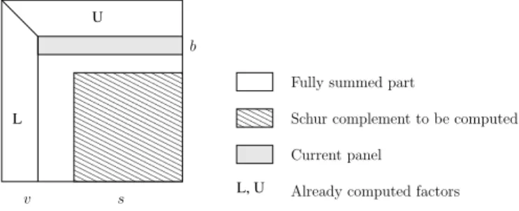
The three steps above namely assembly, factorization and stacking, correspond to three com-putational kernels of our multifrontal solver, which we describe in Algorithms 1, 2, and 3. When assembling contributions in the frontal matrix of a parent (Algorithm 1), indirections are required because contiguous variables in the contribution block of a child are not necessarily contiguous in the parent. The corresponding summation is called an extend-add operation. Rows and columns in the parent that have received all their contributions are said to be fully summed. The method places them first in the front, as shown in Figure 1, and the corresponding variables can be factorized, as shown in Algorithm 2. In the factorization, the fully summed rows are factorized panel by panel, then the other rows are updated using BLAS calls of large size. Finally, the stacking operation consists in saving the Schur complement in a stack area, for future use as a contribution block at the parent level. We note that the memory accesses for contribution blocks follow a stack mechanism as long as nodes are processed using a postorder. Furthermore, in our software environment, a work array is preallocated, in which factors are stored on the
left, contribution blocks are stored on the right, and current frontal matrices are stored right on top of the factors area. This work array is typical in multifrontal codes as it allows for more control and optimizations in the memory management than dynamic allocation. Because frontal matrices are stored by rows, only the non fully summed rows of the L factors must be moved at line 5 of Algorithm 3. At that line, in the case of an out-of-core setting where factors have been written to disk panel by panel (or in the case they are not needed), factors are simply discarded.
0000000 0000000 0000000 0000000 0000000 0000000 0000000 0000000 0000000 0000000 0000000 0000000 1111111 1111111 1111111 1111111 1111111 1111111 1111111 1111111 1111111 1111111 1111111 1111111 00 00 00 11 11 11 L, U L U v s b
Already computed factors Current panel
Schur complement to be computed Fully summed part
Figure 1: Structure of a frontal matrix.
Algorithm 1 Sketch of the assembly of a set of children into a parent node N .
1: 1. Build row and column structures of frontal matrix associated to nodeN :
2: Merge lists of variables from children and from original matrix entries to be assembled in N
3: Build indirections (overwriting index list IN Dc of child c with the relative positions in the
parent)
4: 2. Numerical assembly:
5: for all children c of node N do
6: for all contribution rows i of child c do 7: for all contribution columns j of child c do
8: Assemble entry (i,j) at position (IN Dc(i), IN Dc(j)) of parent (extend-add operation)
9: end for
10: end for
11: Assemble entries from original matrix in fully summed rows and columns of N
12: end for
There are typically two sources of parallelism in multifrontal methods. From a coarse-grain point of view, elimination trees are DAGs that define dependencies between their fronts. The structure of tree then offers an inner parallelism, which consists in factorizing different indepen-dent fronts at the same time. This is tree parallelism. From a fine-grain point of view, the partial factorization of a frontal matrix at a given node of the elimination tree (see Algorithm 2) can also be parallelized: this is called node parallelism. In a distributed-memory environment, the MUMPS solver we use to illustrate this study implements these two types of parallelism, which were called type 1 and type 2 parallelism [4], respectively. Tree parallelism decreases near the root, where node parallelism generally increases because frontal matrices tend to be bigger.
2.2
Experimental environment
The set of test problems used in our experiments is given in Table 1. Although some matrices are symmetric, we only consider the unsymmetric version of the solver. We use a nested dissection ordering (in our case, METIS [24]) to reorder the matrices. By default, we use double precision
Algorithm 2 BLAS calls during partial dense factorization of a frontal matrix F of order v + s with v variables to eliminate and a Schur of order s. b is the block size for panels. We assume that all pivots are eliminated.
1: for all horizontal panels P = F (k : k + b − 1, k : v + s) in fully summed block do
2: BLAS 2factorization of the panel:
3: while A stable pivot can be found in columns k : v of P do
4: Perform the associated row and/or column exchanges
5: Scale pivot column in panel ( SCAL) 6: Update panel ( GER)
7: end while
8: Update fully summed column block F (k + b : v, k : k + b − 1) ( TRSM)
9: Right-looking update of remaining fully summed part F (k + b : v, k + b : v + s) ( GEMM)
10: end for
11: % All fully summed rows have been factorized
12: Update F (v + 1 : v + s, 1 : v) ( TRSM)
13: Update Schur complement F (v + 1 : v + s, v + 1 : v + s) ( GEMM)
Algorithm 3 Stacking operation for a frontal matrix F of order v + s. Frontal matrices are stored by rows.
1: Reserve space in stack area
2: for i = v + 1 to v + s do
3: Copy F (i, v + 1 : v + s) to stack area
4: end for
arithmetic, real or complex. The horizontal lines in the table define five areas; the first one (at the top) corresponds to matrices for which there are very large fronts (e.g. 3D problems). The third one corresponds to matrices with many small fronts, including sometimes near the root (e.g. circuit simulation matrices). The second one corresponds to matrices intermediate between those two extremes. Finally, the fourth (resp. fifth) zone corresponds to 3D (resp. 2D) geophysics applications.
Matrix Symmetry Arithmetic N N Z Application field 3Dspectralwave Sym. real 680943 30290827 Materials AUDI Sym. real 943695 77651847 Structural conv3D64(*) Uns. real 836550 12548250 Fluid Serena(*) Sym. real 1391349 64131971 Structural sparsine Sym. real 50000 1548988 Structural
ultrasound Uns. real 531441 33076161 Magneto-Hydro-Dynamics dielFilterV3real Sym. real 1102824 89306020 Electromagnetism
Haltere Sym. complex 1288825 10476775 Electromagnetism ecl32 Uns. real 51993 380415 Semiconductor device G3 circuit Sym. real 1585478 7660826 Circuit simulation QIMONDA07 Uns. real 8613291 66900289 Circuit simulation GeoAzur 3D 32 32 32 Uns. complex 110592 2863288 Geo-Physics GeoAzur 3D 48 48 48 Uns. complex 262144 6859000 Geo-Physics GeoAzur 3D 64 64 64 Uns. complex 512000 13481272 Geo-Physics GeoAzur 2D 512 512 Uns. complex 278784 2502724 Geo-Physics GeoAzur 2D 1024 1024 Uns. complex 1081600 9721924 Geo-Physics GeoAzur 2D 2048 2048 Uns. complex 4260096 38316100 Geo-Physics Table 1: Set of test problems. N is the order of the matrix and N Z its number of nonzero ele-ments. The matrices come from Tim Davis’ collection (University of Florida), from the GridTLSE collection (University of Toulouse) and from geophysics applications [30, 34]. “Sym.” is for sym-metric matrices and “Uns.” for unsymsym-metric matrices. For symsym-metric matrices, we work on the unsymmetric problem associated, although the value of N Z reported only represents the number of nonzeros in the lower triangle. The largest matrices, indicated by “(*)”, will only be used on the largest machine, dude.
In our study, we rely on the two multi-core based computers below: • hidalgo:
– Processor: 2 × 4-Core Intel Xeon Processor E5520 2.27 GHz (Nehalem). – Memory: 16 GigaBytes.
– Compiler: Intel compilers (icc and ifort) version 12.0.4 20110427. – BLAS: Intel(R) Math Kernel Library (MKL) version 10.3 update 4. – Location: ENSEEIHT-IRIT, Toulouse.
• dude:
– Processor: 4 × 6-Core AMD Opteron Processor 8431 2.40 GHz (Istanbul). – Memory: 72 GigaBytes.
– BLAS: Intel(R) Math Kernel Library (MKL) version 10.3 update 4.
In one of the experiments, we also use a symmetric multiprocessor without NUMA effects from IDRIS1
: • vargas:
– Processor: 32-Core IBM Power6 Processor 4.70 GHz. – Memory: 128 GigaBytes.
– Compiler: xlf version 13.1 and xlc version 11.1. – BLAS: ESSL version 3.3.
3
Multithreaded node parallelism
In this section, we describe sources of multithreaded parallelism inside each computational task: multithreaded libraries and insertion of OpenMP directives. The combination of this type of shared-memory parallelism with distributed-memory parallelism is also discussed in Section 3.3.
3.1
Use of multithreaded libraries
The largest part of the multifrontal factorization time is spent in dense linear algebra kernels, namely, the BLAS library. Therefore, reducing the corresponding time is the first source of improvement. A straightforward way to do this consists in using existing optimized multithreaded BLAS libraries. This is completely transparent to the application in the sense that only the link phase is concerned, requiring no change to the algorithms, nor to the code.
In our case, the largest amount of computation is spent in the GEMM and TRSM calls from Algorithm 2. Because the update on F21 and F22 are done only after the fully-summed block is
factorized (lines 12 and 13), the corresponding TRSM and GEMM operations operate on very large matrices, on which multithreaded BLAS libraries have freedom to organize the computations using an efficient parallelization.
Several optimized BLAS libraries exist, for example ATLAS [35], OpenBLAS, MKL (from Intel), ACML (from AMD), or ESSL (from IBM). As said in Section 2.2, we use MKL. One difficulty with Atlas is that the number of threads has to be defined at compile-time, and one difficulty we had with OpenBLAS (formerly GotoBLAS) was its interaction with OpenMP regions [11]. With the MKLversion used, the MKL DYNAMIC setting (similar to OMP DYNAMIC) is activated by default, so that providing too many threads on small matrices does not result in speed-downs: extra threads are not used. This was not the case with some earlier versions of MKL, where it was necessary to manually set the number of threads to 1 (thanks to the OpenMP routine omp set num threads) for fronts too small to benefit from threaded BLAS. Unless stated otherwise, the experiments reported are with MKL DYNAMIC set to its default (true) value.
3.2
Directives-based loop parallelism
Loops can easily be parallelized in assembly and stack operations, as was initiated in [11]. Pivot search operations can also be multithreaded. The main difficulties encountered consisted in choosing, for each loop, the minimum granularity above which it was worth parallelizing it.
Concerning the assembly operations (Algorithm 1), the simplest way of parallelizing them consists in using a parallel OpenMP loop at line 6 of the algorithm. This way, all rows of a given
child are assembled in parallel. We observed experimentally that such a parallelization is only worth doing when the order of the contribution block to be assembled from the child is bigger than 300. Another approach to parallelize Algorithm 1, that would lead to a slightly larger granularity, would consist in splitting the rows of the parent node in a number of zones that would be assembled in parallel, where each zone sees all needed contribution rows assembled in it (from all children). Such an approach is used in the distributed version of our solver. In case of multithreading, it has not been experimented, although it might be interesting for wide trees in cases where the assembly costs may be large enough to compensate for the additional associated symbolic costs.
Stack operations (Algorithm 3), which are basically memory copy operations, can also be parallelized by using a parallel loop at line 2 of the algorithm. Again, a minimum granularity has to be ensured in order to avoid speed-downs on small fronts.
We use the default scheduling policy for OpenMP, which, in our environments, consists in using static chunks of maximum size. The larger the frontal matrices, the larger the gains obtained on assembly and stack operations.
3.3
Experiments on a multi-core architecture
In Table 2, we report the effects of using threaded BLAS and OpenMP directives on the factorization time on 8 cores of hidalgo; we also compare these results with an MPI parallelization using MUMPS 4.10.0, with different combinations of threads per process for a total of 8 cores. In case of multiple threads per MPI process, threaded BLAS and OpenMP directives are used within each MPI process, in such a way that the total number of threads is 8.
On the first set of matrices (3Dspectralwave, AUDI, sparsine, ultrasound80), the ratio of large fronts over small fronts in the associated elimination tree is high. Hence, the more threads per MPI process, the best the performance, because node parallelism and the underlying multithreaded BLAS routines can reach their full potential on many fronts. On the second set of matrices, the ratio of large fronts over small fronts is medium; the best computation times are generally reached when mixing tree parallelism at the MPI level with node parallelism at the BLASlevel. On the third set of matrices, where the ratio of large fronts over small fronts is very small (most fronts are small), using only one core per MPI process is often the best solution: tree parallelism is critical whereas node parallelism does not bring any gain. This is because parallel BLASis not efficient on small fronts where there is not enough work for all the threads. On the Geoazurseries of matrices, we also observe that tree parallelism is more critical on 2D problems than on 3D problems: on 2D problems, the best results are obtained with more MPI processes (and less threads per MPI process).
We observe that OpenMP directives improve in general the amount of node parallelism (com-pare columns “Threaded BLAS” and “Threaded BLAS + OpenMP directives” in the “1 MPI × 8 threads” configuration), but that the gains are limited. With the increasing number of cores per machine, this approach is only scalable when most of the work is done in very large fronts (e.g., on very large 3D problems). Otherwise, tree parallelism is necessary. The fact that message-passing in our solver was primarily designed to tackle parallelism between computer nodes rather than inside multi-core processors, and the availability of high performance multithreaded BLAS libraries lead us to think that both node and tree parallelism should be exploited at the shared-memory level. The path we follow in the next section thus consists in introducing multithreaded tree parallelism.
Sequential threaded threaded BLAS + Pure MPI BLAS only OpenMPdirectives
1 MPI × 1 MPI × 1 MPI × 2 MPI × 4 MPI × 8 MPI × Matrix 1 thread 8 threads 8 threads 4 threads 2 threads 1 thread 3Dspectralwave 2061.95 372.83 371.87 392.98 387.57 N/A AUDI 1270.20 251.14 249.21 250.87 300.43 315.85 sparsine 314.58 62.52 61.87 82.01 80.22 94.42 ultrasound80 441.84 89.05 89.16 95.67 124.07 124.10 dielFilterV3real 271.96 60.69 59.31 52.13 47.85 61.92 Haltere 691.72 121.29 120.81 115.18 140.34 145.55 ecl32 3.00 1.13 1.05 0.93 0.98 0.94 G3 circuit 16.99 8.84 8.73 6.24 4.21 3.61 QIMONDA07 25.78 27.42 28.49 18.21 9.63 5.54 GeoAzur 3D 32 32 32 75.74 16.09 15.84 16.28 18.68 19.62 GeoAzur 3D 48 48 48 410.78 73.90 72.96 69.71 95.02 106.86 GeoAzur 3D 64 64 64 1563.01 254.47 254.38 276.98 303.15 360.96 GeoAzur 2D 512 512 4.48 2.30 2.33 1.46 1.40 1.56 GeoAzur 2D 1024 1024 30.97 11.54 11.65 8.38 6.53 6.21 GeoAzur 2D 2048 2048 227.08 64.41 64.27 49.97 43.33 43.44 Table 2: Factorization times (seconds) on hidalgo, with different core-process configurations. Times are in seconds. N/A: the factorization ran out of memory. For each matrix, the best time obtained appears in bold.
4
Introduction of multithreaded tree parallelism
We now want to overcome the limitations of the previous approach, where we have observed limited gains from node parallelism on small frontal matrices. Even when there are large frontal matrices near the top of the tree, node parallelism may be insufficient in the bottom of the tree, where tree parallelism could be exploited instead. The objective of this section is thus to introduce tree parallelism at the threads level, allowing different frontal matrices to be treated by different threads. Many algorithms exist to exploit tree parallelism in sparse direct methods. Among them, the proportional mapping [32] and the Geist-Ng algorithm [17] have been widely used. They have for example inspired the mapping algorithms of MUMPS in distributed-memory environments. The Geist-Ng algorithm had been originally designed for shared-memory multiprocessor environments for parallel sparse Cholesky factorizations. Then, it has been adapted to distributed-memory environments and to other kinds of sparse factorizations. Its goal is to “achieve load balancing
and a high degree of concurrency among the processors while reducing the amount of processor-to-processor data communication”[17]. For this, tree parallelism is exploited. Since the time of the
development of this algorithm, multiprocessor architectures have evolved a lot, containing more and more cores, and new caches have appeared with increasing structure complexity. Therefore, we base our work on the Geist-Ng algorithm, trying to adapt it accordingly.
Sections 4.1 and 4.2 present two variants of the Geist-Ng algorithm, aiming at determining a layer in the tree under which only tree parallelism is used. This layer will be referred to as Lth. In Section 4.3, we then explain how our existing multifrontal solver can be modified to
take advantage of tree parallelism, without a deep redesign. We finally show in Section 4.4 some experimental results obtained with our variants of the Geist-Ng algorithm (Lthbased algorithms)
4.1
Balancing work among threads (AlgFlops algorithm)
The AlgFlops algorithm is essentially based on the Geist-Ng algorithm, whose main idea is
”Given an arbitrary tree and P processors, to find the smallest set of branches in the tree such that this set can be partitioned into exactly P subsets, all of which require approximately the same amount of work . . . ”[17].
Geist and Ng proceed in two distinct steps: (a) find a layer separating the bottom from the top of the tree (which we call Lth); and (b) factorizing the elimination tree. The goal of the layer
is to identify a set of branches in the bottom of the tree that can be mapped onto the processors with an acceptable load balance. The remaining nodes, above Lth, are then assigned to all the
processors in a round-robin manner.
In order to find Lth, the algorithm starts by defining it as the root of the tree. (In case of
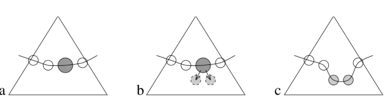
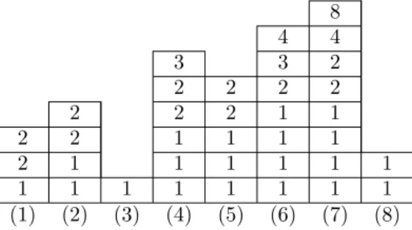
a forest, the initial layer contains the roots of all forest’s trees.) As shown in Algorithm 4 and Figure 2, the iterative procedure replaces the largest subtrees by their children until finding a satisfactory layer. More precisely, the first phase consists in identifying the heaviest subtree and substituting its root with the roots of its children. Because of the dependencies between a parent node and its children, expressed by the elimination tree, the algorithm must respect the property that if a node is on Lth, none of its ancestors can belong to this layer. The second phase consists
in mapping the independent subtrees from the Lth layer on the processors. The third phase
consists in checking whether the current layer respects a certain acceptance criterion, based on load balance. If this criterion is met, the algorithm then terminates. Algorithm 4 depends on the following points:
• Subtree cost: The cost of a subtree is here defined as the sum of the floating-point operations needed to work on the fronts that constitute it.
• Subtree mapping: The problem of mapping subtrees over processors is known as the multiprocessor scheduling problem. It is an NP-complete optimization problem which can be efficiently solved by the LPT (Longest Processing Time first) algorithm. The maximal runtime ratio between LPT and the optimal algorithm has been proved to be 4/3 - 1/(3p), where p is the number of processors [14].
• Acceptance criterion: The acceptance criterion is a user-defined tolerance corresponding to the minimal load balance of the processors under Lth (when the subtrees are mapped
on the processors with LPT).
Algorithm 4 Geist-Ng analysis step: finding a satisfactory layer Lth.
Lth← roots of the elimination tree
repeat
Find the node N in Lth, whose subtree has the highest estimated cost {Subtree cost}
Lth← Lth∪ {children of N } \ {N }
Map Lth subtrees onto the processors {Subtree mapping}
Estimate load balance:load(least-loaded processor)
load(most-loaded processor)
until load balance > threshold {Acceptance criterion}
Concerning the numerical factorization, each thread picks the heaviest untreated subtree under Lth and factorizes it. If no more subtrees remain, the thread goes idle and waits for the
others to finish. Then, whereas the Geist-Ng algorithm only used tree parallelism, our proposed AlgFlopsalgorithm uses tree parallelism under Lth but also node parallelism above it, for the
c
b
a
Figure 2: One step in the construction of the layer Lth.
following reasons: (i) there are fewer nodes near the root of a tree, and more nodes near the leaves; (ii) fronts near the root often tend to be large, whereas fronts near the leaves tend to be small; (iii) this approach matches the pros and cons of each kind of parallelism observed in Section 3.3.
This approach still has a few limitations. First, the acceptance criterion threshold may need to be tuned manually, and may depend on the test problem and target computer. We observed that a threshold of 90% is an adequate default parameter for most problems, especially when reordering is performed with nested dissection-based techniques such as Metis [24] or Scotch [31]. However, with some matrices, it is not always possible to reach a too high threshold. In such cases, unless another arbitrary stopping criterion is used, the algorithm will show a poor performance as it may not stop until the Lth layer contains all the leaves of the elimination
tree. Not only the determination of Lth will be costly but also the resulting Lth layer could be
unadapted. Second, the 90% criterion is based on a flops metric for the subtrees and we often observe in practice a balance worse than 90% in terms of runtime under Lth. This is due to the
fact that the number of floating-point operations is not an accurate measure of the runtime on modern architectures with complex memory hierarchies: typically, the Gflops/s rate will be much bigger for large frontal matrices than for small ones. This limitation is amplified on unbalanced trees because the ratio of large vs. small frontal matrices may then be unbalanced over the subtrees. Third, and more fundamentally, a good load balance under Lth may not necessarily
lead to an optimal total run time (sum of the run times under and above Lth).
4.2
Minimizing the global time (AlgTime algorithm)
To overcome the aforementioned limitations, we propose a modification of the AlgFlops algo-rithm, which we refer to as AlgTime. This new version modifies the computation of Lth, while
the factorization step remains unchanged, with tree parallelism underLth and node parallelism
above Lth.
One main characteristic of the AlgTime algorithm is that, instead of considering the number of floating-point operations, it focuses on the total runtime. Furthermore, the goal is not to achieve a good load balance but rather to minimize the total factorization time. It relies for that on a performance model of the mono-threaded (under Lth) and multi-threaded (above
Lth) processing times, estimated on dense frontal matrices, as will be explained below (see
Section 4.2.1). Thanks to this model, it becomes possible to get an estimate of the cost associated to a node both under and above Lth, where mono-threaded and multi-threaded dense kernels
are, respectively, applied.
The AlgTime algorithm (see Algorithm 5) computes layer Lth using the same main loop
as in the Geist-Ng algorithm. However, at each step of the loop, it keeps track of the total factorization time induced by the current Lth layer as the sum of the estimated time that will
be spent under and above it. Hence, as long as the estimated total time decreases, we consider that the acceptance criterion has not been reached yet. Simulations showed, however, that this method can fail reaching the global minimum because the algorithm may be trapped in a local minimum.
In order to get out of local minima, the algorithm proceeds as follows. Once a (possibly local) minimum is found, the current Lth is temporarily saved as the optimal Lth found so far but the
algorithm continues for a few extra iterations. The maximum number of additional iterations (called extra iterations) is a user-defined parameter. The algorithm stops if no further decrease in time is observed within the authorized extra iterations. Otherwise, the algorithm continues after reseting the counter of additional iterations each time a layer better than all previous ones is reached. We observed that a value of 100 extra iterations is largely enough to reach the global minimum on all problems tested, without inducing any significant extra cost. By nature, this algorithm is meant to be robust against any shape of elimination tree, and is meant to be robust among Lth-like algorithms. In particular, on unbalanced trees with large leaves, the algorithm
is allowed to choose an Lth below some of the leaves (or below all leaves, in which case Lth is
empty and the algorithm stops). Algorithm 5 AlgTime algorithm.
Lth← roots of the assembly tree
Lth best ← Lth best total time ← ∞ new total time ← ∞ cpt ← extra iterations
repeat
Find the node N in Lth, whose subtree has the highest estimated serial time
Lth← Lth∪ {children of N } \ {N }
Map Lth subtrees onto the processors
Simulate time under Lth
time above Lth← time above Lth+ cost(N , nbthreads) new total time ← time under Lth+ time above Lth
if new total time < best total time then Lth best ← Lth
best total time ← new total time cpt ← extra iterations else cpt ← cpt − 1 end if until cpt = 0 or Lth is empty Lth← Lth best 4.2.1 Performance model
Let α be the GFlops/s rate of the dense factorization kernel described in Algorithm 2, which is responsible of the largest part of the execution time of our solver. α depends on the number v of eliminated variables and on the size s of the computed Schur complement. We may think of modeling the performance of dense factorization kernels by representing α under the form of a simple analytical formula parametrized experimentally. However, due to the great unpredictabil-ity of both hardware and software, it is difficult to find an accurate-enough formula. For this
reason, we have run a benchmarking campaign on dense factorization kernels on a large sample of well-chosen dense matrices for different numbers of cores. Then, using interpolation, we have obtained an empirical grid model of performance. Note that an approach based on performance models of BLAS routines has already been used in the context of the sparse solver PaStiX [20].
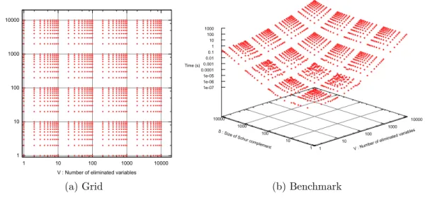
Given a two-dimensional field associated to v and s, we define a grid whose intersections represent the samples of the dense factorization kernel’s performance benchmark. This grid must not be uniform. Indeed, α tends to vary greatly for small values of v and s, and tends to have a constant asymptotic behavior for large values. This is directly linked to the BLAS effects. Consequently, many samples must be chosen on the region with small v and s, whereas less and less samples are needed for large values of these variables. An exponential grid might be appropriate. However, not enough samples would be kept for large values of v and s. That is why we have adopted the following linear-exponential grid, melting linear samples on some regions, whose step grows exponentially between the regions:
v or s ∈ [1, 10] step = 1 v or s ∈ [10, 100] step = 10 v or s ∈ [100, 1000] step = 100 v or s ∈ [1000, 10000] step = 1000
Figure 4.2.1 (a) shows this grid in log-scale and Figure 4.2.1 (b) shows the benchmark on one core on hidalgo. In order to give an idea of the performance of the dense factorization kernels
1 10 100 1000 10000 1 10 100 1000 10000 S : S ize o f S ch ur co m pl em en t
V : Number of eliminated variables
(a) Grid 1 10 100 1000 10000 1 10 100 1000 10000 1e-07 1e-06 1e-05 0.00010.001 0.01 0.11 10 100 1000 Time (s) V : Number of eliminat ed variable s S : Size of Schur co mplement (b) Benchmark Figure 3: Grid and benchmark on one core of hidalgo.
based on Algorithm 2, the GFlop/s rate of the partial factorization of a 4000 × 4000 matrix, with 1000 eliminated pivots, is 9.42GF lops/s on one core, and is 56.00GF lops/s on eight cores (a speed-up of 5.95). We note that working on the optimization of dense kernels is outside the scope of this paper.
for any arbitrary desired point (v,s) using the following simple bilinear interpolation: α(v, s, N bCore) ≈ α(v1, s1, N bCore) (v2− v1)(s2− s1) (v2− v)(s2− s) +α(v2, s1, N bCore) (v2− v1)(s2− s1) (v − v1)(s2− s) +α(v1, s2, N bCore) (v2− v1)(s2− s1) (v2− v)(s − s1) +α(v2, s2, N bCore) (v2− v1)(s2− s1) (v − v1)(s − s1) .
where (v1, s1) and (v2, s2) define the limits of the rectangle surrounding the desired value of (v,s).
In cases where (v, s) is outside the limits of the benchmark grid, the corresponding performance is chosen by default to be that of the limit of the grid.
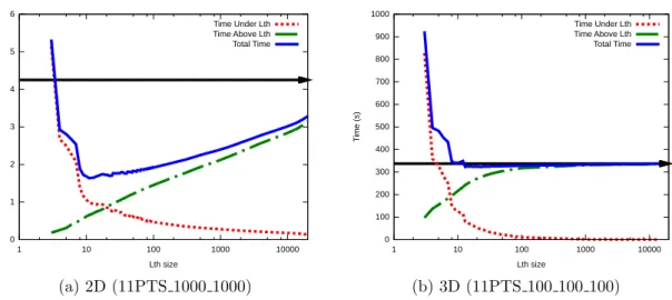
4.2.2 Simulation 0 1 2 3 4 5 6 1 10 100 1000 10000 Ti m e (s) Lth size Time Under Lth Time Above Lth Total Time (a) 2D (11PTS 1000 1000) 0 100 200 300 400 500 600 700 800 900 1000 1 10 100 1000 10000 Ti m e (s) Lth size Time Under Lth Time Above Lth Total Time (b) 3D (11PTS 100 100 100)
Figure 4: 2D vs 3D: Simulated time as a function of the number of nodes in the Lth layer for
two matrices of order 1 million for the AlgTime algorithm.
Before an actual implementation, we made some simulations in order to predict the effective-ness of our approach. The simulator was written in the Python programming language and relies on the performance model described above. Figure 4 shows results obtained for two different ma-trices generated from a finite-difference discretization. The 2D matrix uses a 9-point stencil on a square and the 3D matrix uses an 11-point stencil on a cube. We have chosen these two matrices because they represent typical cases of regular problems, with very different characteristics. The elimination tree related to the 2D matrix contains many small nodes at its bottom while nodes at the top are not very large comparatively. On the other hand, the elimination tree related to the 3D matrix contains nodes with a rapidly increasing size from bottom to top. Simulations consisted in estimating the time spent under and above Lth, as well as the total factorization
time, for all layers possibly reached by the algorithm (until the leaves).
The X-axis corresponds to the number of nodes contained in the different layers and the Y-axis to the estimated factorization time. The horizontal solid line represents the estimated
time that would be spent in using fine-grain node parallelism only (Section 3). The dotted (resp. solid-dotted) curve corresponds to the time spent under (resp. above) the Lth layers.
As expected, the dotted curve decreases and the solid-dotted one increases with the numbers of nodes in the layers. The solid curve giving the total time (sum of the dotted and solid-dotted curves) seems to have a unique global minimum. We have run several simulations on several matrices and this behavior has been observed on all test cases.
The best Lth is obtained when the solid curve reaches its minimum. Hence, the difference
between the horizontal line and the minimum of the solid curve represents the potential gain provided by the proposed AlgTime algorithm. This gain heavily depends on the kind of matrix, with large 3D problems such as the one from Figure 4 showing the smallest potential for Lth
-based algorithms exploiting tree parallelism: the smaller the fronts in the matrix, the better the gain we can expect from tree parallelism. This is the reason why there is a gap between the solid curve and the horizontal line at the right-most of the 2D problem in Figure 4, where Lth contains
all leaves. This gap represents the gain of using tree parallelism on the leaves of the tree.
4.3
Implementation
Algorithm 6 Factorization phase using the Lth-based algorithms.
1: 1. Process nodes underLth (tree parallelism)
2: for all subtrees S, starting from the most costly ones, in parallel do
3: for all nodes N ∈ S, following a postorder do
4: Assemble, factorize and stack the frontal matrix of N , using one thread (Algorithms 1, 2 and 3)
5: end for
6: end for
7: Wait for the other threads
8: Compute global information (reduction operations)
9: 2. Perform computations aboveLth (node parallelism)
10: for all nodes N above Lth do
11: Assemble, factorize and stack the frontal matrix of N , using all threads (Algorithms 1, 2
and 3)
12: end for
The factorization algorithm (Algorithm 6) consists of two phases: first, Lth subtrees are
pro-cessed using tree parallelism; then, the nodes above Lth are processed using node parallelism.
At line 2 of the algorithm, each thread dynamically extracts the next most costly subtree. We have also implemented a static variant that follows the tentative mapping from the analysis phase. One important aspect of our approach is that we were able to directly call the com-putational kernels (assembly, factorization and stacking) and memory management routines of our existing solver. A possible risk is that, because the kernels use OpenMP themselves, calling them inside an OpenMP parallel region could generate many more threads than the number of cores available. This is not occurring when nested parallelism is disabled (this can be forced by using omp set nested(.false.)) and the existing kernels are executed sequentially within a nested region. Enabling OMP DYNAMIC by a call omp set dynamic (.true.) also avoids creating too many threads inside a nested region. Finally, another possibility simply consists in explicitly setting the number of threads to one inside the loop on Lth subtrees.
We now discuss memory management. As said in Section 2.1, in our environment, one very large array is allocated once that will be used as workspace for all frontal matrices, factors and
stack of contribution blocks. Keeping a single work array for all threads (and for the top of the tree) is not a straightforward approach because the existing memory management algorithms do not easily generalize to multiple threads. First, the stack of contribution blocks is no more a stack when working with multiple threads. Second, the threads under Lth would require
synchronizations for the reservation of their private fronts or contribution blocks in the work array; due to the very large number of fronts in the elimination tree, these synchronizations would be very costly. Third, smart memory management schemes including in-place assemblies and compression of factors have been developed in order to minimize the memory consumption, that would not generalize if threads work in parallel on the same work array. In order to avoid these difficulties, use the existing memory management routines without modification, and possibly be more cache-friendly, we have decided to create one private workspace for each thread, under Lth, and still use the same shared workspace above Lth (although smaller than before since
only the top of the tree is concerned). This approach raises a minor issue. Before factorizing a front, contribution blocks of its children must be assembled in it (Algorithm 1). This is not completely straightforward for the parents of the Lth fronts because different threads may handle
different children of this parent front. We thus need to keep track of which thread handles which subtree under Lth, so that one can locate the contribution blocks in the proper thread-private
workspaces. This modification of the assembly algorithm is the only modification that had to be done to the existing kernels implementing Algorithms 1, 2 and 3. Remark that, when all contribution blocks in a local workspace have been consumed, it could be worth decreasing the size of the workspace so that only the memory pages containing the factors remain in memory. Depending on platforms, this can be done with the realloc routine.
Finally, local statistics are computed for each thread in private variables (number of opera-tions, largest front size, etc.) and are reduced before switching from tree to node parallelism in the upper part of the tree, where they will also be updated by the main thread.
4.4
Experiments
We can see in Table 3 that Lth-based algorithms improve the factorization time of all sparse
matrices, in addition to the improvements previously discussed in Section 3. Lth-based algorithms
applied in a pure shared-memory environment also result in a better performance than when message-passing is used (see the results from Table 2).
We first observe that the gains of the proposed algorithms are very important on matrices whose elimination trees present the same characteristics as those of the 2D matrix presented above, namely: trees with many nodes at the bottom and few medium-sized nodes at the top. Such matrices arise, for example, from 2D finite-element and circuit-simulation problems. In those cases, the gain offered by Lth-based algorithms seems independent from the size of the
matrices. For the entire 2D GeoAzur set, the total factorization time has been divided by a factor of two. In the case of matrices whose elimination trees present the characteristics similar to those of the 3D case presented above, the proposed Lth-based algorithms still manage to offer
a gain. However, gains are generally much smaller than those observed in the 2D case. The reason for the difference of effectiveness between 3D-like and 2D-like problems is that, in the 3D case, most of the time is spent above Lthbecause the fronts in this region are very large, whereas
in the 2D case, a significant proportion of the work is spent on small frontal matrices under Lth.
An extreme case is the QIMONDA07 matrix (from circuit simulation), where fronts are very small in all the regions of the elimination tree, with an overhead in multithreaded executions leading to speed-downs. Thus, AlgTime is extremely effective on such a matrix. On this matrix, the AlgFlops algorithm aiming at balancing the work under Lth was not able to find a good
Threaded Lth-based
Serial BLAS + algorithms Matrix reference OpenMP AlgFlops AlgTime 3Dspectralwave 2061.95 371.87 343.64 339.78 AUDI 1270.20 249.21 225.82 210.10 sparsine 314.58 61.87 59.46 57.91 ultrasound80 441.84 89.16 77.06 77.85 dielFilterV3real 271.96 59.31 46.10 44.52 Haltere 691.72 120.81 102.17 99.51 ecl32 3.00 1.05 3.07 0.72 G3 circuit 16.99 8.73 8.82 3.02 QIMONDA07 25.78 28.49 27.34 4.26 GeoAzur 3D 32 32 32 75.74 15.84 13.02 12.87 GeoAzur 3D 48 48 48 410.78 72.96 64.14 62.48 GeoAzur 3D 64 64 64 1563.01 254.38 228.69 228.12 GeoAzur 2D 512 512 4.48 2.33 0.88 0.84 GeoAzur 2D 1024 1024 30.97 11.65 5.37 5.02 GeoAzur 2D 2048 2048 227.08 64.27 35.47 34.56 Table 3: Experimental results with Lth-based algorithms on hidalgo (8 cores).
As predicted by the simulations of Section 4.2.2, the loss of time due to the synchronization of the threads on Lth before starting the factorization above Lth is largely compensated by the
gain of applying mono-threaded factorizations under Lth. This is a key aspect. It shows that,
in multi-core environments, making threads work on separate tasks is better than making them collaborate on the same tasks, even at the price of a strong synchronization. We will discuss a simple strategy to further reduce the overhead due to such a synchronization in Section 6.
In the case of homogeneous subtrees under Lth, the difference in execution time between the
AlgFlopsand the AlgTime algorithms is small. Still, AlgTime is more efficient and the gap grows with the problem size. We now analyze the behaviour of the AlgFlops vs AlgTime algorithms in more details by making the following three observations.
• AlgTime induces a better load balance of the threads under Lththan does AlgFlops. For
the AUDI matrix, the difference between the completion time of the first and last threads under Lth, when using AlgFlops, is 90.22 − 72.50 = 17.72 seconds, whereas the difference
when using AlgTime is 94.77 − 82.06 = 12.71 seconds. This difference is valuable since less time is wasted for a synchronization purpose.
• the Lth layer obtained with the AlgTime algorithm is higher in the elimination tree than
that of the AlgFlops algorithm. For the AUDI matrix, the Lthof AlgFlops contains 24
subtrees, whereas that of AlgTime only contains 17 subtrees. This shows that AlgTime naturally detects that the time spent under Lth is more valuable than that spent above, as
long as synchronization times remain reasonable.
• AlgFlops offers a gain in the majority of cases; but can yield catastrophic results, espe-cially when elimination trees are unbalanced. One potential problem is that the threshold set in AlgFlops could not be reached, in which case, the algorithm will loop indefinitely until Lth reaches all the leaves of the tree. In order to avoid this behavior, one method is to
up and that very unbalanced Lth’s could lead to disastrous performance. The AlgTime
al-gorithm is much more robust in such situations and brings important gains. For the ecl32 matrix, for example, the factorization time of AlgFlops is 3.07 seconds whereas that of the algorithm shown in Section 3 was 1.05 seconds. In comparison, AlgTime decreases the factorization time down to 0.72 seconds.
These results show that AlgTime is more efficient and more robust than AlgFlops, and brings significant gains.
5
Memory affinity issues on NUMA architectures
In multi-core environments, two main architectural trends have arisen: SMP and NUMA. SMP (Symmetric MultiProcessor) architectures contain symmetric cores in the sense that the access to any piece of memory costs the same for any given core. On the other hand, NUMA (Non-Uniform Memory Access) architectures contain cores whose memory access cost is different depending on the targeted piece of memory. Such architectures contain many sockets, each composed of a processor containing multiple cores, and local memory banks. Each core in a given socket accesses its local memory preferably, and accesses foreign memory banks with different (worse) costs, depending on the interconnection distance between the processors. Hence, SMP processors are fully connected whereas NUMA processors are partially connected and memory is organized hierarchically. Due to this characteristic, increasing the number of cores in an SMP fashion is of increasing difficulty. Hence, more and more modern architectures are NUMA due to its ease of scalability.
When comparing the estimated simulated time with the effective time spent under Lth, it
appeared that the estimation was optimistic. There are two possible reasons for that. First, the estimation only comprises the factorization time, whereas the effective time also includes assemblies and stack operations. However, the amount of time spent in assemblies is very small compared to the factorization time and is not enough to explain the discrepancy. Second, we have run the benchmarks on unloaded machines in order to obtain precise results. For instance, when we have run the mono-threaded benchmarks, only one CPU core was working, all the others being idle. However, in Lth-based algorithms, all the cores are active under Lth at the
same time. In such a case, resource sharing and racing could be the reason for the observed discrepancy under Lth.
5.1
Performance of dense factorization kernels and NUMA effects
In order to understand the effects of SMP and NUMA architectures on sparse factorizations, we must first understand them on dense factorizations. We first study the effects of the load of the cores on the performance, and then discuss the effects of the memory affinity and allocation policies.
5.1.1 Machine load
The machine load is an effect we did not take into account until now. It depends on many variable parameters that are out of our control, making it difficult to model precisely. However, in the case of the multifrontal method, if we consider the stage when threads work under the Lth
layer, we could consider that these threads are mainly in a factorization phase since, for each dense matrix, the time of factorization dominates that of assembly and stack operations.
In order to study the effects of the machine load, we made an experiment on concurrent
mono-threaded factorizations, in which different threads factorize different matrices with the
same characteristics. Hence, we could vary the number and mapping of the threads as the size of the matrices for observing their effects on the machine load.
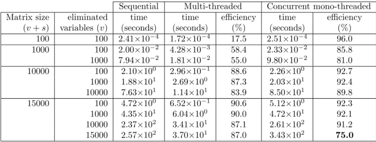
Sequential Multi-threaded Concurrent mono-threaded Matrix size eliminated time time efficiency time efficiency
(v + s) variables (v) (seconds) (seconds) (%) (seconds) (%) 100 100 2.41×10⁻⁴ 1.72×10⁻⁴ 17.5 2.51×10⁻⁴ 96.0 1000 100 2.00×10⁻² 4.28×10⁻³ 58.4 2.33×10⁻² 85.8 1000 7.94×10⁻² 1.81×10⁻² 55.0 9.80×10⁻² 81.0 10000 100 2.10×100 2.96×10⁻¹ 88.6 2.26×100 92.7 1000 1.88×101 2.69×100 87.3 2.03×101 92.4 10000 7.63×101 1.14×101 83.9 8.50×101 89.8 15000 100 4.72×100 6.52×10⁻¹ 90.6 5.12×100 92.3 1000 4.35×101 6.04×100 90.0 4.72×101 92.1 10000 2.37×10² 3.41×101 87.1 2.61×10² 91.2 15000 2.57×10² 3.70×101 87.0 3.43×10² 75.0 Table 4: Factorization times on hidalgo, with varying matrix sizes and varying number of eliminated variables. ’Sequential’ is the execution time for one task using one thread; ’Multi-threaded’ represents the time spent in one task using eight cores, and ’Concurrent mono-’Multi-threaded’ represents the time spent in eight tasks using eight cores.
From the results exposed in Table 4, we can see that, on the hidalgo computer with 8 cores, concurrent mono-threaded factorizations are more efficient than multi-threaded ones. Moreover, concurrent mono-threaded factorizations are always efficient while muti-threaded ones need ma-trices of larger sizes in order to be efficient. We also note that the degradation of performance for both types of factorizations decreases as the number of eliminated variables increases (passing from partial to total factorizations: increasing v for a constant v + s). Surprisingly, we note that in the very special case of the total factorization of the 15000 × 15000 matrix, the performance of concurrent mono-threaded factorizations drops down. This contradicts the usual sense, and shows the limits of the concurrent mono-threaded approach. We can conclude by saying that the degradation in performance is between 5% and 20% in the majority of cases we could encounter under an Lth when applying an Lth-based algorithm, but can reach up to 33% in very unusual
cases.
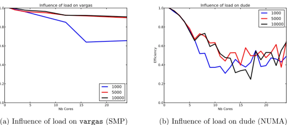
From the results exposed in Figure 5, we can see how the architectures impact the per-formance. On vargas, which is a NUMA machine with such characteristics that it could be considered as an SMP machine, with nearly uniform memory access, the degradation of perfor-mance is progressive with the number of cores. Also, even if the degradation is important for small matrices (1000×1000), it becomes negligible for large ones (5000×5000 and 10000×10000). On dude though, we observe a very rapid degradation of performance independently of the size of the matrices. When choosing the cores on the same processor (6 first cores), the degradation is very smooth and predictable. However, once cores of different processors are used, the trend of the degradation becomes extremely chaotic.
0 5 10 15 20 Nb Cores 0.0 0.2 0.4 0.6 0.8 1.0 Efficiency
Influence of load on vargas
1000 5000 10000
(a) Influence of load on vargas (SMP)
0 5 10 15 20 Nb Cores 0.0 0.2 0.4 0.6 0.8 1.0 Efficiency
Influence of load on dude
1000 5000 10000
(b) Influence of load on dude (NUMA) Figure 5: Influence of machine load on a SMP machine (vargas, 32 cores) and on a NUMA machine (dude, 24 cores). The X-axis represents the number of cores involved in the ’concurrent mono-threaded’ factorization, and the Y-axis represents the efficiency compared to an unloaded machine.
5.1.2 Memory locality and memory interleaving
The more a machine has NUMA effects, the more the cost of memory accesses to a given memory zone will be unbalanced among the processors. Thus, the way a dense matrix is mapped over the memory banks has important consequences on the performance on the factorization time. In Table 5, we extracted the main results of an experiment consisting in factorizing with Algorithm 2 a matrix of size 4000 × 4000 with v = 1000 variables to eliminate and a Schur complement of size s = 3000 with all possible combinations of cores used and memory allocation policies. From these Core ID membind 0 membind 1 localalloc (OS default) interleave 0,1 node 0 0 4.77 4.82 4.78 4.79 1 4.74 4.78 4.73 4.75 0. . . 3 1.39 1.44 1.39 1.37 node 1 4 4.75 4.71 4.71 4.72 4. . . 7 1.44 1.39 1.39 1.37 node 0,1 all 1.10 1.11 1.09 0.79
Table 5: Effect of the locallaloc and interleave policies with different core configurations on hidalgo. The factorization times (seconds) are reported for a matrix of size 4000 with v = 1000 variables to eliminate. membind 0 (resp. 1) forces data allocation on the memory bank of node 0 (resp.1). hidalgo are in seconds on hidalgo of the factorization of a matrix of size 4000 and with v = 1000 eliminated variables with different core configurations.
results, we note that the localalloc policy (allocating memory on the same node as the core asking for it) is the best policy when dealing with serial factorizations. However, the interleave policy (interleaving pages on the memory banks in a round-robin manner) becomes the best one when dealing with multi-threaded factorizations, even when threads are mapped on cores of the same processor. However, this is partially due to the fact that the experiment was done on an
unloaded machine: taking advantage from unused resources from the idle neighbour processors is preferable to overwhelming local socket resources (memory banks, memory bus, caches, . . . ). When running the experiment on all cores, the interleave policy is by far the best one, and brings a huge gain over the local policies. Further experiments made with various matrix sizes and on the dude machine confirm this result.
Therefore, it seems that the best solution when working under Lth with concurrent
mono-threaded factorizations is to allocate thread-private workspaces locally. On the other hand, when working above Lth with multi-threaded factorizations, it will be preferable to allocate the shared
workspace using the interleave policy.
5.2
Application to sparse matrix factorizations
Controlling the memory policy can be done in several ways. A first, non intrusive one, consists in using the numactl utility. However, this utility sets the policy for all the allocations in the program. The second, more intrusive, approach consists in using the libnuma or hwloc [9] libraries. Inside the program, it is then possible to dynamically change the allocation policy. In order to apply the interleave policy only for the workspace shared by all processors above Lth,
while keeping the default localalloc policy for other allocations, in particular for the data local to each thread under Lth, the second approach is necessary. However, applying the desired policy
for each allocation is not enough to improve performance. A profiling of the memory mapping of the shared workspace’s pages shows that the interleave policy is not applied at all. The reason is that when calling the malloc function to allocate a large array, only its first page is actually allocated, and the remaining pages are only allocated when an element of the array corresponding to that page is accessed for the first time. In order to effectively apply the interleave policy, one solution consists in accessing (writing one element of) each page of the array immediately after the allocation. Another portable solution that does not depend on external libraries is to make all threads access all pages that should be allocated on the same socket. Making this small modification dramatically improves the performance of the factorization, as will be discussed in Section 5.3.
Remark that the previous approach forces one to allocate all the pages of the shared workspace at once, while the physical memory also needs to hold the already allocated private workspaces. In the standard approach, memory pages related to the shared workspace are allocated only when needed. At the same time, we would like pages of private workspaces to be gradually recycled to pages of the shared workspace, allowing for a better usage of memory (see remark on realloc in Section 4.3). In general, the first-touch principle applies, which states that, with the localalloc memory allocation policy, a page is allocated on the same node as the thread that first touches it. While working on the parallelization of assembly operations (Algorithm 1), we observed that even without the interleave policy, it was possible to better share the memory pages between the threads by parallelizing the initialization of the frontal matrix to zero. While this had no effect on the time spent in assemblies, significant gains were observed regarding the performance of the factorization (Algorithm 2). Although those gains were not as large as the ones observed with the interleave policy (which are the ones we present in Section 5.3), this approach is an interesting alternative.
5.3
Performance analysis
5.3.1 Effects of the interleave policy
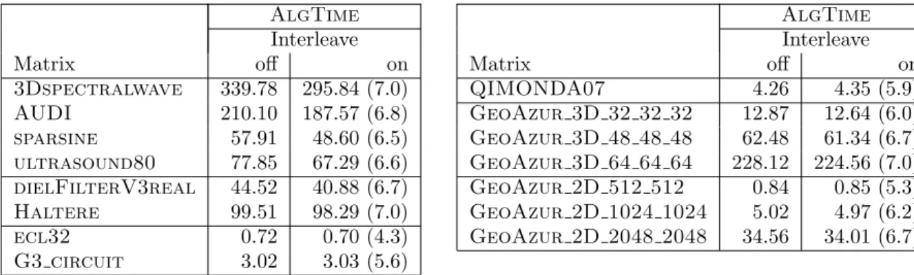
Table 6 shows the factorization time obtained on the hidalgo machine when using the interleave policy above Lth with the AlgTime algorithm. Column “Interleave/off” is identical to the last
column of Table 3. The gains are significant for all matrices except for the smallest problems and for the ones with too small frontal matrices, where interleaving does not help (as could be ex-pected). In Table 7, we analyze further the impact of the interleave memory allocation policy AlgTime AlgTime Interleave Interleave Matrix off on Matrix off on 3Dspectralwave 339.78 295.84 (7.0) QIMONDA07 4.26 4.35 (5.9) AUDI 210.10 187.57 (6.8) GeoAzur 3D 32 32 32 12.87 12.64 (6.0) sparsine 57.91 48.60 (6.5) GeoAzur 3D 48 48 48 62.48 61.34 (6.7) ultrasound80 77.85 67.29 (6.6) GeoAzur 3D 64 64 64 228.12 224.56 (7.0) dielFilterV3real 44.52 40.88 (6.7) GeoAzur 2D 512 512 0.84 0.85 (5.3) Haltere 99.51 98.29 (7.0) GeoAzur 2D 1024 1024 5.02 4.97 (6.2) ecl32 0.72 0.70 (4.3) GeoAzur 2D 2048 2048 34.56 34.01 (6.7) G3 circuit 3.02 3.03 (5.6)
Table 6: Factorization times (seconds) without with the interleave policy on the factorization time with the AlgTime algorithm on hidalgo, 8 cores. The numbers in parenthesis correspond to the speed-ups with respect to sequential executions.
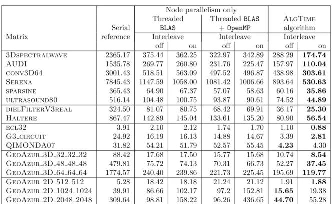
on the dude platform, which has more cores and shows more NUMA effects than hidalgo. The first columns correspond to runs in which only node parallelism is applied, whereas in the last columns, the AlgTime algorithm is applied. Parallel BLAS (“Threaded BLAS”) in Algorithm 2 may be coupled with an OpenMP parallelization of Algorithms 1 and 3 (column “Threaded BLAS + OpenMP”). The first observation is that the addition of OpenMP directives on top of threaded BLAS brings significant gains compared to the use of threaded BLAS alone. We also observe in those cases that the interleave policy alone does not bring so much gain and does even bring losses in a few cases. Then, we used the AlgTime algorithm combined with the interleave policy (above Lth). By comparing the timings in the last two columns, we then observe very
impressive gains with the interleave policy.
These results can be explained by the fact that the interleave policy is harmful on small dense matrices, possibly because when CPU cores of different NUMA nodes collaborate, the cost of cache coherency will be much more important than the price of memory access. On the contrary, on medium-to-large dense matrices, the effects of the interleave policy are beneficial. The Lth layer separating the small fronts (bottom) from the large fronts (top) makes us benefit
from interleaving without its negative effects. This is why the interleave policy alone does not bring much gain, whereas it brings huge gains when combined to the AlgTime algorithm.
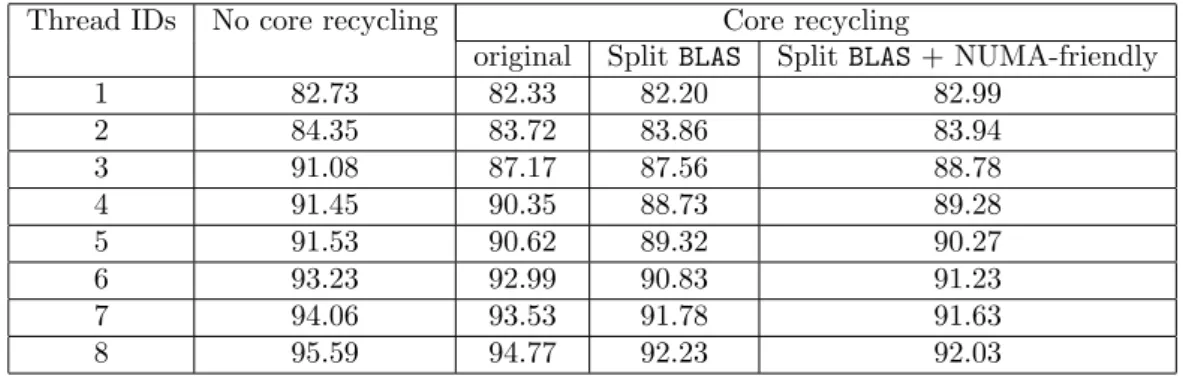
Table 8 shows the time spent under and above Lth, with and without interleaving, with and
without Lth for the AUDI test case. In the first two columns corresponding to node parallelism,
although the Lth layer is not used by the algorithm, we measure the times corresponding to
the Lth layer defined by the AlgTime algorithm from the last two columns. We can see that
Lth-based algorithms improve the time spent under Lth (from 109.81 seconds to 36.02 seconds)
thanks to tree parallelism; above, the time is identical since only node parallelism is used in both cases. When using the interleave policy, we can see that the time above Lth decreases
a lot (from 121.95 seconds to 73.93 seconds) but that this is not the case for the time under Lth. Moreover, we note that using the interleave policy without using Lth-based algorithms is
disastrous for the performance under the Lth layer (from 109.81 seconds to 151.54 seconds). This
confirms that the interleave policy should not be used on small frontal matrices, especially in parallel.