Structures algébriques, systèmes superintégrables et polynômes orthogonaux

(1)

Université de Montréal

Structures algébriques, systèmes superintégrables et

polynômes orthogonaux

par

Vincent Genest

Département de physique Faculté des arts et des sciences

Thèse présentée à la Faculté des études supérieures en vue de l’obtention du grade de

Philosophiæ Doctor (PhD) en physique

19 mai 2015

(2)

Université de Montréal

Faculté des études supérieures

Cette thèse intitulée

Structures algébriques, systèmes superintégrables

et polynômes orthogonaux

présentée par

Vincent Genest

a été évaluée par un jury composé des personnes suivantes:

Richard MacKenzie

Président-rapporteur

Luc Vinet

Directeur de recherche

Yvan Saint-Aubin

Membre du jury

Nicolai Reshetikhin

Examinateur externe Thèse acceptée le : 8 juin 2015

(3)

Résumé

Cette thèse est divisée en cinq parties portant sur les thèmes suivants: l’interprétation physique et algébrique de familles de fonctions orthogonales multivariées et leurs applica-tions, les systèmes quantiques superintégrables en deux et trois dimensions faisant inter-venir des opérateurs de réflexion, la caractérisation de familles de polynômes orthogonaux appartenant au tableau de Bannai–Ito et l’examen des structures algébriques qui leurs sont associées, l’étude de la relation entre le recouplage de représentations irréductibles d’algèbres et de superalgèbres et les systèmes superintégrables, ainsi que l’interprétation algébrique de familles de polynômes multi-orthogonaux matriciels.

Dans la première partie, on développe l’interprétation physico-algébrique des familles de polynômes orthogonaux multivariés de Krawtchouk, de Meixner et de Charlier en tant qu’éléments de matrice des représentations unitaires des groupes SO(d + 1), SO(d,1) et E(d) sur les états d’oscillateurs. On détermine les amplitudes de transition entre les états de l’oscillateur singulier associés aux bases cartésienne et polysphérique en termes des polynômes multivariés de Hahn. On examine les coefficients 9 j de su(1, 1) par le biais du système superintégrable générique sur la 3-sphère. On caractérise les polynômes de q-Krawtchouk comme éléments de matrices des « q-rotations » de Uq(sl2). On conçoit

un réseau de spin bidimensionnel qui permet le transfert parfait d’états quantiques à l’aide des polynômes de Krawtchouk à deux variables et on construit un modèle discret de l’oscillateur quantique dans le plan à l’aide des polynômes de Meixner bivariés.

Dans la seconde partie, on étudie les systèmes superintégrables de type Dunkl, qui font intervenir des opérateurs de réflexion. On examine l’oscillateur de Dunkl en deux et trois dimensions, l’oscillateur singulier de Dunkl dans le plan et le système générique sur la 2-sphère avec réflexions. On démontre la superintégrabilité de chacun de ces systèmes. On obtient leurs constantes du mouvement, on détermine leurs algèbres de symétrie et leurs représentations, on donne leurs solutions exactes et on détaille leurs liens avec les polynômes orthogonaux du tableau de Bannai–Ito.

(4)

Dans la troisième partie, on caractérise deux familles de polynômes du tableau de Bannai–Ito: les polynômes de Bannai–Ito complémentaires et les polynômes de Chihara. On montre également que les polynômes de Bannai–Ito sont les coefficients de Racah de la superalgèbre osp(1|2). On détermine l’algèbre de symétrie des polynômes duaux −1 de Hahn dans le cadre du problème de Clebsch-Gordan de osp(1|2). On propose une q-généralisation des polynômes de Bannai–Ito en examinant le problème de Racah pour la superalgèbre quantiqueosp_q_{(1|2). Finalement, on montre que la q-algèbre de Bannai–Ito}

sert d’algèbre de covariance àosp_q(1|2).

Dans la quatrième partie, on détermine le lien entre le recouplage de représenta-tions des algèbressu(1, 1) etosp(1|2) et les systèmes superintégrables du deuxième ordre avec ou sans réflexions. On étudie également les représentations des algèbres de Racah– Wilson et de Bannai–Ito. On montre aussi que l’algèbre de Racah–Wilson sert d’algèbre de covariance quadratique à l’algèbre de Liesl(2).

Dans la cinquième partie, on construit deux familles explicites de polynômes d-ortho-gonaux basées sursu(2). On étudie les états cohérents et comprimés de l’oscillateur fini et on caractérise une famille de polynômes multi-orthogonaux matriciels.

Mot-clefs

• Polynômes orthogonaux • Systèmes superintégrables • Algèbres quadratiques • Tableau de Bannai–Ito • Opérateurs de Dunkl

(5)

Abstract

This thesis is divided into five parts concerned with the following topics: the physical and algebraic interpretation of families of multivariate orthogonal functions and their applications, the study of superintegrable quantum systems in two and three dimensions involving reflection operators, the characterization of families of orthogonal polynomials of the Bannai-Ito scheme and the study of the algebraic structures associated to them, the investigation of the relationship between the recoupling of irreducible representations of algebras and superalgebras and superintegrable systems, as well as the algebraic inter-pretation of families of matrix multi-orthogonal polynomials.

In the first part, we develop the physical and algebraic interpretation of the Kraw-tchouk, Meixner and Charlier families of multivariate orthogonal polynomials as matrix elements of unitary representations of the SO(d + 1), SO(d,1) and E(d) groups on oscil-lator states. We determine the transition amplitudes between the states of the singular oscillator associated to the Cartesian and polyspherical bases in terms of the multivariate Hahn polynomials. We examine the 9 j coefficients ofsu(1, 1) through the generic super-integrable system on the 3-sphere. We characterize the q-Krawtchouk polynomials as matrix elements of “q-rotations” of Uq(sl2). We show how to design a two-dimensional

spin network that allows perfect state transfer using the two-variable Krawtchouk poly-nomials and we construct a discrete model of the two-dimensional quantum oscillator using the two-variable Meixner polynomials.

In the second part, we study superintegrable systems of Dunkl type, which involve reflections. We examine the Dunkl oscillator in two and three dimensions, the singular Dunkl oscillator in the plane and the generic system on the 2-sphere with reflections. We show that each of these systems is superintegrable. We obtain their constants of motion, we find their symmetry algebras as well as their representations, we give their exact solutions and we exhibit their relationship with the orthogonal polynomials of the Bannai–Ito scheme.

(6)

In the third part, we characterize two families of polynomials belonging to the Bannai– Ito scheme: the complementary Bannai-Ito polynomials and the Chihara polynomials. We also show that the Bannai–Ito polynomials arise as Racah coefficients for theosp(1|2) superalgebra. We determine the symmetry algebra associated with the dual −1 Hahn polynomials in the context of the Clebsch-Gordan problem for osp(1|2). We introduce a q-generalization of the Bannai-Ito polynomials by examining the Racah problem for the quantum superalgebra osp_q_{(1|2). Finally, we show that the q-deformed Bannai-Ito}

algebra serves as a covariance algebra forosp_q(1|2).

In the fourth part, we determine the relationship between the recoupling of repre-sentations of thesu(1, 1) andosp(1|2) algebras and second-order superintegrable systems with or without reflections. We also study representations of Racah–Wilson and Bannai– Ito algebras. Moreover, we show that the Racah–Wilson algebra serves as a quadratic covariance algebra forsl(2).

In the fifth part, we explicitly construct two families of d-orthogonal polynomials based on su(2). We investigate the squeezed/coherent states of the finite oscillator and we characterize a family of matrix multi-orthogonal polynomials.

Keywords

• Orthogonal polynomials • Superintegrable systems • Quadratic algebras • Bannai–Ito scheme • Dunkl operators

(7)

Table des matières

Introduction 1

I

Polynômes orthogonaux multivariés et applications

7

Introduction 9

1 The multivariate Krawtchouk polynomials as matrix elements of the

rotation group representations on oscillator states 13

1.1 Introduction . . . 14

1.2 Representations of SO(3) on the quantum states of the harmonic os-cillator in three dimensions . . . 17

1.2.1 The Weyl algebra . . . 17

1.2.2 The 3D quantum harmonic oscillator . . . 18

1.2.3 The representations of SO(3) ⊂ SU(3) on oscillator states . . . . 19

1.3 The representation matrix elements as orthogonal polynomials . . . 20

1.3.1 Calculation of the amplitude Wi,k;N . . . 21

1.3.2 Raising relations . . . 22

1.3.3 Orthogonality relation . . . 22

1.3.4 Lowering relations . . . 23

1.4 Duality . . . 23

1.5 Generating function . . . 24

1.6 Recurrence relations and difference equations . . . 27

1.6.1 Recurrence relations . . . 27

1.6.2 Difference equations . . . 28

(8)

1.8 Rotations in coordinate planes

and univariate Krawtchouk polynomials . . . 30

1.9 The bivariate Krawtchouk-Tratnik as special cases . . . 33

1.10 Addition formulas . . . 34

1.10.1 General addition formula . . . 35

1.10.2 The Tratnik expression . . . 35

1.10.3 Expansion of the general Krawtchouk polynomials in the Krawtchouk-Tratnik polynomials . . . 36

1.11 Multidimensional case . . . 37

1.12 Conclusion . . . 39

1.A Background on multivariate Krawtchouk polynomials . . . 40

References . . . 45

2 The multivariate Meixner polynomials as matrix elements of SO(d, 1) representations on oscillator states 49 2.1 Introduction . . . 49

2.2 Representations of SO(2, 1) on oscillator states . . . 51

2.3 The representation matrix elements as orthogonal polynomials . . . . 53

2.3.1 Calculation of W_i,k(β). . . 54

2.3.3 Orthogonality Relation . . . 55

2.3.4 Lowering Relations . . . 56

2.4 Duality . . . 56

2.5 Generating function and hypergeometric expression . . . 57

2.5.1 Generating function . . . 57

2.5.2 Hypergeometric expression . . . 59

2.7 One-parameter subgroups and univariate Meixner & Krawtchouk polynomials . . . 61

(9)

2.7.1 Hyperbolic subgroups: Meixner polynomials . . . 62

2.7.2 Elliptic subgroup: Krawtchouk polynomials . . . 64

2.8 Addition formulas . . . 65

2.8.1 General addition formula . . . 65

2.8.2 Special case I: product of two hyperbolic elements . . . 65

2.8.3 General case . . . 66

2.9 Multivariate case . . . 67

References . . . 70

3 The multivariate Charlier polynomials as matrix elements of the Euclidean group representation on oscillator states 73 3.1 Introduction . . . 74

3.2 Representation of E(2) on oscillator states . . . 75

3.2.1 The Heisenberg-Weyl algebra . . . 75

3.2.2 The two-dimensional isotropic oscillator . . . 76

3.2.3 Representation of E(2) on oscillator states . . . 77

3.3 The representation matrix elements as orthogonal polynomials . . . . 78

3.3.1 Calculation of W . . . 79 3.3.2 Raising relations . . . 79 3.3.3 Orthogonality relation . . . 80 3.3.4 Lowering relations . . . 80 3.4 Duality . . . 81 3.5 Generating function . . . 82

3.6 Explicit expression in hypergeometric series . . . 83

3.8 Explicit expression in standard Charlier and Krawtchouk polynomials . . . 85

3.9 Integral representation . . . 86

3.10 Charlier polynomials as limits of Krawtchouk polynomials . . . 87

(10)

3.10.2 Limit of bivariate Krawtchouk polynomials . . . 88

3.11 Multidimensional case . . . 89

References . . . 92

4 Interbasis expansions for the isotropic 3D harmonic oscillator and bivariate Krawtchouk polynomials 95 4.1 Introduction . . . 95

4.1.1 Three-dimensional isotropic harmonic oscillator . . . 96

4.1.2 SO(3) ⊂ SU(3) and oscillator states . . . 97

4.1.3 Unitary representations of SO(3) and bivariate Krawtchouk polynomials . . . 98

4.1.4 The main result . . . 100

4.1.5 Outline . . . 102

4.2 Thesu(1, 1) Lie algebra and the Clebsch-Gordan problem . . . 102

4.2.1 Thesu(1, 1) algebra and its positive-discrete series of representations . . . 102

4.2.2 The Clebsch-Gordan problem . . . 103

4.2.3 Explicit expression for the Clebsch-Gordan coefficients . . . 104

4.3 Overlap coefficients for the isotropic 3D harmonic oscillator . . . 106

4.3.1 The Cartesian/polar overlaps . . . 106

4.3.2 The polar/spherical overlaps . . . 108

References . . . 112

5 The multivariate Hahn polynomials and the singular oscillator 115 5.1 Introduction . . . 115

5.2 The three-dimensional singular oscillator . . . 118

5.2.1 Hamiltonian and spectrum . . . 118

5.2.2 The Cartesian basis . . . 118

5.2.3 The spherical basis . . . 119

5.2.4 The main object . . . 121 5.3 The expansion coefficients as orthogonal polynomials in two variables 122

(11)

5.3.1 Calculation of W(α1,α2,α3) i,k;N . . . 122 5.3.2 Raising relations . . . 123 5.3.3 Orthogonality relation . . . 125 5.3.4 Lowering relations . . . 126 5.4 Generating function . . . 128 5.5 Recurrence relations . . . 130

5.5.1 Forward structure relation in the variable i . . . 130

5.5.2 Backward structure relation in the variable i . . . 131

5.5.3 Forward and backward structure relations in the variable k . . . 132

5.5.4 Recurrence relations for the polynomials Q(α1,α2,α2) m,n (i, k; N) . . . 133

5.6 Difference equations . . . 134

5.6.1 First difference equation . . . 135

5.6.2 Second difference equation . . . 136

5.7 Expression in hypergeometric series . . . 137

5.7.1 The cylindrical-polar basis . . . 137

5.7.2 The cylindrical/Cartesian expansion . . . 138

5.7.3 The spherical/cylindrical expansion . . . 139

5.7.4 Explicit expression for Q(α1,α2,α3) m,n (i, k; N) . . . 140

5.8 Algebraic interpretation . . . 140

5.8.1 Generalized Clebsch-Gordan problem forsu(1, 1) . . . 141

5.8.2 Connection with the singular oscillator . . . 142

5.9 Multivariate case . . . 144

5.9.1 Cartesian and hyperspherical bases . . . 144

5.9.2 Interbasis expansion coefficients as orthogonal polynomials . . . 146

5.A A compendium of formulas for the bivariate Hahn polynomials . . . 148

5.A.1 Definition . . . 148

5.A.2 Orthogonality . . . 148

5.A.3 Recurrence relations . . . 149

5.A.4 Difference equations . . . 150

5.A.5 Generating Function . . . 150

5.A.6 Forward shift operators . . . 150

(12)

5.A.8 Structure relations . . . 151

5.B Structure relations for Jacobi polynomials . . . 152

5.C Structure relations for Laguerre polynomials . . . 153

6 The generic superintegrable system on the 3-sphere and the 9 j symbols ofsu(1, 1) 157 6.1 Introduction . . . 157

6.2 The 9 j problem forsu(1, 1) in the position representation . . . 159

6.2.1 The addition of four representations and the generic system on S3 . . . 160

6.2.2 The 9 jsymbols . . . 162

6.2.3 The canonical bases by separation of variables . . . 163

6.2.4 9 j symbols as overlap coefficients, integral representation and symmetries . . . 166

6.3 Double integral formula and the vacuum 9 j coefficients . . . 167

6.3.1 Extension of the wavefunctions . . . 168

6.3.2 The vacuum 9 j coefficients . . . 169

6.4 Raising, lowering operators and contiguity relations . . . 171

6.4.1 Raising, lowering operators and factorization . . . 171

6.4.2 Contiguity relations . . . 172

6.4.3 9 j symbols and rational functions . . . 176

6.5 Difference equations and recurrence relations . . . 178

6.A Properties of Jacobi polynomials . . . 183

6.B Action of A(α1,α2) − onΞ (α1,α2,α3,α4) x, y;N . . . 184 6.C Action of A(α1−1,α2−1) + onΞ (α1,α2,α3,α4) x, y;N . . . 186 References . . . 188

7 q-Rotations and Krawtchouk polynomials 193 7.1 Introduction . . . 193

(13)

7.2.1 Elements of q-analysis . . . 195

7.2.2 The Schwinger model forUq(sl2) . . . 196

7.2.3 Unitary q-rotation operators and matrix elements . . . 197

7.3 Matrix elements and self-duality . . . 199

7.3.1 Matrix elements and quantum q-Krawtchouk polynomials . . . 199

7.3.2 Duality . . . 201

7.3.3 The q ↑ 1 limit . . . 202

7.4 Structure relations . . . 202

7.4.1 Backward relation . . . 202

7.4.2 Forward relation . . . 203

7.4.3 Dual backward and forward relations . . . 204

7.5 Generating function . . . 204

7.5.1 Generating function with respect to the degrees . . . 204

7.5.2 Generating function with respect to the variables . . . 206

7.6 Recurrence relation and difference equation . . . 207

7.6.1 Recurrence relation . . . 207

7.6.2 Difference equation . . . 208

7.7 Duality relation with affine q-Krawtchouk polynomials . . . 209

8 Spin lattices, state transfer and bivariate Krawtchouk polynomials 215 8.1 Introduction . . . 215

8.2 Triangular spin lattices and one-excitation dynamics . . . 217

8.3 Representations of O(3) on oscillator states and orthogonal polynomials 218 8.3.1 Calculation of Ws,t;N . . . 219

8.3.3 Orthogonality relation . . . 221

8.4 Recurrence relations and exact solutions of 1-excitation dynamics . . . 221

8.5 State transfer . . . 223

(14)

9 A superintegrable discrete oscillator and two-variable Meixner poly-nomials 229 9.1 Introduction . . . 229

9.2 The two-variable Meixner polynomials . . . 232

9.3 A discrete and superintegrable Hamiltonian . . . 234

9.4 Continuum limit to the standard oscillator . . . 236

9.4.1 Continuum limit of the two-variable Meixner polynomials . . . . 237

9.4.2 Continuum limit of the raising/lowering operators . . . 240

II

Systèmes superintégrables avec réflexions

245

Introduction 247 10 The Dunkl oscillator in the plane I : superintegrability, separated wavefunctions and overlap coefficients 249 10.1 Introduction . . . 250

10.2 The model and exact solutions . . . 251

10.2.1 Solutions in Cartesian coordinates . . . 252

10.2.2 Solutions in polar coordinates . . . 253

10.2.3 Separation of variables and Jacobi-Dunkl polynomials . . . 256

10.3 Superintegrability . . . 259

10.3.1 Dynamical algebra and spectrum . . . 259

10.3.2 Superintegrability and the Schwinger-Dunkl algebra . . . 260

10.4 Overlap Coefficients . . . 262

10.4.1 Overlap coefficients for sxsy= +1 . . . 262

10.4.2 Overlap coefficients for sxsy= −1 . . . 266

10.5 The Schwinger-Dunkl algebra and the Clebsch-Gordan problem . . . 269

10.5.1 sl₋₁(2) Clebsch–Gordan coefficients and overlap coefficients . . . 269

10.5.2 Occurrence of the Schwinger-Dunkl algebra . . . 271

(15)

10.A Appendix A . . . 272

10.A.1 Formulas for Laguerre polynomials . . . 272

10.A.2 Formulas for Jacobi polynomials . . . 272

10.A.3 Formulas for dual −1 Hahn polynomials . . . 272

10.B Appendix B . . . 273

11 The Dunkl oscillator in the plane II : representations of the symmetry algebra 279 11.1 Introduction . . . 280

11.1.1 Superintegrability . . . 280

11.1.2 The Dunkl oscillator model . . . 280

11.1.3 Symmetries of the Dunkl oscillator . . . 281

11.1.4 The main object: the Schwinger-Dunkl algebra sd(2) . . . 282

11.1.5 Outline . . . 283

11.2 The Cartesian basis . . . 283

11.3 The circular basis . . . 286

11.3.1 Transition matrix from the circular to the Cartesian basis . . . 288

11.3.2 Matrix representation of J2and spectrum . . . 289

11.4 Diagonalization of J2: the N even case . . . 292

11.4.1 The operatorQ and its simultaneous eigenvalue equation . . . . 292

11.4.3 Generating function and Heun polynomials . . . 296

11.4.4 Expansion of Heun polynomials in the complementary Bannai-Ito polynomials . . . 298

11.4.5 Eigenvectors of J2 . . . 300

11.4.6 The fully isotropic case . . . 301

11.5 Diagonalization of J2: the N odd case . . . 302

11.5.1 The operatorQ and its simultaneous eigenvalue equation . . . . 302

11.5.3 Generating functions and Heun polynomials . . . 306

11.5.4 Expansion of Heun polynomials in complementary Bannai-Ito polynomials . . . 306

(16)

11.5.6 The fully isotropic case : −1 Jacobi polynomials . . . 309

11.6 Representations of sd(2) in the J2eigenbasis . . . 310

11.6.1 The N odd case . . . 310

11.6.2 The N even case . . . 312

12 The singular and the 2 : 1 anisotropic Dunkl oscillators in the plane 317 12.1 Introduction . . . 318

12.2 The singular Dunkl oscillator . . . 320

12.2.1 Hamiltonian, dynamical symmetries and spectrum . . . 320

12.2.2 Exact solutions and separation of variables . . . 323

12.2.3 Integrals of motion and symmetry algebra . . . 327

12.2.4 Symmetries, separability and the Hahn algebra with involutions 328 12.3 The 2 : 1 anisotropic Dunkl oscillator . . . 330

12.3.1 Hamiltonian, dynamical symmetries and spectrum . . . 331

12.3.2 Exact solutions and separation of variables . . . 332

12.3.3 Integrals of motion and symmetry algebra . . . 333

12.3.4 Special case I . . . 334

12.3.5 Special case II . . . 336

13 The Dunkl oscillator in three dimensions 343 13.1 Introduction . . . 343

13.1.2 Dunkl oscillator models in the plane . . . 344

13.1.3 The three-dimensional Dunkl oscillator . . . 345

13.1.4 Outline . . . 346

13.2 Superintegrability . . . 346

13.2.1 Dynamical algebra and spectrum . . . 346

13.2.2 Constants of motion and the Schwinger-Dunkl algebra sd(3) . . . 347

13.2.3 An alternative presentation of sd(3) . . . 349 13.3 Separated Solutions: Cartesian, cylindrical and spherical coordinates 350

(17)

13.3.1 Cartesian coordinates . . . 350

13.3.2 Cylindrical coordinates . . . 352

13.3.3 Spherical coordinates . . . 354

14 The Bannai–Ito algebra and a superintegrable system with reflec-tions on the 2-sphere 359 14.1 Introduction . . . 359

14.2 The model on S2, superintegrability and symmetry algebra . . . 362

14.2.1 The model on S2 . . . 362

14.2.3 Symmetry algebra . . . 363

14.3 Exact solution . . . 365

14.3.1 Standard spherical coordinates . . . 365

14.3.2 Alternative spherical coordinates . . . 367

14.4 Connection with sl₋₁(2) . . . 368

14.4.1 sl₋₁(2) algebra . . . 368

14.4.2 Differential/Difference realization and the model on the 2-sphere . . . 369

14.5 Superintegrable model in the plane from contraction . . . 371

14.5.1 Contraction of the Hamiltonian . . . 371

14.5.2 Contraction of the constants of motion . . . 372

15 A Dirac–Dunkl equation on S2 and the Bannai–Ito algebra 377 15.1 Introduction . . . 377

15.2 Laplace– and Dirac– Dunkl operators forZ3₂ . . . 379

15.2.1 Laplace– and Dirac– Dunkl operators inR3 . . . 379

(18)

15.3 Symmetries of the spherical

Dirac–Dunkl operator . . . 383

15.4 Representations of the Bannai–Ito algebra . . . 384

15.5 Eigenfunctions of the spherical Dirac–Dunkl operator . . . 389

15.5.1 Cauchy-Kovalevskaia map . . . 389

15.5.2 A basis forMN(R3) . . . 390

15.5.3 Basis spinors and representations of the Bannai–Ito algebra . . 393

15.5.4 Normalized wavefunctions . . . 394

15.5.5 Role of the Bannai–Ito polynomials . . . 395

III

Tableau de Bannai–Ito et

structures algébriques associées

399

Introduction . . . 401

16 Bispectrality of the Complementary Bannai–Ito polynomials 403 16.1 Introduction . . . 403

16.2 Bannai–Ito polynomials . . . 405

16.3 CBI polynomials . . . 407

16.4 Bispectrality of CBI polynomials . . . 412

16.5 The CBI algebra . . . 418

16.6 Three OPs families related to the CBI polynomials . . . 422

16.6.1 Dual −1 Hahn polynomials . . . 422

16.6.2 The symmetric Hahn polynomials . . . 424

16.6.3 Para-Krawtchouk polynomials . . . 426

17 A “continuous” limit of the Complementary Bannai–Ito polynomials: Chihara polynomials 431 17.1 Introduction . . . 432

(19)

17.2 Complementary Bannai–Ito polynomials . . . 434

17.3 A “continuous” limit to Chihara polynomials . . . 437

17.4 Bispectrality of the Chihara polynomials . . . 438

17.4.1 Bispectrality . . . 438

17.4.2 Algebraic Structure . . . 440

17.5 Orthogonality of the Chihara polynomials . . . 441

17.5.1 Weight function and Chihara’s method . . . 441

17.5.2 A Pearson-type equation . . . 443

17.6 Chihara polynomials and Big q and −1 Jacobi polynomials . . . 444

17.6.1 Chihara polynomials and Big -1 Jacobi polynomials . . . 444

17.6.2 Chihara polynomials and Big q-Jacobi polynomials . . . 446

17.7 Special cases and limits of Chihara polynomials . . . 447

17.7.1 Generalized Gegenbauer polynomials . . . 447

17.7.2 A one-parameter extension of the generalized Hermite polynomials . . . 448

17.7.3 Generalized Hermite polynomials . . . 450

18 The Bannai–Ito polynomials as Racah coefficients of the sl₋₁(2) alge-bra 455 18.1 The sl₋₁(2) algebra, Bannai-Ito polynomials and Leonard pairs . . . . 457

18.1.1 sl₋₁(2) essentials . . . 457

18.1.2 Bannai-Ito polynomials . . . 458

18.1.3 Leonard pairs and Askey-Wilson relations . . . 462

18.2 The Clebsch-Gordan problem . . . 463

18.3 The Racah problem and Bannai-Ito algebra . . . 465

18.4 Leonard pair and Racah coefficients . . . 468

18.5 The Racah problem for the addition of ordinary oscillators . . . 470

19 The algebra of dual −1 Hahn polynomials and the Clebsch-Gordan problem of sl₋₁(2) 477 19.1 Introduction . . . 477

(20)

19.2 sl₋₁_{(2) and dual −1 Hahn polynomials . . . .} 479

19.2.1 The algebra sl₋₁(2) . . . 479

19.2.2 Dual −1 Hahn polynomials . . . 480

19.3 The algebraH of −1 Hahn polynomials . . . 482

19.4 The Clebsch-Gordan problem . . . 484

19.5 A ”dual” representation ofH by pentadiagonal matrices . . . 488

19.5.1 N odd . . . 489

19.5.2 N even . . . 492

20 The Bannai–Ito algebra and some applications 497 20.1 Introduction . . . 497

20.2 The Bannai-Ito algebra . . . 498

20.3 A realization of the Bannai-Ito algebra with shift and reflections op-erators . . . 499

20.4 The Bannai-Ito polynomials . . . 500

20.5 The recurrence relation of the BI polynomials from the BI algebra . . . 502

20.6 The paraboson algebra and sl₋₁(2) . . . 503

20.6.1 The paraboson algebra . . . 503

20.6.2 Relation withosp(1|2) . . . 504

20.6.3 slq(2) . . . 504

20.6.4 The sl₋₁(2) algebra as a q → −1 limit of slq(2) . . . 505

20.7 Dunkl operators . . . 506

20.8 The Racah problem for sl₋₁(2) and the Bannai-Ito algebra . . . 506

20.9 A superintegrable model on S2with Bannai-Ito symmetry . . . 509

20.10 A Dunkl-Dirac equation on S2 . . . 512

20.11 Conclusion . . . 514

21 The quantum superalgebraosp_q(1|2) and a q-generalization of the Bannai–Ito polynomials 519 21.1 Introduction . . . 519

(21)

21.2.1 Definition and Casimir operator . . . 521

21.2.2 Hopf algebraic structure . . . 522

21.2.3 Unitary irreducibleosp_q(1|2)-modules . . . 523

21.3 The Racah problem . . . 524

21.3.1 Outline the problem . . . 524

21.3.2 Main observation: q-deformation of the Bannai–Ito algebra . . . 526

21.3.3 Spectra of the Casimir operators . . . 527

21.3.4 Representations . . . 529

21.3.5 The Racah coefficients ofosp_q(1|2) as basic orthogonal polyno-mials . . . 530

21.4 q-analogs of the Bannai–Ito polynomials and Askey-Wilson polynomials with base p = −q . . . 532

21.5 The q → 1 limit . . . 534

21.5.1 The q → 1 limit of the Racah problem . . . 534

21.5.2 q → 1 limit of the q-analogs of the Bannai–Ito polynomials . . . 535

22 The equitable presentation ofosp_q(1|2) and a q-analog of the Bannai– Ito algebra 539 22.1 Introduction . . . 539

22.2 Theosp_q(1|2) algebra and its equitable presentation . . . 541

22.2.1 Definition ofosp_q(1|2), the grade involution, and representations 541 22.2.2 The equitable presentation ofosp_q(1|2) . . . 543

22.2.3 The equitable presentation ofslq(2) . . . 544

22.3 A q-generalization of the Bannai–Ito algebra and the covariance al-gebra ofosp_q(1|2) . . . 545

22.3.1 The Bannai–Ito algebra and its q-extension . . . 545

22.3.2 Covariance algebra ofosp_q(1|2) . . . 546

(22)

IV

Problème de Racah et systèmes superintégrables

551

Introduction 553

23 Superintegrability in two dimensions and the Racah-Wilson algebra 555

23.1 Introduction . . . 555 23.1.1 The Racah-Wilson algebra . . . 556 23.1.2 Superintegrability . . . 557 23.1.3 The generic 3-parameter system on the 2-sphere . . . 557 23.1.4 The 3-parameter system and Racah polynomials . . . 558 23.1.5 Outline . . . 559 23.2 Representations of the Racah-Wilson algebra . . . 560 23.2.1 The Racah-Wilson algebra and its ladder property . . . 560 23.2.2 Discrete-spectrum and finite-dimensional representations . . . . 561 23.2.3 Racah polynomials . . . 564 23.2.4 Realization of the Racah algebra . . . 566 23.3 The Racah problem forsu(1, 1) and

the Racah-Wilson algebra . . . 568 23.3.1 Racah problem essentials forsu(1, 1) . . . 568 23.3.2 The Racah problem and the Racah-Wilson algebra . . . 570 23.3.3 Racah problem for the positive-discrete series . . . 571 23.4 The 3-parameter superintegrable system on the 2-sphere and the

su(1, 1) Racah problem . . . 572 23.5 Conclusion . . . 574 References . . . 574

24 The equitable Racah algebra from threesu(1, 1) algebras 577

24.1 Introduction . . . 577 24.1.1 Racah algebra . . . 578 24.1.2 Equitable presentation of the Racah algebra . . . 579 24.1.3 Outline . . . 580 24.2 Thesu(1, 1) Racah problem . . . 580

24.2.1 Positive-discrete series representations and Bargmann

realiza-tion ofsu(1, 1) . . . 580 24.2.2 Addition schemes for threesu(1, 1) algebras . . . 581

(23)

24.2.3 6 j-symbols . . . 582 24.3 The Racah algebra and the Racah problem . . . 583 24.3.1 Racah Algebra . . . 583 24.3.2 Z3-symmetric presentation of the Racah problem . . . 584

24.4 Sturm–Liouville model for the Racah algebra . . . 584 24.4.1 Racah problem in the Bargmann picture . . . 584 24.4.2 One-variable realization of the Racah algebra and equitable

presentation . . . 586 24.5 The Racah algebra and the equitablesu(2) algebra . . . 587 24.5.1 Equitable presentation of thesu(2) algebra . . . 587 24.5.2 Equitable Racah operators from equitablesu(2) generators . . . 588 24.5.3 Racah algebra representations fromsu(2) modules . . . 589 24.6 Conclusion . . . 590 References . . . 591

25 The Racah algebra and superintegrable models 593

25.1 Introduction . . . 593 25.1.1 Superintegrable models . . . 593 25.1.2 Second-order S.I. systems in 2D . . . 594 25.1.3 Objectives . . . 595 25.2 Warming up with a simple model . . . 596 25.3 The Racah algebra . . . 598 25.4 Representations of the Racah algebra and Racah polynomials . . . 599 25.4.1 Racah polynomials . . . 600 25.4.2 Finite-dimensional representations . . . 601 25.4.3 Connection with Racah polynomials . . . 603 25.4.4 The Racah algebra from the Racah polynomials . . . 604 25.5 The generic superintegrable model on S2and

su(1, 1) . . . 606 25.6 The Racah problem forsu(1, 1) and

the Racah algebra . . . 608 25.7 Conclusion . . . 610 References . . . 611

(24)

26 A Laplace-Dunkl equation on S2and the Bannai–Ito algebra 613

26.1 Introduction . . . 613 26.1.1 TheZ3₂Dunkl-Laplacian on S2 . . . 614 26.1.2 The Hopf algebra sl₋₁(2) . . . . 615 26.1.3 The Bannai–Ito algebra and polynomials . . . 615 26.1.4 Outline . . . 617 26.2 Racah problem of sl₋₁(2) and∆_S2 . . . 617

26.2.1 Representations of the positive-discrete series and their

real-ization in terms of Dunkl operators . . . 617 26.2.2 The Racah problem, Casimir operators and∆_S2 . . . 618 26.2.3 Spectrum of∆_S2 from the Racah problem . . . 620 26.3 Commutant of∆_S2 and the Bannai–Ito algebra . . . 622 26.3.1 Commutant of∆_S2 and symmetry algebra . . . 622 26.3.2 Irreducible modules of the Bannai–Ito algebra . . . 624 26.4 S2 basis functions for irreducible

Bannai–Ito modules . . . 626 26.4.1 Harmonics for∆_S2 . . . 626 26.4.2 S2basis functions for BI representations . . . 627 26.4.3 Bannai–Ito polynomials as overlap coefficients . . . 629 26.5 Conclusion . . . 631 References . . . 631

V

Polynômes multi-orthogonaux matriciels

et applications

635

Introduction 637

27 d-Orthogonal polynomials andsu(2) 639

27.1 Introduction . . . 639 27.1.1 d-Orthogonal polynomials . . . 640 27.1.2 d-Orthogonal polynomials as

generalized hypergeometric functions . . . 640 27.1.3 Purpose and outline . . . 641 27.2 The algebrasu(2), matrix elements and orthogonal polynomials . . . . 642

(25)

27.2.1 su(2) essentials . . . 642 27.2.2 Operators and their matrix elements . . . 644 27.3 Characterization of the bA(q)_j (`) family . . . . 647 27.3.1 Properties . . . 647 27.3.2 Contractions . . . 653 27.4 Characterization of theBb_n(k) family . . . 655 27.4.1 Properties . . . 655 27.4.2 Contractions . . . 659 27.5 Conclusion . . . 660 References . . . 662

28 Generalized squeezed-coherent states of the finite one-dimensional

oscillator and matrix multi-orthogonality 665

28.1 Introduction . . . 666 28.1.1 Finite oscillator andu(2) algebra . . . 666 28.1.2 Contraction to the standard oscillator . . . 668 28.1.3 Exponential operator and generalized coherent states . . . 668 28.1.4 Matrix multi-orthogonality . . . 669 28.1.5 Outline . . . 671 28.2 Recurrence relation . . . 671 28.3 Decomposition of matrix elements . . . 673 28.3.1 The matrix elementsλk,m and Krawtchouk polynomials . . . 673

28.3.2 The matrix elementsφm,n

and vector orthogonal polynomials . . . 674 28.3.3 Full matrix elements and squeezed-coherent states . . . 676 28.4 Biorthogonality relation . . . 677 28.5 Matrix Orthogonality functionals . . . 678 28.6 Difference equation . . . 679 28.7 Generating functions and ladder relations . . . 680 28.8 Observables in the squeezed-coherent states . . . 681 28.9 Contraction to the standard oscillator . . . 682 28.10 Conclusion . . . 683 References . . . 684

(26)

(27)

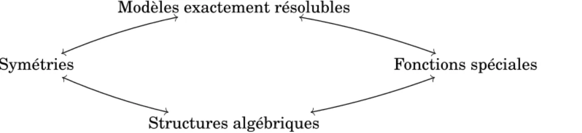
Liste des figures

1 Interactions entre les modèles exactement résolubles, les symétries,

les structures algébriques et les fonctions spéciales . . . 2 8.1 Uniform two-dimensional lattice of triangular shape . . . 217 9.1 Wavefunction amplitudes forξ = 0.8, ψ = 0.8, φ = π/4 and β = 15 . . . . 236 9.2 Wavefunction amplitudes forξ = 0.8, ψ = 0.8, φ = π/4 and β = 28 . . . . 237 9.3 Wavefunction amplitudes forξ = 0.5, ψ = 0.8, φ = π/4 and β = 15. . . . . 238 9.4 Wavefunction amplitudes forξ = 0.8, ψ = 0.8, φ = 0 and β = 15. . . . 239 28.1 Squeezing parameter Z_~n2

z for r = 2,4,6 (decreasing amplitudes) with

(28)

(29)

Remerciements

Mes premiers remerciements vont à Luc. Travailler sous sa supervision a été un grand privilège et même les mots les plus élogieux ne peuvent rendre justice à ses qualités de superviseur, tant au plan scientifique qu’au plan humain. Je remercie immensément mon père Christian à qui je dois beaucoup à la fois personnellement et professionnellement. Je remercie également ma mère Christine pour son éternel support à la fois fort et discret. Je remercie mes coauteurs, par ordre d’importance: Alexei Zhedanov, Hendrik De Bie, Mourad Ismail, Hiroshi Miki, Sarah Post et Guo-Fu Yu. Un merci très spécial à Casey. Un merci à Johanna, pour ses conseils et ses encouragements. Je veux aussi remercier chaleureusement tous les membres de ma famille et de ma belle famille; l’espace manque pour expliquer l’apport de chacun d’entre vous. Un remerciement final à mes amis, sur qui je peux toujours compter.

(30)

(31)

Introduction

L’étude des modèles exactement résolubles joue un rôle fondamental dans l’élaboration des théories qui visent à décrire et expliquer les phénomènes naturels. De manière générique, un modèle est dit exactement résoluble s’il est possible d’en exprimer mathé-matiquement les quantités d’intérêts de manière explicite. Cette notion prend des formes diverses selon le cadre de travail. Par exemple, en mécanique classique, on dira qu’un sys-tème formé de deux planètes en interaction gravitationnelle est exactement résoluble car on peut décrire de manière exacte les trajectoires suivies par chacun des corps [1]. En mé-canique quantique, le système formé d’un électron et d’un proton (atome d’hydrogène) est également considéré comme exactement résoluble puisque les énergies possibles du sys-tème et ses fonctions d’ondes sont explicitement connues, la notion de trajectoire ayant été évacuée [2]. La notion de résolubilité exacte n’est pas l’apanage de la physique théorique. Par exemple, en biologie mathématique, le modèle de Moran, qui décrit la dynamique d’une population de taille constante subissant des mutations aléatoires et dans laquelle deux types d’allèles se font compétition, est aussi vu comme exactement résoluble car on peut obtenir de manière explicite la loi de probabilité du nombre individus ayant un bagage génétique donné [3].

L’importance des modèles exactement résolubles en physique tient à de nombreux élé-ments; nous en mentionnons quelques-uns. Tout d’abord, ces modèles constituent un outil de choix dans la validation des principes théoriques fondamentaux. En effet, ils permet-tent de formuler des prévisions très précises qui peuvent être par la suite soumises à l’expérimentation. À ce titre, la description de la structure fine de l’atome d’hydrogène obtenue par le truchement de l’équation de Dirac est éloquente [4]. Ensuite, les mo-dèles ayant des solutions exactes permettent d’accéder à une compréhension plus fine du contenu physique des théories qui les sous-tendent car ils permettent l’analyse détaillée du rôle de tous les paramètres qui y interviennent; c’est d’ailleurs en partie pourquoi l’examen de ces systèmes occupe une place prépondérante dans les cursus de physique.

(32)

Un autre élément qui souligne l’importance des systèmes exactement résolubles est que ceux-ci sont constamment utilisés dans l’élaboration de modèles plus raffinés et dont les caractéristiques sont étudiées à partir de celles du modèle original, entre autres en uti-lisant la théorie des perturbations. On peut penser ici aux nombreux systèmes quantiques basés sur le modèle de l’oscillateur harmonique [2]. Finalement, l’étude des modèles ex-actement résolubles est un lieu de rencontre privilégié entre la physique théorique et les mathématiques. Ces deux disciplines se sont à de nombreuses reprises fertilisées mutuellement par le passé, conduisant à des avancées significatives dans les deux do-maines. Le théorème de Noether, qui relie les symétries aux lois de conservation en est un exemple particulièrement pertinent [5].

Les symétries sont le dénominateur commun des modèles exactement résolubles: em-piriquement, on observe qu’il n’y a de solutions exactes qu’en présence de symétries. Celles-ci se présentent sous diverses formes et sont décrites mathématiquement par des structures algébriques variées. Dans bien des cas, les solutions des modèles exacte-ment résolubles s’expriexacte-ment en termes de fonctions spéciales. Ces fonctions encodent les symétries des systèmes dans lesquels elles apparaissent. Un exemple typique est celui de l’oscillateur quantique en trois dimensions et des harmoniques sphériques. Ce système est invariant sous les rotations, décrites par le groupe SO(3). L’invariance sous les rota-tions conduit à la séparation de l’équation de Schrödinger en coordonnées sphériques, les harmoniques sphériques apparaissent comme solutions exactes à l’équation angulaire et elles forment une base pour les représentations irréductibles deso(3) [6].

La dynamique des modèles exactement résolubles, des symétries, des structures al-gébriques et des fonctions spéciales peut être inscrite dans le cercle vertueux suivant:

Modèles exactement résolubles

Symétriesvv 22 Fonctions spéciales)) ll Structures algébriquesrr 55 ++ hh

Figure 1: Interactions entre les modèles exactement résolubles, les symétries, les struc-tures algébriques et les fonctions spéciales

(33)

Le chemin typique que l’on songe parcourir dans ce schéma est le suivant. On imagine d’abord un modèle d’intérêt. Ensuite, on trouve les symétries de ce modèle et on détermine la structure mathématique qui décrit ces symétries. Puis, on construit les représentations de cette structure algébrique et on établit le lien entre ses représentations et les fonctions spéciales. Finalement on met à profit les fonctions spéciales pour exprimer les solutions du modèle et/ou pour en calculer certaines quantités importantes.

Il s’avère toutefois fructueux de prendre comme point de départ n’importe quel som-met de la figure 1. Par exemple, on peut obtenir et caractériser une nouvelle famille de fonctions spéciales, déterminer la structure algébrique dont ils encodent les propriétés, chercher des modèles dont les symétries sont décrites par cette structure et donner les solutions des modèles obtenus en termes de cette nouvelle famille de fonctions.

Le diagramme 1 reflète l’essence de la recherche qui a mené à la présente thèse, dans laquelle la résolubilité exacte est recherchée et étudiée par le truchement des symétries, des structures algébriques et de leurs représentations ainsi que des fonctions spéciales. La thèse comporte vingt-huit articles qui contribuent à un ou à plusieurs des axes de recherche qui apparaissent sur le diagramme 1. Les résultats originaux qu’elle contient sont en nombre. Ils concernent principalement les polynômes orthogonaux (une classe particulière de fonctions spéciales), les systèmes quantiques superintégrables (une classe de modèles exactement résolubles) et certaines algèbres et superalgèbres quadratiques telles que les algèbres de Bannai–Ito et de Racah.

La thèse se divise en cinq parties comprenant chacune une série d’articles sur un thème commun. Toutes les parties, à l’exception peut-être de la dernière, sont en fort lien les unes avec les autres via le diagramme 1. En outre, plusieurs articles auraient pu se retrouver dans une autre partie que celle où ils sont actuellement.

La partie I de la thèse est intitulée Polynômes orthogonaux multivariés et applications. Dans cette partie, on traite des interprétations physique et algébrique de six familles de fonctions orthogonales multivariées et on en détaille trois applications physiques. Dans l’introduction, on explique sommairement le contexte général de l’étude des polynômes orthogonaux multivariés. Dans les chapitres 1 à 3, on montre comment les familles de polynômes orthogonaux à d variables de Krawtchouk, Meixner et Charlier interviennent respectivement en tant qu’éléments de matrice des représentations unitaires des groupes de rotation SO(d + 1), du groupe de Lorentz SO(d,1) et du groupe euclidien E(d) sur les états de l’oscillateur harmonique [7, 8, 9]. On illustre de quelle façon cette interprétation conduit à une caractérisation complète de ces familles de polynômes. Dans le chapitre 4,

(34)

on établit une relation entre les polynômes de Krawtchouk à 2 variables, les coefficients de Clebsch-Gordan de l’algèbre su(1, 1) donnés par les polynômes de Hahn et les coeffi-cients de transition entre les bases sphérique et cartésienne de l’oscillateur harmonique en trois dimensions [10]. Dans le chapitre 5, on montre que les polynômes de Hahn à d variables de Karlin et McGregor interviennent dans les amplitudes de transition entre les états associés aux bases cartésienne et polysphérique de l’oscillateur singulier en d +1 dimensions [11]. On exploite ensuite cette identification pour donner une caractérisation complète de ces polynômes. Dans le chapitre 6, on utilise le lien entre le recouplage de n+1 représentations desu(1, 1) et le modèle superintégrable générique sur la n-sphère obtenu dans la partie IV pour étudier les coefficients 9 j desu(1, 1); on montre que ces coefficients sont donnés en termes de fonctions rationnelles orthogonales et on en extrait plusieurs propriétés [12]. Dans le chapitre 7, on met la table pour l’obtention d’une q-généralisation de la relation entre les polynômes de Krawtchouk multivariés et les représentations du groupe des rotations en déterminant le lien entre les polynômes de q-Krawtchouk et les « q-rotations » dans l’algèbre quantique Uq(sl2) [13]. Dans les chapitres 8 et 9, on présente

deux applications des polynômes orthogonaux multivariés. Premièrement, on explique comment les polynômes de Krawtchouk à deux variables peuvent être utilisés pour con-cevoir un réseau de spins à deux dimensions qui permet le transfert parfait d’états quan-tiques [14]. Deuxièmement, on élabore un modèle discret de l’oscillateur harmonique quantique en deux dimensions ayant la même algèbre de symétrie su(2) que le modèle usuel [15].

La partie II de la thèse est intitulée systèmes superintégrables avec réflexions. Dans cette partie, on étudie une série de systèmes quantiques superintégrables en deux et trois dimensions dont les hamiltoniens contiennent des opérateurs de réflexion de la forme R_if (xi) = f (−xi). Dans l’introduction, on rappelle la notion de superintégrabilité et on

définit les opérateurs de Dunkl. Dans les chapitres 10 et 11, on examine le modèle de l’oscillateur de Dunkl dans le plan [16, 17]. On montre que ce système est superinté-grable, on obtient ses constantes du mouvement et on en donne l’algèbre de symétrie et les solutions exactes. On montre que dans ce modèle les amplitudes de transition entre les états associés aux bases polaire et cartésienne sont exprimées en termes des coeffi-cients de Clebsch-Gordan de la superalgèbre de Lie osp(1|2) qui sont donnés en termes des polynômes duaux −1 de Hahn appartenant au tableau de Bannai–Ito discuté dans la partie III. On procède aussi à une analyse détaillée des représentations de l’algèbre de symétrie du modèle, dénommée algèbre de Schwinger–Dunkl. Dans le chapitre 12, on

(35)

considère une extension du modèle faisant intervenir des termes de potentiel singuliers; on montre que le système demeure superintégrable, on donne ses constantes du mouve-ment, son algèbre de symétrie et ses solutions exactes [18]. Dans le chapitre 13, on ex-amine l’oscillateur de Dunkl en trois dimensions, lui aussi superintégrable et exactement résoluble [19]. Dans le chapitre 14, on introduit le modèle superintégrable générique sur la 2-sphère avec réflexions [20]. Grâce aux résultats obtenus dans la partie IV, on montre que l’hamiltonien de ce système est lié à l’opérateur de Casimir total intervenant dans la combinaison de trois représentations irréductibles deosp(1|2). On détermine con-séquemment que l’algèbre de symétrie engendrée par les constantes du mouvement de ce système est l’algèbre de Bannai–Ito. On montre aussi la contraction de ce système vers l’oscillateur de Dunkl dans le plan. Finalement, dans le chapitre 15, on examine l’équation de Dirac–Dunkl sur la 2-sphère [21]. On montre que l’algèbre de symétrie de cette équation est aussi l’algèbre de Bannai–Ito, on construit les représentations de di-mension finie de cette algèbre et on construit les solutions exactes du modèle à l’aide de l’extension de Cauchy–Kovalevskaia.

La partie III s’intitule Tableau de Bannai–Ito et structure algébriques associées. Dans cette partie, on étudie des familles de polynômes orthogonaux appartenant à la classe des polynômes de Bannai–Ito et on étudie les structures algébriques associées à ces fonctions. Dans l’introduction, on rappelle l’origine des polynômes du tableau de Bannai–Ito, aussi appelés polynômes orthogonaux « −1 », et on explique brièvement la notion de bispectra-lité. Dans le chapitre 16, on démontre la bispectralité des polynômes complémentaires de Bannai–Ito, c’est-à-dire qu’on obtient l’opérateur duquel ils sont fonctions propres [22]. Dans le chapitre 17, on introduit et on caractérise une famille de polynômes « −1 » appelés polynômes de Chihara [23]. Dans le chapitre 18, on montre que les polynômes de Bannai– Ito interviennent comme coefficients de Racah de la superalgèbreosp(1|2), aussi appelée sl₋₁(2) [24]. Dans le chapitre 19, on obtient la structure algébrique qui sous-tend les polynômes duaux −1 de Hahn et on établit comment cette structure intervient dans le problème de Clebsch-Gordan de sl₋₁(2) [25]. Le chapitre 20 est le compte-rendu d’une conférence de revue sur l’algèbre de Bannai-Ito et ses applications [26]. Dans le chapitre 21, on introduit une q-généralisation des polynômes de Bannai–Ito et de leur algèbre en considérant les coefficients de Racah de la superalgèbre quantiqueosp_q(1|2) [27]. Dans le chapitre 22, on établit que la q-algèbre de Bannai–Ito est aussi l’algèbre de covariance de

osp_q(1|2) [28].

(36)

Dans cette partie, on détermine le lien entre le recouplage de représentations des algèbres

su(1, 1) et osp(1|2) et les systèmes superintégrables dont les constantes du mouvement sont du deuxième ordre. Dans l’introduction on rappelle les bases du problème de Racah, qui advient lors du recouplage de trois représentations. Dans le chapitre 23, on étudie les liens entre le problème de Racah pour l’algèbre de Lie su(1, 1), l’algèbre de Racah– Wilson et le système superintégrable générique sur la 2-sphère [29]. Dans le chapitre 24, on montre que l’algèbre de Racah peut également être vue comme l’algèbre de covariance quadratique de sl2 [30]. Le chapitre 25 est le compte-rendu d’une conférence de revue

sur l’algèbre de Racah [31]. Finalement, dans le chapitre 26, on établit le lien entre le problème de Racah pour la superalgèbre osp(1|2), l’algèbre de Bannai–Ito et le système superintégrable générique sur la 2-sphère avec réflexions [32].

La partie V est intitulée Polynômes multi-orthogonaux et applications. Elle est légère-ment à la marge des autres parties de la thèse et témoigne de mes premiers travaux. Dans l’introduction, la notion de d-orthogonalité et de multi-orthogonalité matricielle est re-vue. Dans le chapitre 27, on définit deux nouvelles familles de polynômes d-orthogonaux en utilisant les représentations de su(2) [33]. Dans le chapitre 28, on utilise ces résul-tats pour étudier les érésul-tats cohérents/comprimés de l’oscillateur fini et pour présenter de manière explicite une famille de polynômes multi-orthogonaux matriciels [34].

(37)

Partie I

Polynômes orthogonaux multivariés

et applications

(38)

(39)

Introduction

Les polynômes orthogonaux forment une classe particulièrement importante de fonctions spéciales [35], notamment en raison de leurs nombreuses applications à la physique mathématique, aux probabilités et aux processus stochastiques, à la théorie de l’approxi-mation et aux matrices aléatoires. Une suite de polynômes {Pn(x)}∞_n=0, où Pn(x) est un

polynôme de degré n en x, constitue une famille de polynômes orthogonaux s’il existe une fonctionnelle linéaireL telle que pour tous les entiers non-négatifs m et n, on a [36]

L [Pm(x)Pn(x)] = 0 si m 6= n et L [Pn(x)2] 6= 0.

De tous les polynômes orthogonaux, le sous-ensemble des polynômes orthogonaux hyper-géométriques est certainement l’un des plus importants [37]. Il est constitué des familles de polynômes orthogonaux qui peuvent s’écrire de manière explicite en termes de séries ou de q-séries hypergéométriques. Les séries hypergéométriques, dénotéespFq, sont définies

ainsi [35] pFq µ_a 1, a2, . . . , ap b₁, b2, . . . , bq ¯ ¯ ¯z ¶ =X k≥0 (a1, a2, . . . , ap)k (b1, b2, . . . , bq)k zk k!,

avec (a1, a2, . . . , ap)k= (a1)k(a2)k· · · (ap)koù (a)k est le symbole de Pochhammer

(a)k= k−1

Y

i=0

(a + i) avec (a)0= 1.

Les q-séries hypergéométriques, généralement dénotées parrφs, sont définies par [38] rφs µ_a 1, a2, . . . , ar b₁, b2, . . . , bs ¯ ¯ ¯q, z ¶ = X k≥0 (a1, a2, . . . , ar; q)k (b1, b2, . . . , bs; q)k(−1) (1+s−r)k_q(1+s−r)(k2) z k (q; q)k ,

avec (a1, a2, . . . , ar; q)k= (a1; q)k(a2; q)k· · · (ar; q)k où (a; q)k est le symbole de Pochhammer

q-déformé (a; q) =

k

Y

i=1

(40)

Les polynômes orthogonaux hypergéométriques sont typiquement organisés au sein d’une hiérarchie connue sous le nom de Tableau de Askey1[39]. Au sommet de cette hiérarchie trônent les polynômes de Askey–Wilson et les q-polynômes de Racah, qui ont chacun cinq paramètres, incluant q. Tous les polynômes du tableau d’Askey peuvent être obtenus à partir de ces deux familles par des limites, notamment la limite « classique » q → 1, ou alors par des choix particuliers de paramètres. Les polynômes du tableau d’Askey sont ubiquitaires, comme en témoignent les 1500 citations de la monographie de 1998 de Koekoek, Lesky et Swarttouw [39].

Les polynômes du tableau d’Askey ont presque tous une interprétation algébrique. Ils sont tantôt éléments de matrices ou vecteurs de base pour certaines représentations irré-ductibles d’algèbres de Lie de rang 1, tantôt coefficients de Clebsch-Gordan ou de Racah pour ces mêmes algèbres [40, 41, 42]. Dans tous les cas, les interprétations algébriques des familles de polynômes orthogonaux permettent d’en déduire un grand nombre de pro-priétés. En fait, le cadre algébrique est lui-même à l’origine de la découvert de certains de ces objets, dont les polynômes de Racah, q-Racah, Wilson et Askey–Wilson.

Il est naturel de chercher à généraliser la hiérarchie du tableau d’Askey aux poly-nômes orthogonaux multivariés. Il faut savoir toutefois que de manière générale, l’étude des polynômes orthogonaux à plusieurs variables est plus difficile que celle des polynômes univariés, notamment en raison du fait que dans le cas multivarié la mesure d’ortho-gonalité ne caractérise pas complètement les polynômes associés [43]. Il n’y pas à ce jour de théorie unifiée de tous les polynômes orthogonaux multivariés, à l’exception des polynômes multivariés associés aux systèmes de racines, qui ne sont pas étudiés dans cette thèse [43]. Cependant, nombreuses sont les familles qui sont connues et bien carac-térisées.

Les premiers exemples de familles de polynômes multivariés généralisant celles du tableau de Askey ont été proposés dans un cadre probabiliste au début des années 70. C’est Robert Griffiths qui a généralisé à plusieurs variables les familles de polynômes de Krawtchouk et de Meixner en utilisant des fonctions génératrices associées aux distri-butions multinomiale et multinomiale négative [44, 45]; voir aussi les travaux de Milch qui précèdent ceux de Griffiths [46]. Les polynômes multivariés de Krawtchouk étudiés par Griffiths ont par la suite été redécouverts à quelques reprises, notamment dans [47]. Durant la même période, Karlin et McGregor ont généralisé à plusieurs variables les polynômes de Hahn en considérant le modèle de Moran à plusieurs espèces [48]. On doit

(41)

aussi souligner les nombreux travaux de Koornwinder sur les polynômes à deux variables [49]. Plusieurs années plus tard, Tratnik a proposé une version multivariée du tableau d’Askey à q = 1 [50, 51]. Les polynômes multivariés proposés par Tratnik, qui incluent ceux de Karlin et McGregor, sont construits en combinant de manière non triviale des polynômes orthogonaux univariés du tableau d’Askey. De nombreux travaux visant la caractérisation de ces polynômes ont par la suite été publiés [52]. Plus récemment, la même approche a été reprise par Gasper et Rahman pour définir des q-déformations des polynômes proposées par Tratnik [53]; ces familles demeurent toutefois relativement peu étudiées [54].

Cette partie de la thèse porte sur l’interprétation physique et algébrique de certaines familles de polynômes orthogonaux ainsi que sur certaines de leurs applications concrètes à la physique. Tout d’abord, on montre que les polynômes de Krawtchouk, de Meixner (tels que définis par Griffiths) et de Charlier à d-variables correspondent aux éléments de matrices des représentations unitaires des groupes de Lie SO(d + 1), SO(d,1) et E(d) sur les états de l’oscillateur harmonique. Les résultats qui concernent les groupes SO(d + 1) et E(d) sont directement liés aux propriétés de transformation de systèmes d’oscillateurs harmoniques sous les rotations et les transformations euclidiennes. On illustre également le lien entre les polynômes de Krawtchouk à deux variables et les coefficients de tran-sition entre les états des bases cartésienne et sphérique pour l’oscillateur harmonique en trois dimensions. On montre aussi que les polynômes de Hahn à d variables de Karlin et McGregor interviennent dans les amplitudes de transition entre les états des bases cartésienne et polysphérique de l’oscillateur singulier en d + 1 dimensions. On exa-mine également les coefficients 9 j desu(1, 1) par la lorgnette du système superintégrable générique sur la 3-sphère et on montre que ces coefficients s’expriment non pas en ter-mes de polynôter-mes, mais en terter-mes de fonctions rationnelles. Par ailleurs, on montre que les polynômes de q-Krawtchouk interviennent en tant qu’éléments de matrice des « q-rotations » de l’algèbre quantique Uq(sl2). Les deux applications qui sont présentées

concernent respectivement le transfert parfait d’états quantiques à l’aide de réseaux de spins et la discrétisation du modèle de l’oscillateur quantique en deux dimensions.

(42)

(43)

Chapitre 1

The multivariate Krawtchouk

polynomials as matrix elements of the

rotation group representations on

oscillator states

V. X. Genest, L. Vinet et A. Zhedanov (2013). The multivariate Krawtchouk polynomials as matrix elements of the rotation group representations on oscillator states. Journal of Physics A: Mathematical and Theoretical 46 505203

Abstract. An algebraic interpretation of the bivariate Krawtchouk polynomials is

pro-vided in the framework of the 3-dimensional isotropic harmonic oscillator model. These polynomials in two discrete variables are shown to arise as matrix elements of unitary reducible representations of the rotation group in 3 dimensions. Many of their properties are derived by exploiting the group-theoretic setting. The bivariate Tratnik polynomials of Krawtchouk type are seen to be special cases of the general polynomials that corre-spond to particular rotations involving only two parameters. It is explained how the approach generalizes naturally to (d + 1) dimensions and allows to interpret multivariate Krawtchouk polynomials as matrix elements of SO(d + 1) unitary representations. Indi-cations are given on the connection with other algebraic models for these polynomials.

(44)

1.1 Introduction

The main objective of this article is to offer a group-theoretic interpretation of the mul-tivariable generalization of the Krawtchouk polynomials and to show how their theory naturally unfolds from this picture. We shall use as framework the space of states of the quantum harmonic oscillator in d + 1 dimensions. It will be seen that the Krawtchouk polynomials in d variables arise as matrix elements of the reducible unitary representa-tions of the rotation group SO(d + 1) on the energy eigenspaces of the (d + 1)-dimensional oscillator. For simplicity, we shall focus on the d = 2 case. The bivariate Krawtchouk poly-nomials will thus appear as matrix elements of SO(3) representations; we will indicate towards the end of the paper how the results directly generalize to an arbitrary finite number of variables.

The ordinary Krawtchouk polynomials in one discrete variable have been obtained by Krawtchouk [19] in 1929 as polynomials orthogonal with respect to the binomial distribu-tion. They possess many remarkable properties [17, 25] (second-order difference equation, duality, explicit expression in terms of Gauss hypergeometric function, etc.) and enjoy numerous applications. The importance of these polynomials in mathematical physics is due, to a large extent, to the fact that the matrix elements of SU(2) irreducible repre-sentations known as the Wigner D functions can be expressed in terms of Krawtchouk polynomials [4, 18].

The determination of the multivariable Krawtchouk polynomials goes back at least to 1971 when Griffiths obtained [5] polynomials in several variables that are orthogonal with respect to the multinomial distribution using, in particular, a generating function method. These polynomials, especially the bivariate ones, were subsequently rediscov-ered by several authors. For instance, the 2-variable Krawtchouk polynomials appear as matrix elements of U(3) group representations in [26] and the same polynomials occur as 9 j symbols of the oscillator algebra in [29]. An explicit expression in terms of Gel’fand-Aomoto generalized hypergeometric series is given in [24]. Interest was sparked in recent years with the publication by Hoare and Rahman of a paper [11] in which the 2-variable Krawtchouk polynomials were presented, anew, from a probabilistic perspective. This led to bivariate Krawtchouk polynomials being sometimes called Rahman polynomials. A number of papers followed [6, 7, 8, 23]; the approach of [11], related to Markov chains, was extended to the multivariate case in reference [7] to which the reader is directed for an account of the developments at that point in time.

(45)

Germane to the present paper are references [13] and [12]. In the first of these pa-pers, Iliev and Terwilliger offer a Lie-algebraic interpretation of the bivariate Krawtchouk polynomials using the algebra sl3(C). In the second paper, this study was extended by

Iliev to the multivariate case by connecting the Krawtchouk polynomials in d variables to sl_d+1(C). In these two papers, the Krawtchouk polynomials appear as overlap coef-ficients between basis elements for two modules of sl3(C) or sld+1(C) in general. The

basis elements for the representation spaces are defined as eigenvectors of two Cartan subalgebras related by an anti-automorphism specified by the parameters of the poly-nomials. The interpretation presented here is in a similar spirit. We shall indicate in Section 5 and in the appendix what are the main observations that are required if one wishes to establish the correspondence. In essence, the key is in the recognition that the anti-automorphism used in [12] and [13] can be taken to be a rotation (times i). The anal-ysis is then brought in the realm of the theory of Lie group representations. This entails connecting two parametrizations of the polynomials: the one used in the cited literature and the other that naturally emerges in the interpretation to be presented, in terms of rotation matrix elements. It is noted that the connection with SO(d + 1) rotations readily explains the d(d + 1)/2 parameters of the polynomials.

A major advance in the theory of multivariable orthogonal polynomials was made by Tratnik [27], who defined a family of multivariate Racah polynomials, thereby obtaining a generalization to many variables of the discrete polynomials at the top of the Askey scheme and extending the multivariate Hahn polynomials introduced by Karlin and Mc-Gregor in [16] in the context of linear growth models with many types. These Racah polynomials in d variables depend on d + 2 parameters; they can be expressed as prod-ucts of single variable Racah polynomials with the parameter arguments depending on the variables. Using limits and specializations, Tratnik further identified multivariate analogs to the various discrete families of the Askey tableau, thus recovering the mul-tidimensional Hahn polynomials of Karlin and McGregor and obtaining in particular an ensemble of Krawtchouk polynomials in d variables depending on only d parameters (in contrast to the d(d + 1)/2 parameters that we were so far discussing). We shall call these the Krawtchouk-Tratnik polynomials so as to distinguish them from the ones introduced by Griffiths. The bispectral properties of the multivariable Racah-Wilson polynomials defined by Tratnik have been determined in [3]. As a matter of fact, the Krawtchouk-Tratnik polynomials are also orthogonal with respect to the multinomial distribution and have been used in multi-dimensional birth and death processes [22]. It is a natural

(46)

ques-tion then to ask what relaques-tion do the Krawtchouk-Tratnik polynomials have with the other family. As will be seen, the former are special cases of the latter corresponding to particular choices of the rotation matrix. This fact had been obscured it seems, by the usual parametrization which is singular in the Tratnik case.

To sum up, we shall see that the multivariable Krawtchouk polynomials are basically the overlap coefficients between the eigenstates of the isotropic harmonic oscillator states in two different Cartesian coordinate systems related to one another by an arbitrary rota-tion. This will provide a cogent underpinning for the characterization of these functions: simple derivations of known formulas will be given and new identities will come to the fore.

In view of their naturalness, their numerous special properties and especially their connection to the rotation groups, it is to be expected that the multivariable Krawtchouk polynomials will intervene in various additional physical contexts. Let us mention for example two situations where this is so. The bivariate Krawtchouk polynomials have already been shown in [20] to provide the exact solution of the 1-excitation dynamics of a two-dimensional spin lattice with non-homogeneous nearest-neighbor couplings. This allowed for an analysis of quantum state transfer in triangular domains of the plane. The multivariate Krawtchouk polynomials also proved central in the construction [21] of superintegrable finite models of the harmonic oscillator where they arise in the wavefunc-tions. Let us stress that in this case we have a variant of the relation with group theory as the polynomials are basis vectors for representation spaces of the symmetry group in this application. Indeed, the energy eigenstates of the finite oscillator in d dimensions are given by wavefunctions where the polynomials in the d discrete coordinates have fixed total degrees. This is to say that the Krawtchouk polynomials in d variables, with given degree, span irreducible modules of SU(d).

The paper is structured as follows. In Section 2, we specify the representations of SO(3) on the energy eigensubspaces of the three-dimensional isotropic harmonic oscil-lator. In Section 3, we show that the matrix elements of these representations define orthogonal polynomials in two discrete variables that are orthogonal with respect to the trinomial distribution. In Section 4, we use the unitarity of the representations to derive the duality property of the polynomials. A generating function is obtained in Section 5 using boson calculus and is identified with that of the multivariate Krawtchouk polynomi-als. The recurrence relations and difference equations are obtained in section 6. An inte-gral representation of the bivariate Krawtchouk polynomials is given in terms of Hermite