A numerical reduced model for thin liquid films sheared by a gas flow

O

pen

A

rchive

T

OULOUSE

A

rchive

O

uverte (

OATAO

)

OATAO is an open access repository that collects the work of Toulouse researchers and

makes it freely available over the web where possible.

This is an author-deposited version published in :

http://oatao.univ-toulouse.fr/

Eprints ID : 18393

To link to this article : DOI:

10.1016/j.jcp.2015.08.018

URL :

http://dx.doi.org/10.1016/j.jcp.2015.08.018

To cite this version :

Lavalle, Gianluca and Vila, Jean-Paul and

Blanchard, G. and Laurent, Claire and Charru, François A numerical

reduced model for thin liquid films sheared by a gas flow. (2015)

Journal of Computational Physics, vol. 301. pp. 119-140. ISSN

0021-9991

Any correspondence concerning this service should be sent to the repository

administrator:

staff-oatao@listes-diff.inp-toulouse.fr

A

numerical

reduced

model

for

thin

liquid

films

sheared

by

a

gas

flow

G. Lavalle

a

,

∗

_,

_{J.-P. Vila}

a

,

b

_,

_{G. Blanchard}

a

_,

_{C. Laurent}

a

_,

_{F. Charru}

c a_{ONERA,AerodynamicsandEnergeticsModelingDepartment,31055Toulouse,France}

b_{InstitutdeMathématiquesdeToulouse,INSA,GMM,31055Toulouse,France}

c_{InstitutdeMécaniquedesFluidesdeToulouse,CNRS-UniversitédeToulouse,31400Toulouse,France}

a

b

s

t

r

a

c

t

Keywords: Thinfilms Gasflows Interfacialflows Movingmesh Low-Mach Long-wavemodel

Thenon-lineardynamicsofthin liquidfilmsshearedbyalaminargasflowinachannel is investigated. Such a two-layer flow is driven by pressure gradient and possibly by the gravity force. We describe the liquidphase with along-wave integral model, with the aimto savecomputationalcostwithrespecttothe fullDirectNumerical Simulation (DNS)oftheNavier–Stokesequations.Wederivethislong-wavemodelbytheintegration ofthe Navier–Stokesequations overthe filmthickness,and byanasymptoticexpansion up to the first order in terms of a long-wave parameter. These depth-integrated (or shallowwater)equationsare discretizedbymeansofanaugmentedsystem,whichholds an evolution equation for the surfacetension in order to avoid numerical instabilities of classical upwind and centered schemes. On the otherside, westudy the gas phase with compressibleNavier–Stokes equations,and wediscretizethem bymeansofa low-Mach scheme, accounting also for moving meshes (ALE). In order to analyze liquid– gas interactions, we introduce then a coupling methodology between depth-integrated equations andNavier–Stokesequations.Thisapproachrepresentsacompromisebetween the two existing methods: thefull DNS,and the full long-wave model appliedto both phases. Inordertovalidatethisapproach,wepresentcomparisonswithDNS,showinga good agreementofspatio-temporalevolutionsofthe filmthicknessandthe stressfield. Furthermore,interfacialshearstressandpressuregradientevolutionsareshowntobein accordancewiththoseprovidedbytwo-layersecond-orderlow-dimensionalmodels.

1. Introduction

Thin liquid films sheared by a laminar gas flow are often encountered in several industrial processes, such as heat and masstransfers inheat pipes, evaporatorsanddistillation columns.Meanwhile, two-layer flows mightalso be found in the aerospace domain, where the gas is meanly turbulent: pre-filming for injection systems, water ingestion within turboengines,de-icingofaircraftsystems,depositionofaluminafilmsoverthewallsofsolidrocketmotors.

Becauseofthedevelopmentofsurface waves,thedeformableinterfaceplaysarelevantroleintheinteractionbetween thetwophases.Indeed,experiments[1,2]haveprovedthattheoccurrenceofwavesattheinterfaceconsiderablyamplifies

*

Correspondingauthor.

E-mailaddresses:gianluca.lavalle@gmail.com(G. Lavalle),vila@insa-toulouse.fr(J.-P. Vila),ghislain.blanchard@math.univ-toulouse.fr(G. Blanchard),

claire.laurent@onera.fr (C. Laurent),charru@imft.fr (F. Charru).

the transfers between the liquid and the gas. Given that these problems are of high complexity, numerical simulations turnto be usefulforengineeringinvestigations. There exist several worksaboutDNS appliedto film–gasdynamics, that is to say performedby usingthe Navier–Stokes equations for both the phases. Concerning liquid films in a passive gas atmosphere,werecallthestudiesofSalamonetal.[3]andTrifonov[4],aswellasRamaswamyetal.[5],whohavecoupled afinite-element approachwiththe ArbitraryLagrangian Eulerian(ALE) method tostudytemporalandspatial stability of non-linearwaves;fortwo-layerco-currentflows,themainworksarethoseofLietal.[6],Zhangetal.[7]andFrank[8,9],as wellasDietze&Ruyer-Quil[10]withGerris(Popinet[11])andOpenFOAMflowsolvers,whileTrifonov[12]hasinvestigated counter-currentflows.

However,experiments[13–17]haveshownthatthewavesdevelopingongravity-drivenliquidfilms,orattheliquid–gas interface for channel flows, are much longer than the film thickness. Thissuggests the introduction of low-dimensional modelsbuiltonafilmparameter

ε

=

h

/λ

<<

1 whichmeasuresthesmallnessofthefilmthicknesscomparedtothe wave-length of interfacial waves. Furthermore,the development of low-dimensional models to describe the dynamics of film flows andtwo-layer flows ingeneral, helps decrease thecomputational cost with respect to DNS, particularlyexpensive whenanalyzingtheindustrialconfigurations,suchasthosepreviouslycited.

ThesereducedmodelsaremostlybasedontheearliestworksofBenney[18]andShkadov[19]forfallingfilmsdownan inclinedplane.Benney[18]hasdevelopedasymptoticsolutionsforlong-wavedisturbancesofliquidfilmssubjecttogravity. However, the resulting evolution equation fails when studying the behavior ofan unstable film far fromthe instability threshold. On the other hand, Shkadov [19] has developed an integral model of the boundary–layer equations. Despite thismodel ensures tocapture thelong-wave interfacial instabilities,it doesnot assure theright stability threshold.This shortcominghasbeenthen addressedby Ruyer-Quil&Manneville[20,21],by addingcorrectionsoffurtherorders in

_ε

to thevelocityprofilewithintheliquidfilm.

Inarecentwork,Dietze&Ruyer-Quil[10]havedevelopedafullyreducedmodelforconfinedtwo-layerflows,extending theweighted residualboundary–layertechnique(WRIBL)[21]totwophases.Thismodelallowstogetridoftheweakness ofpreviousworksinvolvingthemodelization oftwo-layerflows[22–25],whicharebasedontheabovementionedstudies ofBenneyandShkadov.Nevertheless,theuseofintegralequationsforthegasphaserestrictsthefieldofapplicationofsuch amodelbecausethethicknessofthegasflowmustbemuchsmallerthanthewavelengthofinterfacialwaves.

Meanwhile,the WRIBLapproach hasbeenalsoemployed by Tseluiko & Kalliadasis [26] tomodel liquidfilms sheared by a counter-current turbulent gas flow. However, given the high gas speed, they have legitimately neglected the film velocity,which inturnbecomesessential withcomparablefilm–gasvelocities,such asthescenarios treatedinthiswork. Subsequently,Vellingirietal.[27]haveusedthesamemethodologytostudyco-currentflowsinsideachannel.

Therefore,inthispaperweintroduceanewmodelfortwo-layerchannelflows,withtheaimtoovercometherestrictions ofthepreviouslycitedworks.Wecouplealow-dimensionalmodelfortheliquidphasetocompressibleNavier–Stokes equa-tionsaccountingforthegasphase.Thismethodology,thatwecallSWANS(ShallowWaterALENavier–Stokes),isbasedon themovingmeshtechnique(ALE)andcanbethenintegratedinsideindustrialcodes,suchastheCEDREplatform [28] de-velopedatONERA.ThisrepresentsthemainreasonforhavingchosentosolveflowsatlowMachnumberwithcompressible schemes.

Whencompared tothe previouslycited works, ourmodelprovides thefollowing advantages:thegasthicknessis not restrictedby thelong-wave theory,permitting tostudynumerous industrialapplications; theuseofNavier–Stokes equa-tionsforthegasphaseallowsustohaveawidedescriptionofthegasfields,namelyvelocity,shearstressandpressure;the methodologyof couplingshallow watermodel to Navier–Stokesequations representsan intermediate approachbetween the resolutions typically used fortwo-layer flows, that are eitherthe fully Navier–Stokes orthe fully shallowwater ap-proaches;thelow-dimensionalmodelusedfortheliquidphaseallows reducingthecomputationalcostcomparedtoDNS. Furthermore,theuseoftheALEmethodrepresentsanoriginalityinthecouplingprocess:sofarithasbeenappliedonly togravity-driven falling filmortwo-phase Navier–Stokesequations(Hirt etal.[29], Chan[30],Pracht [31],Soulaïmaniet al.[32]andRamaswamyetal.[5]).OriginalfromacomputationalpointofviewisalsothecombinationoftheALEtechnique andthelow-Machscheme.

Thearticleisstructuredasfollows:thephysicalproblemisdiscussedinSection2;thelong-wavefilmmodelisdescribed andderived in Section 3; Section 4 showsthe coupling strategy betweenthe long-wave film model and Navier–Stokes equationsaccountingforthegasphase; Section5 describesthe computationalapproachforthe liquidphaseandthegas phase,aswellasthecouplingbetweenthetwo;Section6showstwotest-casesandthemainresults;Section7gathersthe conclusionsofthiswork.

2. Thegeneralframework

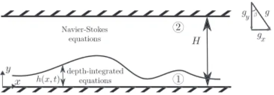
Theproblemconsideredherebyisatwo-layerchannelflow,assketchedinFig. 1.Thedomainistwo-dimensional:athin liquidfilmonthelowerwallofthechannelisshearedbyalaminargasflowonthetopofit.Thetwo-layerflowisdriven bypressuregradientandpossiblybythegravityforce,throughtheinclination

β

ofthechannel.WithreferencetoFig. 1,H

denotestheheight ofthechannel, andh the localthicknessoftheliquidfilm.Subscripts1 and2 refer toliquidandgas phases,respectively.

Withthisarticle,ouraimistodevelopacouplingmethodologybetweendepth-integratedequationsandNavier–Stokes equations,accountingforliquidandgasphases, respectively. Bymeansofthiscoupling technique,we wantto studythe

Fig. 1. Sketch of the two-layer channel flow: index 1 refers to the liquid film, while index 2 to the gas phase.

Fig. 2. Sketch of a liquid film subject to gravity and to interfacial shear stress and pressure.

non-linear wave dynamics at the interface between the two phases. We first study the liquid problem, and develop a low-dimensionalmodelforthinliquidfilmsshearedbyagasflow,bymeansofthelong-wavetheory.Thismodelisaccurate at order one in

ε

: it predicts the right linear stability threshold of long waves andis valid in the limit

ε

Re

<<

1. In addition,asshownlater,space–timethicknessvariationsoftheliquidfilmareassumedtobesmall,whilenoassumptionis requiredabouttheamplitudeofthethicknessitself.Subsequently,wepresenthowtocouplethismodeltotheNavier–Stokes equationsinthegasphase.

3. Liquidfilmmodeling

WithreferencetoFig. 2,thegoverningequationsforliquidfilmsdownaninclinedplaneandsubjecttogiveninterfacial shearstress

τ

˜

i

(

x

˜

,

˜

t

)

andpressure p

˜

i

(

x

˜

,

˜

t

),

aretheincompressibleNavier–Stokesequations:

ρ

(∂

tu

˜

+ ˜

u

· ∇ ˜

u

)

= −∇ ˜

p

+

ρ

g

+

µ

∇

2u

˜

,

∇ · ˜

u

=

0

.

(1)

Here the tilde designates dimensional variables,

_∇

the nabla operator, u

_˜

= ( ˜

u

,

v

˜

)

is the film velocity with stream-wise (x)

˜

andcross-stream(

˜

y)components, p the

˜

pressure,g

_{= (}

g sin

β,

−

g cos

β)

thegravityforce, and

ν

=

µ

/

ρ

thekinematic viscosityoftheliquid.

Atthebottom,wherey

_˜

₌

0,theno-slipconditionreads

˜

u

₌

0

,

v

˜

₌

0

.

(2)

Atthefilmsurfaceinstead,wherey

˜

_{= ˜}

h,boundaryconditionsstatethecontinuityoftangentialandnormalstresses,namely

˜

t

_{· ˜}

T(˜n)

_{= ˜}

τ

i

(˜

x

,

t

˜

) ,

(3)

˜

n

_{· ˜}

T(˜n)

_{= ˜}

pi

(˜

x

,

˜

t

)

+

γ

∇ · ˜

n

,

(4)

where

˜

t and n are

˜

thetangent andoutward normal unit vectorstothe interface, T

˜

(˜n)

_{= ˜}

₆

_{· ˜}

_{n is the stress vectorat the}

interface, while

6

˜

is the stress tensor, and

γ

the surface tension. The conditionsat the interface are completed by the kinematiccondition,whichimposestheinterfacetobeamaterialline,andreads

∂

th

˜

+ ˜

u

|

h

∂

xh

˜

= ˜

v

|

h

.

(5)

The system of equations(1) withthe corresponding boundary conditions (2)–(5) entirely describesthe dynamics of the liquidfilmofFig. 2.

Inordertoidentifythedominanttermsofthesystem(1),weworkwithdimensionlessequationsbymeansof dimen-sionlessvariablesrepresentativeoftheliquidflow,suchas

x

₌

˜

x

˜

h0

,

y

₌

y

˜

˜

h0

,

t

₌

˜

t

˜

h0/ ˜U0

,

(6a) u

₌

u

˜

˜

U0

,

v

₌

v

˜

˜

U0

,

p

₌

p

˜

ρ

U

˜

2₀

,

τ

i

=

˜

τ

i

˜

U0

µ

/ ˜

h0

.

(6b)

Here, h

˜

0 is the film thickness and U

˜

0 the average velocity of the uniformflow (alternatively,other quantities mightbe chosenascharacteristicscales).

Furthermore, asalready mentioned, waves that develop on the surface of a liquidfilm atmoderate Re are generally longcomparedtothefilmthickness. Therefore,thefilmparameter

ε

<<

1 scalesspaceandtimederivatives

∂

x,t (withthe

exceptionof

∂

xp givento thepressurescaling), revealingthatno assumptionmustbe consideredabouttheamplitudeof

thethicknessitself.

Asamatteroffact,for

ε

Re

<<

1 thegoverningequations(1)upto

O(

ε

)

reduce totheboundary–layerequations.Their dimensionlessformreads























∂

xu

+ ∂

yv

=

0

∂

tu

+

u

∂

xu

+

v

∂

yu

= −∂

xp

+

1 Frsin

β

+

1 Re

∂

y yu 0

_{= −}

1 Frcos

β

− ∂

yp

,

(7)

wheretheReynoldsandFroudenumbersaredefinedas

Re

₌

U

˜

0

h

˜

0

ν

,

Fr

=

˜

U

₀2

g

h

˜

0

.

(8)

Thecorrespondingboundaryconditions(2)atthewall,wherey

₌

0,are

u

₌

0

,

v

₌

0

.

(9)

Attheinterface,wherey

₌

h,thecontinuityoftangentialandnormalstresses(3)–(4),aswellasthekinematiccondition(5), becomerespectively p

_|

h

=

pi

(

x

,

t

)

−

1 We

∂

xxh

,

(10a)

∂

yu

|

h

=

τ

i

(

x

,

t

) ,

(10b)

∂

th

+

u

|

h

∂

xh

=

v

|

h

,

(10c)

whereWe

₌

ρ

U

˜

2₀h

˜

0γ−1 _{istheWebernumber.Thesystemofequations(7)completedbyboundaryconditions(9)and(10)} representsthefulldimensionlessboundary–layersystemoftheproblemofFig. 2.

3.1. Integrationoverthefilmthickness

As already mentioned, we use a long-wave integral model to study the liquid film: the integration of the equations allowsustoreducethedegreesoffreedomofthesystemandpassfromunknownsu,v and p totheaverage filmthickness

h andflowrateq.However,beforeintegratingtheboundary–layerequations(7),itissuitabletoreplacethey-momentum equationintothe x-momentumthrough thepressure p.Thiscan beachievedbyintegratingthethird ofthe (7)withthe boundarycondition(10a),whichleadstothehydrostaticpressurefield

p

(

x

,

y

,

t

)

= −

x

Z

0 G

(

x

)

dx

₋

1 We

∂

xxh

+

1 Frcos

β(

h

−

y

) .

(11)

Withreferencetotheequation(10a),

₋

G

(

x

)

istheinterfacialpressuregradient

∂

xpiinthegas(alternatively,onecanchoose

thepressuregradientatthebottom).Thus,boundary–layerequations(7)reducetoasystemoftwoequations,whichreads







∂

xu

+ ∂

yv

=

0

∂

tu

+

u

∂

xu

+

v

∂

yu

=

G

−

cos

β

Fr

∂

xh

+

sin

β

Fr

+

1 Re

∂

y yu

+

1 We

∂3x

h

.

(12)

TheintegrationoftheseequationsoverthefilmthicknessisperformedbythehelpoftheLeibniz’sintegrationruleandthe boundarycondition(10c).Wefindthesystem

∂

th

+ ∂

xq

=

0

,

(13a)

∂

tq

+ ∂

x

³

Z

h 0 u2dy

´

₊

cos

β

Fr h

∂

xh

=

1 Re

³

3

h

₊

τ

i

− ∂

yu

|

0

´

+

_We1 h

∂3x

h

,

(13b)

whereq

₌

R

₀hudy istheflowrate,

τ

w

= ∂

yu

|

0 thewallshearstressand

3

=

Re_Frsin

β

+

Re G

(

x

)

(14)

Theseequationscouplethefilmthicknessh andtheflowrateq (alternatively,y-averagedstream-wisevelocityU

₌

q

/

h),

withthe exception ofthe integral ofsquared velocity andthewall shear stress. Hence,integrated boundary–layer equa-tions(13)needclosuremodels.Inordertoclosetheseequations,weprovideanasymptoticexpansionoftheboundary–layer equations(12)withrespecttothesmallparameter

ε

,andthusobtainvelocityandstressfieldsat

O(

ε

).

Recallingthat

∂

x,t

∼

ε

andv

<<

u,thevelocityfieldcanbeexpandedas

u

(

x

,

y

,

t

)

=

u(0)

₍

_x

_,

_y

_,

_t

₎

₊

_u(1)

₍

_x

_,

_y

_,

_t

₎

_{+ . . . ,}

_(15a)

v

(

x

,

y

,

t

)

₌

v(1)

(

x

,

y

,

t

)

₊

v(2)

(

x

,

y

,

t

)

_{+ . . . ,}

(15b) where thesuperscript

(0)

denotestheleading-order (parallel)flow and

(1)

denotes order

_ε

corrections. Bydoingso, the momentumequationofthesystem(12)attheleadingordersimplyreads

3

+ ∂

y yu(0)

=

0,where

3

isdefinedin(14).The

resultingdoubleintegrationprovides

u(0)

₍

_x

_,

_y

_,

_t

₎

₌

_τ

iy

+ 3

¡

hy

−

y2 2

¢

,

(16)

thankstotheboundaryconditions(10b)and(9).Thecorrespondingflowratereads

q(0)

₌

1 3

3

h

3

+

1₂

τ

ih2

.

(17)

Thewallshearstressinsteadis

τ

w(0)

=

3

q(0)

h2

−

1

2

τ

i

.

(18)

Inaddition,thecross-streamvelocityisgivenbythecontinuityequation

∂

xu

+ ∂

yv

=

0,as

v(1)

₌

Re

∂

xG

y3

6

− (∂

x

τ

i

+ 3∂

xh

+

Re

∂

xG h

)

y2

2

.

(19)

Finally,at

O(

ε

),

themomentumequationof(12)becomes

∂

tu(0)

+

u(0)

∂

xu(0)

+

v(1)

∂

yu(0)

=

1 We

∂3x

h

−

cos

β

Fr

∂

xh

+

1 Re

∂

y yu (1)

_,

₍₂₀₎

whosedoubleintegrationgivesthevelocityprofileatorderone,namely

u(₁1)

₌

Re 24

(

2h

−

y

)(

−

y 2

+

2hy

₊

4h2

)

y

"

¡

3

h

₊

τ

i

¢

3 ∂

xh

−

Re

∂

tG

#

+

Re 2 360

"

3(

y5

₊

24h5

₊

15h2y3

₋

6hy4

₋

20h3y2

)

₊

3

τ

i

(

−

10h4

+

5hy3

−

2y4

)

#

y

∂

xG

+

Re₂₄

"

(

4h3

₋

y3

)

τ

i

+ (

2h3

+

y3

−

2hy2

)3

h

#

y

∂

x

τ

i

−

Re 6

(

3h 2

−

y2

)

y

∂

t

τ

i

+

Re₂

³

_We1

∂3x

h

₋

cos

β

Fr

∂

xh

´

(

2h

₋

y

)

y

.

(21)

Thefirst-orderwallshearstress

τ

w(1)

= ∂

yu(1)

|

0 insteadreads

τ

w(1)

=

1 3

3

h 3_Re

₍₃

_h

+

τ

i

) ∂

xh

+

1 60Re 2_h4

₍

₄

₃

_h

−

5

τ

i

) ∂

xG

+

₁₂1 Re h3¡

3

h

₋

2

τ

i

¢

∂

x

τ

i

−

1 3Re 2_h3

∂

tG

−

1 2Re h 2

∂

t

τ

i

.

(22)

Oncevelocityandstressfieldshavebeenfullycomputed,system(13)ofintegratedboundary–layerequationscanbefinally closed.However,giventothesmallinertialeffectsconsideredintheliquid(thel.h.s.of(13b)isat

O(

ε

)),

onlythewallshear stress termneeds a closurelawat orderone, whereas theintegral ofsquared velocityrequires simplythe leading-order parabolicprofile(16)(Ruyer-Quil&Manneville[20,21],Luchini&Charru[33,34],Kalliadasisetal.[35]).

Therefore,byreplacingthevelocityprofile(16)intotheintegralofsquaredvelocityappearingin(13b),andbyusingthe wallshearstress(18)and(22),equations(13)read

∂

th

+ ∂

xq

=

0

,

(23a)

∂

tq

+ ∂

x

h

₆ 5 q2 h

+

1 60h 3

τ

i

(3

h

+

2

τ

i

)

i

+

cos_Fr

β

h

∂

xh

=

1 Re

h

3

h

₊

τ

i

−

τ

w

i

+

_We1 h

∂3x

h

,

(23b) where

_τ

w

=

τ

w(0)

+

τ

w(1),givenby(18)and(22).Onecannoticethattheclosureoftheintegralofsquaredvelocityfollows

thegravity-drivenfilmmodeling(Shkadov[19]),accordingtowhich

R

₀hu2dy

₌

6/5q2_h−1_{.However,forshearedliquidfilms,} theanalysisinvolvesanadditionaltermaccountingfor

τ

i.

4. Two-layerflowandliquid–gasboundaryconditions

Recallingthatsubscripts1,2 refertothefilmandthegas,respectively,wedevelophereacouplingmethodologybetween thetwophases,inordertostudythetwo-layerproblemofFig. 1.Beforeperformingthecoupling,wewritethesystem(23)

inan another form: we move the

∂

xh termofthe wall shear stress correction (22)fromthe r.h.s. to the l.h.s.of(23b);

also,wereplace1/5q2

_/

_{h oftheinertialtermsin(23b)byusingtheleading-orderflowrate(17),whichisvalidbecausethe} l.h.s.is

O(

ε

).

Inadditiontofulfill theGalileaninvariance(Lavalleetal.[36]),thisnewformkeepsthesamepropertiesof consistencyas(23)andallowsustousethetechniqueoftheaugmentedsystemforthediscrete form,tobe shownlater. Theseequationsthusread(Lavalle[37])

∂

th

+ ∂

xq

=

0

,

(24a)

∂

tq

+ ∂

x

³

q2 h

+

P

´

=

_Re1

h

3

h

₋

3q h2

+

3 2

τ

i

−

T

i

+

_We1 h

∂3x

h

,

(24b)

where P isthe“pressure”part(inanalogywiththeNavier–Stokesequations)oftheshallowwatermomentumfluxandT

derivesfromthefirst-orderwallshearstress(22):

P

₌

2 225

3

2_h5

+

₁₅1

3

τ

ih4

+

1 12

τ

i 2_h3

+

1₂h 2 Fr cos

β ,

(25) T

₌

1 240h 3_Re

(

3

3

h

₊

14

τ

i

) ∂

x

τ

i

+

Re2h4

³

₃ 175

3

h

+

1 24

τ

i

´

∂

xG

+

1 15Re 2_h3

∂

tG

+

1 8h 2_Re

∂

t

τ

i

.

(26)

We couplethe depth-integratedequations (24)–(26) to the compressibleNavier–Stokes equations accountingforthe gas phase.Byusing aslength,velocity, densityandpressurescales the filmthicknessh

˜

0,themean filmvelocity U

˜

0 andthe uniformgasdensity

ρ

_˜

⋆

2 andpressure p

˜

⋆2,respectively,thedimensionlessformoftheNavier–Stokesequationsreads







∂

t

ρ

2

+ ∇ · (

ρ

2u2)

=

0

∂

t

(

ρ

2u2)

+ ∇ · (

ρ

2u2

⊗

u2)

= −

1

γ

2M2

∇

p2

+

ρ

2 Fr

+

1 Re2

∇ ·

T2

.

(27)

Here,

_⊗

is the outer product and

γ2

theheat capacity ratio,while the gas is considered idealand isothermal resulting in p

˜

_{= ˜}

ρ

R

˜

˜θ

,where R is

˜

the specific gasconstant and

˜θ

thetemperature. Since we consider low speed flows, forwhich

∇ ·

u

≃

0,theviscousstresstensorT2 isgivenby

T2

=

2D2

+ ∇ ·

u2I

≃

2D2

,

(28)

wherethematrixD2

= (∇

u2

+ ∇

u₂T

)/2 is

thestraintensor,whereasI istheidentitymatrix.ThedimensionlessnumberFr

appearingin(27)isthesameasin(8),whileMachandReynoldsnumbersaredefinedas

M

₌

U

˜

0

˜

a⋆

,

Re2

=

˜

U0h

˜

0

˜

ν

⋆ 2

,

(29)

wherea

˜

⋆_{isthereferencesoundcelerityand}

_ν

_˜

⋆

2 theuniformkinematicviscosityofthegas.

Thecouplingbetweenthetwophasestakesplaceattheinterface.Thegasexertsinterfacialshearstress

τ

i andpressure

gradient

_{− ˜}

G overthefilm,whicharedefinedas

τ

i

=

m

∂

yu2

|

h

,

G

= −

r

∂

xp2

|

h

,

(30)

wherem

₌

µ2

/

µ1

andr

₌

ρ2

/

ρ1

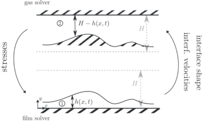
aretheratioofviscositiesanddensities,respectively.Forwhatconcernsthegas,thetop wallisrigidandfixed,inawaythattheboundaryconditionsyield

Fig. 3. Sketch of film (bottom) and gas (top) solver geometries. In the background, dashed lines indicate the base configuration, i.e.Fig. 1. The liquid filmtransfers to the gasthe velocity andthe position ofthe interface:Navier–Stokes equations(27) arethus solvedbymeansofthecontinuityofvelocitiesandthekinematiccondition,namely

u2

|

h

=

u1

|

h

,

v2

|

h

=

v1

|

h

.

(32)

Thesystemisclosedbythederivationofu1

|

h throughtheleading-ordervelocityprofile(16),beingthefirst-ordervelocity

notnecessary(seeSection5.3.1).At y

₌

h,expression(16)leadsto

u1

|

h

=

3 2 q1 h

+

1 4

τ

ih

,

(33)

while v1

|

h isdirectlyobtainedbythekinematiccondition

∂

th

+

u

|

h

∂

xh

=

v

|

h.

5. Thenumericalapproach

Inthe computationalanalysis, wetreat thetwo-layerchannel flowofFig. 1 withperiodic boundaryconditionsonleft andrightsides,whiletopandbottomsidesarerigidwalls.Periodicboundaryconditionsassurethattheflowgoingoutof thedomainisreinjected attheentrance,verifyingtheconditionsofclosedflow.Meanwhile,duetotheperiodic boundary conditions, the wavelength, ratherthan the frequency, must be imposed in the performed computational investigations. Initialconditionscorrespondtotheperturbedequilibriumstate.

WedividethechannelgeometryofFig. 1intotwoframeworks,whichrepresentthestructuresoftwodistinctsolversto bepresentedinthefollowing:thebottomofFig. 3isreferredtothefilmsolver,whilethetopofFig. 3tothegassolver.The film solverallowsustostudyashearedliquidfilmflowingonaflat andrigidwall,andisbasedonthelow-dimensional film model (24)–(26) previously introduced. Thedomain of resolutionof such equationsis

Ä

1

= {

0

≤ ˜

x

≤ ˜

L

}

,where

˜

L is the length of the channel. On the contrary, the gas solver is used to describe a laminar gas bounded on the top by a rigid andfixed wall, andon the bottom by a liquid film, which is modeled asa wavy wall witha certain motion. The gas solverworkswithequations (27)andaccountsformoving meshes. Thedomain ofresolutionofthe gasequationsis

Ä

2

(˜

t

)

= {

0

_{≤ ˜}

x

_{≤ ˜}

L

_{; ˜}

h

(˜

x

,

t

˜

)

≤ ˜

y

_{≤ ˜}

H

_}

. Furthermore,ashighlighted inFig. 3, thetwo solvers exchange informationsat the interface. Particularly, following the previous section, we chooseto provide interfacial shear stress andpressure gradient from the gas solver to the film, while the film solver returns to the gas shape andvelocity of the interface. This data exchangepermitstomodeltheinterfaceandallmutualeffectsbetweentheliquidandthegas.

Thischoiceofcouplingmethodologyiscoherentwiththefactthatthelong-wavemodel(24)computesfilmthicknessh

andflowrateq,whicharedirectlytransferredtothegassolverwithoutfurthermanipulations,exceptforrecoveringthe in-terfacialvelocity(33).However,otherchoicesofliquid–gascouplingarepossible.Forexample,werefertoHabchietal.[38], whohavestudiedliquid–gasindustrialproblemsbyusinganorder-zerofilmmodelfortheliquidphase,thusneglectingthe correction atorderone ofthewall shearstress,aswell astheretro-actionofthe liquidgivenbythe deformationofthe interface;wealsorefertotheaforementionedworkofTseluiko &Kalliadasis[26] forcounter-currentturbulentflows over awavyliquidfilm.

Anotherinterestingfeatureofourcouplingmethodologyconcernsthesurfacetensiondiscretization.Indeed,giventhat thefilmsolvertransferstothegasthepositionoftheinterfacebymeansoftheALEmethod,thesurfacetensionhasnotto beimplementedintothegassolver.Thegascanseetheeffectsofthesurfacetensionbythedeformation oftheinterface, which iscomputedateach time step bythe filmsolver takingintoaccount thecapillaryeffects, inaccordancewiththe hydrostaticpressure(11).ThisallowstoavoidthediscretizationofthesurfacetensiontermintheNavier–Stokesanalysis. As a consequence,ifthecapillarycharacteristic timeis thesmallest, we can getgreater time stepsin thecomputational investigations,comparedtotheclassicalfullDNS.

However,itmustbestatedthatthegasfeelsthestressesoftheliquidbyanindirectwayonly,i.e.throughthetransferof theboundaryandtheinterfacial velocities.Aconsequenceofthismightbethatthestressesfromtheliquidareneglected:

theanswer to thisissuecan be addressedby testingthecoupling methodologyto the caseoftwo layers ofcomparable viscosities, which thiswork does not. We leave thus thismatter to future studies. Secondly,it is worthwhile to discuss abouttheconsequencesofthe long-wavemodel (24)onthecouplingtechnique. Indeed,thelong-wave modeldeveloped inSection 3isbasedontheassumptionthattheshearstress

_τ

i andthepressuregradient

−

G areboundedforcoherence

oftheasymptoticanalysis. Thisleads tolimit thefunctionalityofSWANSto caseswherethegas velocitydoesnot reach extremelyhighvalues,i.e.whenthefilmbecomesexcessivelythinandatomizes.

Thissectionisstructuredas:firstlyweshow thenumericalschemesofthefilmsolver(Section 5.1) andthegassolver (Section5.2),secondlywediscussthenumericalcouplingbetweenthem(Section5.3).

5.1. Discreteone-layerdepth-integratedequationsforthefilmsolver

Webuildthefilmsolver(bottomofFig. 3)bydiscretizationofthedepth-integratedequations(24).Sincethelong-wave modelisbased onintegratedvariables, inthenumericalapproach one singlecellinthe verticaldirectionis sufficientto computethefilm.

FollowingtheworkofNoble&Vila[39]formulatedfortheEuler–Kortewegsystem,wehavediscretizeddepth-integrated equations (24)through an augmented system. This method consistsin reducing the order of the systemby adding one evolutionequationforthesurface tension,asshownbelow.Thisneedarisesfromthediscretizationofthesurfacetension whichinvolvesthirdderivatives,i.e.

∂

3xh,andfortheconsequentstabilityofdifferenceapproximationschemes.

Therefore,we havetaken the approach of Noble & Vila [39] andextended it to the depth-integrated equations (24), describingliquidfilmsdriven byshearstress andpressuregradient.Ifoneintroducesthequantity w

₌

√

σ

∂

xh

/

√

h,where

σ

=

We−1 _{isthecapillarycoefficientoftheintegratedequations,system(24)takestheform}

∂

th

+ ∂

x

(

hU

)

=

0

,

(34)

∂

t

(

hU

)

+ ∂

x

(

hU2

+

P

)

=

1 Re

h

3

h

₋

3U h

+

3 2

τ

i

−

T

i

+ ∂

x

(

ϕ

(

h

)∂

xw

) ,

(35)

∂

t

(

hw

)

+ ∂

x

(

hU w

)

= −∂

x

(

ϕ

(

h

)∂

xU

) ,

(36)

whereU

₌

q

/

h and

ϕ

(

h

)

=

h3/2

√

_σ

_{.Equation(36)hasbeenobtainedaftermultiplicationofthecontinuityequationby}

√

_h

_σ

andsubsequentderivationwithrespect to x.Itis worthwhileto mentionthat developingtheterm

∂

x

(

ϕ

(

h

)∂

xw

)

intothe

equation(35),weexactlygetthesurfacetensiontermofsystem(24).Asamatteroffact,thankstotheevolutionequation forw,theresultingsystemthuscontainsonlysecondderivativesinx.

FollowingNoble&Vila[39],system(34)–(36)canbewrittenintheconservativeform

∂

tv

+ ∂

xf

(

v

)

=

s

(

v

)

+ ∂

x

(

B

(

h

)∂

xz

) ,

(37)

where v

_{= (}

h

,

hU

,

hw

)

T is theconserved variablevector of depth-integratedequationsand f

(

v

)

= (

hU

,

hU2

₊

P

,

hU w

)

T thecorrespondingflux.Vectors

(

v

),

matrixB

(

h

)

andtheproductB

(

h

)∂

xz aredefinedas

s

(

v

)

=











0 1 Re

h

3

h

₋

3U_h

₊

3₂

τ

i

−

T

i

0











,

B

(

h

)

=





0 0 0 0 0

ϕ

0

₋

ϕ

0



 ,

B

(

h

)∂

xz

=







0

ϕ

∂

xw

−

ϕ

∂

xU







,

(38)

where z

_{= ∇}

vE

(

v

)

= ((

U2

/2

+

w2

/2)

+

F′

,

U

,

w

)

ifwe define thetotal energyasthe sumofkinetic andthermodynamic

freeenergies,namely E

₌

h

(

U2

/2

₊

w2

/2)

₊

F

(

h

).

Notethat function F

(

h

)

doesnot enterintheequation(37)giventhat thefirstcolumnofB

(

h

)

containsallzeros.

5.1.1. Spatio-temporaldiscretizationschemes

Discreteequationsofthefilmsolverhavebeenobtainedbymeansofasecond-orderaccuratespacediscretization,and theRusanovfluxfortheapproximateRiemannsolver.Indeed,onlyafewnumericalschemesappliedtoequations(34)–(36)

are foundto be entropystable, in thesense that corresponding difference approximationsdissipate theenergy, we refer to[39]forfurtherdetails.TimediscretizationiscomputedthroughtheHeun’smethod,whichcanbeseenasanimproved Euler’smethodoratwo-step Runge–Kuttamethod.Ifwe define vn

i astheaveragevalue ofv at timen withinthe celli,

namely vn_i

₌

1

1

x x

_Z

i+1/2 xi−1/2 vn

(

x

)

dx

,

(39)

andsimilarlyforsn

i,theintegrationofequations(37)overthecelli andthetimeinterval

(

n

,

n

+

1)leadsto

vn_i+1/2

₌

vn_i

₋

1

t

1

x

(

f n i+1/2

−

fin−1/2

)

+ 1

tsni

+

1

t

1

x2

[

B n i+1/2

(

zni+1

−

zni

)

−

Bni−1/2

(

zni

−

zni−1

)

] ,

(40)

and vn_i+1

₌

v n i

+

v n+1/2 i 2

−

1

t

1

x f_in₊+₁1_//₂2

₋

f_in₋+₁1_//₂2 2

+

1

₂t

"

sn_i+1/2

₊

1

1

x2

³

Bn_i+1/2 +1/2

(

zn+ 1/2 i+1

−

zn+ 1/2 i

)

−

B n+1/2 i−1/2

(

zn+ 1/2 i

−

z n+1/2 i−1

)

´

#

,

(41)

where superscript n

₊

1/2 refers to quantities evaluated at the first step ofHeun’s method. Indices i, i

₊

1, i

₋

1 refer to central, right andleft cells respectively, while i

₊

1/2 and i

₋

1/2 specifyinterface values,where flux f and matrix

B,as well asderivatives

∂

xz,must be evaluated. Thediscrete quantity fin+1/2 is solved withthe Rusanovscheme, which is demonstrated tobe entropystablefortheEuler–Korteweg equation,see [39].Omitting thesuperscript n,Rusanovflux yields(Toro[40]) fi+1/2

=

f

(

v+_i+1/2

)

₊

f

(

v−_i+1/2

)

2

−

i+max1/2±

[

U

+

e

]

v+_i+1/2

₋

v−_i+1/2 2

,

(42)

where U

₌

vy

/

vx ande2

=

d P

/

dh isthecharacteristicvelocity, with P “pressure”termdefinedin(25).Quantities v+_i+1/2

andv−_i+1/2 aretherightandleft statesacrosstheinterface ini

₊

1/2,respectively,andhavebeenfoundthroughaMUSCL spacediscretization.Furthermore,

(

zn_i+1

₋

zn_i

)/1

x approximates

∂

xzn attheinterface i

+

1/2,wherezn_i represents z within

the cell i at time n. In order to write the matrix B at the interface, we use a central discretization, namely

_ϕ

i+1/2

=

√

_σ

((

hi+1

+

hi

)/2)

3/2 fromthedefinitionof

ϕ

givenin(36).

Recallingthemomentumequation(35)oftheaugmentedsystemofdepth-integratedequations,thesourcetermcontains spaceandtime derivativesofinterfacial shearstress

_τ

i andpressuregradient

−

G providedbythe gastothe liquidfilm,

throughthetermT definedin(26).Spacederivativeshavebeendiscretizedbymeansofcentraldifferenceapproximations, namely

(∂

x

τ

i

)

ni

=

(

τ

i

)

ni+1

− (

τ

i

)

ni−1 2

1

x

,

(∂

xG

)

n i

=

Gn_i+1

₋

Gn_i−1 2

1

x

,

(43)

whilerespectivetimederivativeshavebeenapproximatedwithabackwarddiscretization,thatis

(∂

t

τ

i

)

ni

=

(

τ

i

)

ni

− (

τ

i

)

n_i−1

1

t

,

(∂

tG

)

n i

=

Gn i

−

G n−1 i

1

t

.

(44)

5.1.2. Stabilityoftheschemeforthefilmsolver

The characteristic velocity e2

₌

₄₅2

3

2h4

₊

₁₅4

3

τ

ih3

+

1₄

τ

_i2h2

+

_Frh cos

β

must be positive in order to have hyperbolic

equations(Whitham[41]).Particularly,alltermsofe2 arealwayspositive,withtheexceptionof

3

τ

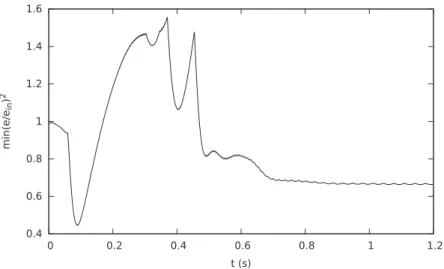
i:asaconsequence,the

signofe2 hastobealwaysverifieda posteriori.Forexample,Fig. 4showsthetimeevolutionofminimumnormalizede2

corresponding tothetesttobeanalyzedinSection6: anair–watersystemflowinginaconfinedchannelwithRe1

=

4.48 andRe2

=

36.8.Itisshownthatinthisconfiguratione2isalwayspositiveandtheequationsarethushyperbolic.

For what concerns the Courant–Friedrichs–Lewy (CFL) condition of the scheme, the non-linear stability provides

1

t

1

x−2

_<

_const

_.,

_{the constant value depending from the initial data, for first-order space discretizations (Corollary 3.4} of[39]).Nevertheless,weuseasecond-orderspacediscretization,forwhichanecessarylinearstabilityconditionis (Corol-lary 2.6of[39]forLax–Friedrichsscheme)

1

t

1

x

³

U

₊

r

e2

₊

2

σ

1

x2

´

≤

1

.

(45)

5.2. DiscretecompressibleNavier–Stokesequationsforthegassolver

The systemof Navier–Stokes equations (27) has been discretized witha first-order spatio-temporal discretization by usingalow-MachschemeinadditiontotheALEtechnique.Thelow-Machscheme,basedontheworkofGrenieretal.[42], allows solving compressibleflows atlowspeeds, where classicalapproximateRiemann solvers arevery dissipative,given thattheflowvelocityismuchsmallerthanthesoundcelerity.

TheALEtechniqueisinsteadusedtocouplethelow-Machschemewiththediscretedepth-integratedequations(34)–(36)

fortheliquidphase,andwillbedetailedlater.

Before the analysis of the discrete equations and the low-Mach scheme, we show how the Navier–Stokes equations are modified by the node motion of the grid. Recallingthe equations (27), thissystem can be written as(omitting the subscript 2)

Fig. 4. Timeevolutionoftheminimumcharacteristicvelocitye2normalizedwiththeinitialvalueein=2.5·10−4m2s−2.Two-layerflowwithdimensionless numbers:Re1=4.48,Re2=36.8,Fr=0.93,We=0.002,andgeometrygivenbyH˜=0.39 mm andλ=26 mm.After0.7 speriodicwavesappear.

whereLu

= ∂

t

φ

+ ∇ · (φ ⊗

u

),

andF

=

ρ

Fr−1

(

gx

,

gy

)

T.The vector

φ

= (

ρ

,

ρ

u

,

ρ

v

)

T istheconservedvariablevector,while

6

E isthe“pressurecontribution”ofthestresstensor

6

= −6

E

₊

_{T.Thesearedefinedas}

6

Ex

=







0

5

0







,

6

E y

=







0 0

5







,

Tx

=







0 Txx Txy







,

Ty

=







0 Txy Ty y







,

(47)

where

5

=

γ

₂−1M−2p.Whenthegridmoves,ameshvelocityhastobeinvolvedintotheNavier–Stokesequations,andwe introducea generic meshvelocity u for

_ˆ

each edge,to be definedlater,corresponding to thenode motion.Therefore,the

effectofthearbitrarymotionofthecomputationalmeshleadstorewriteequations(46)as

L_uˆ

= −∇ · [6

E

+ φ ⊗ (

u

− ˆ

u

)

] +

Re−1

∇ ·

T

+

F

,

(48)

whereLu_ˆ

= ∂

t

φ

+ ∇ · (φ ⊗ ˆ

u

).

Finally,themotionofthegridmodifiesonlytheinviscidsideoftheequations.

5.2.1. Low-Machschemedescription

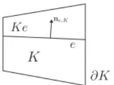
Inordertodeveloptheabovementionedlow-Machschemeanddiscretizeequations(48),Fig. 5showsthenotationused inthefollowing forthedevelopment ofdiscreteequations: K designates thecell,Ke itsneighborhood cells andne,K the

outwardnormalcorrespondingtotheedge e.Therefore,followingGrenieretal.[42],equations(48)arediscretizedas

ρ

n_K+1

=

m n K mn_K+1

ρ

n K

−

1

t mn_K+1

X

e∈∂K

³

l−

ρ

_Ken+1

+

l+

ρ

_Kn+1

´

mn_e+1

,

(49)

ρ

n_K+1un_K+1

₌

m n K mn_K+1

ρ

n KunK

+

1

t mn_K+1

X

e∈∂K

³

l−

ρ

_Ken+1u_Ken

₊

l+

ρ

n_K+1un_K

_{+ 5}

n_e+1nn_e+_,K1

´

mn_e+1

+ 1

t m n K mn_K+1F n+1 K

+

Re−1 mn_K+1

X

e∈∂K Tn_e

_·

nn_e,+_K1mn_e+1

,

(50)

where

∂

K isthecellcontour,mK thecellsurfaceandmethelengthofeachedge.Superscriptsn andn

+

1 refertothetime

step.Wealsodefine

l−

₌

min

_[

wn_e

_·

nn_e,+_K1

,

0

_{] − Ŵ}

emax

[5

n_Ke+1

− 5

n_K+1

,

0

] ,

(51a)

l+

₌

max

_[

wn_e

_·

nn_e+_,K1

,

0

] − Ŵ

emin

[5

nKe+1

− 5

n+1 K

,

0

] ,

(51b) wn_e

=

1₂

(

un_K

+

un_Ke

)

− ˆ

un_e

,

(51c)

5

ne+1

=

1 2

(5

n+1 K

+ 5

n+1 Ke

) .

(51d)

Parameter

Ŵ

e isinsteadapositivecoefficienttobeadjustedforthestabilityofthescheme(seeSection 5.2.2).Thevelocity wn_e defined on the edge e at time n takes into account also the ALE velocity u

ˆ

n_e, to be defined later. Furthermore, the pressurep canbewrittenasafunctionofthedensity

ρ

bylinearizingtheequationofstatearoundthebasestate.

Fig. 5. Notations for the low-Mach scheme used in this work.

Some remarksmustbedone abouttheequations (49)–(51).Asalreadystated,thoseare basedontheworkofGrenier et al.[42] fortwo-phase flows. However, we highlightthe main differences:firstly, inthiswork the equations(49)–(51)

are usedfor asinglephase, thatis thegas.In addition,we haveextended thework ofGrenier etal.[42] by addingthe possibilityofmovingmeshes.Wecannoticethatthemovingmeshmanifestsitselfbythepresenceoftheedgevelocityu

ˆ

n e

in(51c).Asaconsequence,boththeedgelengthandcellsurfacearedifferentfromthoseattheprevioustimestep,which makesthedifferencebetweenmn

e andmnK withmne+1 andmnK+1,respectively.WealsorecallthatintheALEframeworkwe

have d

dt

(

m

(

t

))

= ∇ ·

¡

ˆ

u

¢

.

Forwhatconcernstheviscousstress tensor,giventhedefinition(28),itsdiscretizationturnsintothereconstructionof thevelocitygradientoneveryedgestartingfromtheaveragevelocityinthecenterofeachcell.Wewillnotdetailherethe methodusedfornon-orthogonalmeshes,whichisbasedonthediamondcellstrategy,andrefertoCoudièreetal.[43].

5.2.2. Energystabilityofthegassolver

Thestability ofthelow-Mach schemeisanalyzedasinGrenier etal.[42],andwegetthatthetotalfreeenergyofthe flowisatimedecreasingfunction.WedefinethetotalfreeenergyofthesystemasE

₌

1₂

ρ

k

u

k

2

+ 8

,with

8

=

ρ

R

_̺̺

∗

p(r) r2 dr

corresponding to the barotropic pressure.Following the samecalculations asinthe stability proof of[42],we write the discreteenergyequationas(omittingviscoustermsandgravity)

mn_K+1En_K+1

₋

mn_KEn_K

_{+ 1}

t

X

e∈∂K

h

(

wn_e

_·

nn_e,+_K1

)

+En_K+1

_{+ (}

wn_e

_·

nn_e,+_K1

)

−

ρ

_Ken+1En_Ke+1

i

mn_e+1

+

1

₂t

X

e∈∂K

h³

un_K

5

n_Ke+1

+ 5

nK+1unKe

´

·

nn_e,+_K1mn_e+1

_{− Ŵ}

e

³

5

n_Ke+1

+ 5

nK+1

´ ³

5

n_Ke+1

− 5

nK+1

´

mn_e+1

i

=

mn_K+1

¡

Qn_K

₊

Rn_K

¢

_{+ 1}

t Sn_K

.

(52)

Here,superscripts

₊

,

₋

denotemax

_[·,

0

_]

,min

_[·,

0

_]

respectively.Defining

8

′

=

κ

,byaTaylorexpansionof

8

thereexists a certain

θ

∈ [

0,1

_]

suchthat

8(

ρ

n_K+1

)

− 8(

ρ

n_K

)

= (

ρ

n_K

−

ρ

n_K

)

κ

_Kn+1

−

1₂

e

κ

′_Kn+1

(

ρ

n_K

−

ρ

n_K

)

2

,

where

e

κ

′Kn+1

=

κ

′

((1

− θ)

ρ

nK

+ θ

ρ

n+1

K

),

andsimilarlyfor

e

κ

e′n+1.Notealsothat

κ

′

=

a2

ρ

−1

>

0.

mn_K+1Qn_K

₌

mn_K+11 2

ρ

n+1 K

°

°

°

un_K+1

₋

un_K

°

°

°

2

+ 1

t

X

e∈∂K

(

wn_e

_·

n_en_,+_K1

)

−

ρ

_Ken+11 2

°

°

un_Ke

₋

un_K

°

°

2mn_e+1

−

1

₂t

X

e∈∂K

Ŵ

e

³

5

n_Ke+1

− 5

nK+1

´2

mn_e+1

,

(53a) mn_K+1Rn_K

_{= −}

1 2m n K

e

κ

K′n+1

³

ρ

n_K+1

−

ρ

nK

´2

+

1₂

1

t

X

e∈∂K

(

wn_e

_·

n_en_,+_K1

)

−

e

κ

e′n+1

³

ρ

_Kn+1

−

ρ

_Ken+1

´2

mn_e+1

,

(53b) Sn_K

_{= −5}

n_K+1

ÃÃ

mn_K+1

₋

mn K

1

t

!

−

X

e∈∂K

(

u

ˆ

n_e

_·

nn_e+_,K1

)

mn_e+1

!

.

(53c)

UsingtheCauchy–Schwarzinequality,thetermQn_K canbeestimatedas

Q_Kn

_≤

1

t 2mn+1 K

Ã

X

e∈∂K

Ã

1

t 2mn+1 K

ρ

n+1 K mn_∂+_K1

_{− Ŵ}

e

!

_³

5

n_Ke+1

− 5

nK+1

´2

mn_e+1

!

+

Ã

1

₋

2

1

t mn_K+1

ρ

n_K+1

³ X

e∈∂K

(

−

wn_e

·

nn_e+_,K1

)

−

ρ

n_Ke+1mn_e+1

´

! Ã

1

t mn_K+1

X

e∈∂K

(

wn_e

·

n_en_,+_K1

)

−

ρ

_Ken+11 2

°

°

un_Ke

−

un_K

°

°

2mn_e+1

!

.

We notice that Rn_K in (53b) is negative because

(

wn_e

_·

nn_e,+_K1

)

−

≤

0, while Qn_K is negative ifthe following conditions are satisfied:

Fig. 6. Sketch of the coupling methodology and time progress n−→n+1.

1

t

_≤

1

m 2lK

,

Ŵ

e

≥ 1

t max

"

mn_∂+_K1 2

ρ

n_K+1mn_K+1

,

mn_∂+_{K e}1 2

ρ

_Ken+1mn_Ke+1

#

,

(54)

wherelK and

1

m aredefinedas

lK

=

1

ρ

n_K+1mn_∂+_K1

X

e∈∂K

|

l−

_|

ρ

_Ken+1mn_e+1

,

1

m

₌

m n+1 K mn_∂+_K1

,

(55)

wherel−_{isin(51a).Onenoticesthat thediscretemassconservationequation(49)isimplicit, permittingtorelaxtheCFL}

condition(54)ofthescheme,becausethestabilityconditiondoesnotcontainthesoundcelerity.Concerningtheterm Sn_K

in(53c),itcanbeconsideredzeroiffulfillsexactlythecorrespondingdiscretegeometricconservation(DCGL),seeFarhatet al.[44].Indeed,wenoticethat(53c)isadiscreteversion of d

dt

(

m

(

t

))

= ∇ ·

¡

ˆ

u

¢

whichisthebasicruleformeshevolution

intheALEframework.Inthiscasewehavethusproventhat

X

K

mn_K+1En_K+1

_≤

X

K

mn_KEn_K

.

(56)

Ifweonlyhavefirstorderconsistencyofthegeometricconservation,ratherthanexactdiscretegeometricconservation,we getthat d

dt

(

m

(

t

))

− ∇ ·

¡

ˆ

u

¢

_{= O(}

mn_K+1

1

t

),

andwekeepacontrolofthetotalenergyineCt _{throughGronwall’slemma.We}

refer toDonea etal.[45] for additionalreferences aboutDCGLand toLanson &Vila [46] forstability proof ofALE type schemesforconservationlaws.

5.3.Couplingapproachdevelopment

Afterthedescriptionoffilmandgassolvers,wediscussthenumericalcouplingbetweenthetwo.Fig. 6summarizesall stepsofthecouplingprocessintherange

(

n

,

n

₊

1):

1. thefilmsolvercomputesfilmthicknessh andaveragevelocityU attimeleveln

₊

1.Bydoingso,equation(35)shows thatinterfacial shearstress

_τ

i andpressuregradient

−

G,aswell astheir respectivespatio-temporal derivativesmust

beknown.Thesearegiveneitherfromthepreviouscomputationattimen orfromtheinitialconditionsattimet

₌

0; 2. filmthicknesshn+1 _{andaveragevelocityU}n+1 _{canbethenusedtoevaluatethevelocityfield attheinterface,namely}

(

u

_|

h

)

n+1 and

(

v

|

h

)

n+1 (asshowninSection4),andthedisplacementoftheinterfacewithrespecttotheprevioustime

step;

3. subsequently, theposition of the interface at time n

₊

1 can be manipulated to update the mesh ofthe gas solver. The bottom cell of the grid movesexactly as the interface, while the motion of all other nodes is submitted to a mesh-updatelaw,tobediscussedlater;

5. the gassolver takesasinput theinterfacial velocities, theupdated mesh andthevelocity u to

_ˆ

compute densityand velocityfieldsattimestepn

₊

1 (low-Machschemepreviouslydiscussed);

6. finally, interfacialshearstress

_τ

n+1

i andpressuregradient

−

Gn+1 canbecomputed, aswellastheirrespective

spatio-temporalderivativesbymeansofcentraldifferenceandbackwarddiscretization(see(43)and(44)).

This couplingmethodologyapplies afirst-ordertime discretizationandis explicit,in awaythat thegassolver adoptsat time leveln the outputprovided bythefilm evaluatedatthe stepn

₊

1.As aconsequence,thetime stepis imposedby theminimumbetweenthetwosolvers.Incertain configurations,theviscoustime steptv

≃ 1

y2

/

ν

g representsthelower

limit,sincewetreatthediscreteviscoustermexplicitly.Otherwise,thetimestepisimposedbythefilmstabilitycondition (see(45)),inparticularwhenwerefineinthex-direction.

Themaineffectofthetime-explicitcouplingtechniqueisthatthetime-scaleratiointhegasandintheliquidmustbe high.Inotherwords,thefilmcannotcapturethephenomenafasterthanitstimescalingh

˜

0

/ ˜

U0.Forexample,thiswouldbe thecaseoftheacousticeffectsinthegas,althoughintheperformedteststhosearenegligible,asshownlater(Section6.1.3).

5.3.1. Filmtogascoupling

Asalreadystated,thefilmsolvertakesinterfacialshearstress

_τ

iandpressuregradient

−

G asinputforthecomputation

of film thickness h and average velocity U , following the numerical scheme (37). Nevertheless, the gas solver requires velocitiesevaluatedattheinterface,aswellasthedisplacementoftheinterfaceateachtimestep.

From the average velocity U , one can obtain the interfacial longitudinal velocity u

_|

h by means of the asymptotic

ex-pansion discussed in Section 3.1. Particularly, the leading-order velocity profile (16) is used to evaluate the interfacial longitudinalvelocityu

_|

h at

O(1),

namely

(

u

_|

h

)

n_i+1

=

3 2U n+1 i

+

1 4

(

τ

i

)

n i

,

(57)

where the use of the shear stress at time n is due to the explicit coupling methodology which causes a delay of the evaluationprocess.Theeffectoftransferringtheleading-orderinterfacialvelocityfromthefilmtothegasisagoodestimate, giventhat theinterface iscomputedat

O(

ε

).

Indeed,first-ordervelocitiesgreatlymodify theinterfaceshape, butremain verysmallcomparedtoleading-order’s.Forwhatconcernsthetransversalinterfacialvelocity,thekinematiccondition(10c)

yields

(

v

_|

h

)

n_i+1

= (∂

th

)

n_i+1

+ (

u

|

h

)

n_i+1

(∂

xh

)

n_i+1

,

(58)

afterappropriatediscretizationof

∂

x,th withcentraldifferenceandbackwardapproximations,namely

(∂

xh

)

n_i+1

=

hn_i++₁1

₋

hn_i−+₁1 2

1

x

,

(∂

th

)

n+1 i

=

hn_i+1

₋

hn_i

1

t

.

(59)

5.3.2. ALEmethoddevelopment

In this section, we discuss the development of the ALE technique. This technique is a combination of Eulerian and Lagrangianapproaches,sincethenodesofthegridcanmovearbitrarily.

In the low-Mach computational schemepreviously described, we choose that grid nodescan move along thevertical direction only. Therefore, the initial rectangular shape of the cells of the gas turn possibly into trapezoid, because left and rightedges remain always parallel toeach other,assketched in Figs. 7–8.Instead, we recall that the film solver is one-dimensionalbecauseoftheintegralformulation. Giventhepositionoftheinterfaceatthetimestepn

₊

1 andinthe centerofeachfilmcell,sayhn_i+1,onecanrecoverthepositionofeachcorrespondingnoderelativetotheequilibriumstate

h0 (equalforeverycell),namely

δ

_in₊+₁1_/2

=

h

n+1

i+1

+

hni+1

2

−

h0

.

(60)

Subsequently,throughtherelationdhn_i++₁1_/2

_{= δ}

_in₊+₁1_/2

_{− δ}

n

i+1/2,therelativemotionoftheinterfaceduringtime issent tothe gas toupdate each bottom node ofthe grid.Note that dh_in₊+₁1_/2 is thedisplacement ofthe gasmesh forall nodesinthe bottom, attime n

₊

1, assketchedinFig. 7.However, we requirea mesh-updatemethodology whichgeneratesthe new meshateachtimestep.Sincewewanttokeepthegridasregularaspossiblewiththeaimtoavoidstrongmeshdistortions, asimplealgebraiclawisusedtotransfertheinterfacedisplacementdhn_i++₁1_/2toallothernodesintheverticaldirection,but otherchoicesarepossible.

AnotherrelevantfeatureoftheALEtechniqueisthevelocity assignedtoeachnode.Inthiswork,sincethegridmoves only in the y-direction, the longitudinal component u of

_ˆ

the ALE velocity vanishes, namely u

ˆ

_{= (}

0,v

_ˆ

)

T. The y-velocity componentv is

ˆ

definedforeveryedge,basedonthedisplacementofthenodesatbothsidesoftheedge.Itreads

ˆ

ve

=

1

dt

(

dhN1

+

dhN2

) ,

(61)