Science Arts & Métiers (SAM)
is an open access repository that collects the work of Arts et Métiers Institute of
Technology researchers and makes it freely available over the web where possible.
This is an author-deposited version published in: https://sam.ensam.eu
Handle ID: .http://hdl.handle.net/10985/8759
To cite this version :
Jean-Marie LE YAOUANC, Eric SAUX, Christophe CLARAMUNT - A Visibility and Spatial Constraint-Based Approach for Geopositioning - In: 6th international conference on Geographic Information Science (GIScience 2010), Switzerland, 201009 Geographic Information Science -2010
Any correspondence concerning this service should be sent to the repository Administrator : [email protected]
A Visibility and Spatial Constraint-based
Approach for Geopositioning
Jean-Marie Le Yaouanc, Éric Saux, Christophe Claramunt
Naval Academy Research Institute, CC 600, Lanvéoc, 29240 Brest Cedex 9, France {leyaouanc, saux, claramunt}@ecole-navale.fr
Abstract. Over the past decade, automated systems dedicated to geopositioning have been the object of considerable development. De-spite the success of these systems for many applications, they cannot be directly applied to qualitative descriptions of space. The research pre-sented in this paper introduces a visibility and constraint-based approach whose objective is to locate an observer from the verbal description of his/her surroundings. The geopositioning process is formally supported by a constraint-satisfaction algorithm. Preliminary experiments are ap-plied to the description of environmental scenes.
Key words: Landscape perception, place descriptions, scene-finding ap-proach, geopositioning.
1
Introduction
Geopositioning is a process whose objective is to relate a geographic location to a given entity, activity or person. This is supported by qualitative references to locations we employ in everyday discourse, e.g. place-names, and quantitative representations used in many activities based on coordinates-based navigation. Early geopositioning systems have been widely applied to quantitative models and geometrical representations of space. Despite the interest of these approaches for cartographical applications, they do not completely reflect the way a human perceives and describes his/her environment since he/she preferably stores and processes qualitative information. This is particularly relevant for natural en-vironments since they do not have well-defined emerging structures similar to those present in an urban environment. Perception encompasses cognitive prin-ciples that favor memorization of the main properties of an environment, and potentially communication of these properties to an external addressee using natural language [1,2]. These descriptions are essentially qualitative and based on common sense, i.e., intuitive concepts we daily manipulate to interact with our environment [3,4,5].
While the interpretation of spatial relations for the location of entities has long been studied, they have been hardly considered for the geopositioning of an observer perceiving his environment. The objective of the research presented in
this paper consists in developing a model suitable with perception and spatial cognition, but also appropriated for the processing of quantitative spatial data. We consider the case of an observer located at a fixed vantage in a natural
landscape, perceiving his/her 360◦ surroundings, and who is asked to provide
a description of his environment to an external addressee. The description of such an environment underlines the salient entities of space, the spatial relations between them, and the structural properties of the environment. Entities are identified according to a semantic categorization, their proximity and orientation with respect to the observer [6]. The research presented in this paper extends this modeling approach by identifying the possible locations of the observer from the interpretation of the description of his surroundings. It is supported by a visibility and constraint-based approach. This provides a support for search and rescue approaches by bridging the gap between a qualitative map resulting from the direct perception of a scene, and a quantitative representation of the environment given by a GIS database.
The remainder of the paper is organized as follows. Section 2 presents the modeling background of the approach and a conceptual representation of an en-vironmental scene. Section 3 introduces the context of this research and develops the modeling approach, based on the concept of visibility of salient entities and the interpretation of spatial relations as spatial constraints. Lastly, Section 4 draws the conclusions and outlines further work.
2
Modeling background
In a previous work, we have introduced a structural model of a scene generated from the interpretation of a verbal description. It identifies the salient entities, spatial relations between them, and spatial constructs of the landscape [6]. The spatial description is schematized by a representation that constitutes a
model-ing support for the study of environmental scenes, i.e., 360◦scenes perceived by
an observer from a fixed vantage viewpoint. The perception of an environment is closely associated to a cognitive organization that reflects different levels of perception [7]. Since humans tend to structure space using distance and bod-ily directions, an environmental scene is structured by four proximity spaces determined by their distance from the observer, and a directional cone-based partition [8] whose number can vary from two (front/back or right/left) to four (front, back, right and left).
Let us consider an example of scene description given by an observer to a distant addressee who is asked to consider the described environment: “ I am on a footpath that runs along a castle and a pond. In front of me, there is a little valley with the castle on the right of it and at the horizon, I can distinguish a mountain range. On my right is the farm of the castle. Behind me, there is the pond with a meadow behind, and a forest far away ”. In order to promote communication and cooperation, the observer contribution should be informative enough [9]. We assume that the resulting scene description can result from a preliminary complex dialogue between the observer and the addressee
for the settlement of inconsistencies and vagueness problems. In order to keep the relevant information, the description is first parsed and semi-automatically filtered by the Tinky parser [10]. Co-references are identified and resolved, and
the description is modeled as a set of triplets ui such as ui = [ej, rk, el] with
ej, el ∈ E the set of entities of an environmental scene, and rk ∈ R the set of
spatial relations. Distance and directional relations are interpreted with the use of an application ontology, and the identified entities are associated to one-to-many proximity spaces and directional cones. No matter the nature, prominence or familiarity of the considered objects, the spatial relations are interpreted in order to favor their relative ordering.
The resulting conceptual map of Figure 1 illustrates the spatial structure, diversity and relative ordering of the entities. Such a model qualifies and char-acterizes natural landscapes, and provides a framework for the analysis of the properties of the verbal descriptions made by different observers, and cross-comparisons of different landscape descriptions. However, the salient entities of the scene are not always clearly revealed. This has motivated the integration of salience scores, supported by a mutual reinforcement algorithm. It reflects the particularities of the entities that emerge from a scene description such as their linguistic properties, i.e., the richness of information associated to each term, and their structural characteristics, i.e., the degree of spatial isolation [11].
3
Geopositioning approach
Recent years have witnessed significant geopositioning developments, particu-larly when locations are not available using global positioning systems. This has been applied to search-and-rescue operations where the location of a hu-man (usually lost) should be retrieved. The ability of lost persons to precisely describe their perceived environment is essential to a successful identification of their location. The way people and particularly children behave and model their environment has been studied by cognitive studies, while cognitive distortions and reasons for retrieval failures have been qualified [12]. Preliminary experi-ments have explored the potential of GIS for the management of search teams [13], or the behavior of a lost person regarding her initial displacement plans, goals and own abilities [14]. However, GIS have not been used to the best of our knowledge for geopositioning an observer from a qualitative description and interpretation of his environment.
The description of the surroundings of the lost person is used as the only input of our approach. No assertion is made on their background, will, route, the reason why they planned the excursion, etc. The methodology used for the search of the observer results from the analysis of the verbal description. This is based on the interpretation of the entities and landmarks identified in the description, the spatial structure emerging from the proximity spaces that illustrate a relative ordering between the entities, and direction relations between the entities.
castle
Sentence n°1 Sentence n°2 Sentence n°3 Sentence n°4
FRONT BACK LEFT RIGHT meadow behind forest far away pond behind runs along footpath on valley in front of on the right of runs along mountain range at the horizon farm on the right of
Fig. 1. Conceptual map of a scene [6]
The geopositioning approach searches for the possible locations of the ob-server, and is applied as follows:
1. For each entity identified by the observer, computation of the viewsheds i.e., places for which each quoted entity can be perceived by the observer. 2. Interpretation of the direction relations derived from the directional cones
and identification of a new set of candidate solutions for the observer loca-tion.
3. Interpretation of the distance relations derived from the proximity spaces and identification of a new set of candidate solutions for the observer location.
4. Interpretation of the direction relations given relatively to entities, and iden-tification of a new set of candidate solutions for the observer location.
3.1 Visibility-based approach
Viewshed computation and analysis have long been applied in landscape and urban studies [15,16,17]. The main principle of a viewshed analysis is commonly determined by defining one location as the viewing point, and then calculating the line-of-sight to every other point within the region of interest. When the surface rises above the line of sight the target is out of sight, otherwise it is considered as in-sight [18,19]. The range of application is relatively large, from architectural studies where visibility represents a qualitative parameter for a site selection to minimize or maximize [20], to the distribution of forest-fire observation towers in natural environments [21].
The modeling approach should identify the possible locations of the entities quoted in the description. Let us assume that the described entities are directly visible from the fixed viewpoint of the observer. The visibility-based approach mainly focusses on the area from which the location of the entities can be viewed, as opposed to the visible area that is not equivalent because the height of the object at the viewing point may be different from the height of the viewed object [16]. Our objective is not to precisely locate the observer but rather the area the observer is supposed to be located at. Without loss of generality, we consider as equivalent the regions seen from a given entity and the ones visible from the observer.
Let us introduce the formal representation of the visibility-based approach.
Let E be the set of entities eiidentified in a verbal description D, S denotes the
ordered set of salient entities ei ∈ E, i.e., S = [e1, e2, . . . , en] and n denotes the
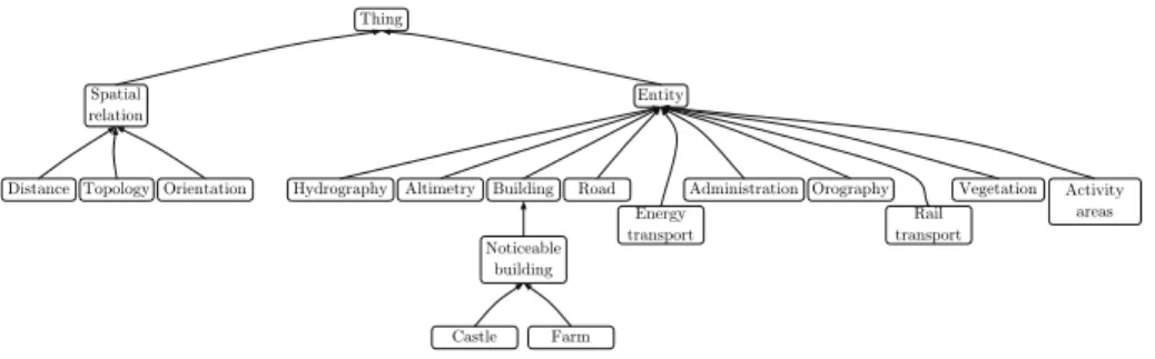
cardinality of set S. Let B be the set of objects of a GIS database considered as the repository of the region of interest. These objects and the relations material-ized in this GIS database are organmaterial-ized into a lattice of classes and sub-classes, that result from a classification provided by the French Institut Géographique National (Fig. 2).
Thing
Spatial
relation Entity
Distance Topology Orientation Hydrography Altimetry Building Road Energy transport Administration Orography Rail transport Vegetation Activity areas Noticeable building Castle Farm
Let C be the set of classes of the GIS database. The function fclass that
associates the class c ∈ C to an object bj∈ B is given by
fclass: B → C
bj 7→ c.
(1)
Similarly, the function gclass that associates the class c ∈ C to an entity
ei∈ S is given by
gclass: S → C
ei7→ c.
(2)
Let ei∈ S a salient entity of the verbal description. Since entity ei is visible
by the observer, the visibility-based approach should select all objects bj of the
database that correspond to the class of objects identified in the description as all could potentially be perceived by the observer. Let R denote the set of m objects bj ∈ B whose class fits that of entity ei, i.e., gclass(bj) = fclass(ei), and
i ∈ [0, . . . , m], j ∈ [0, . . . , n].
Let v be the function dedicated to the visibility computation. Let t be a digital terrain model, i.e. a triangulated irregular network that describes the
topography of the region of interest. Given an object bj located on terrain t, the
viewshed of bjis the set of points p of t from which bjis visible. We consider that
two points are defined as being visible to each other if a straight line can be drawn between the points without intersecting any part of the terrain surface between them, i.e., v(bj, t) = { p ∈ t / [bj, p] ∩ t = ∅ }. Let hvis(ei) be the function that
corresponds to the set of areas from which objects bj, j ∈ [1, . . . , m] of a similar
class than entity ei are visible. Then, hvis(ei) = {v(b1, t), . . . , v(bm, t)}.
Let Svis be a function that computes the possible locations of the
ob-server that result from the visibility-based approach. Svis is defined by the
intersection of the different viewsheds associated to each salient entity, i.e.,
Svis = T{hvis(ei)}, where i ∈ [1, . . . , n]. It is worth noting that the
salience-based approach enables to consider only the most salient entities rather than considering all of them. Afterwards, we shall however take into account all enti-ties.
Let us consider the example of description “ I am on a footpath that runs along a castle and a pond. In front of me, there is a little valley with the castle on the right of it ” and the resulting ordered set of salient entities S={“castle”,
“footpath”, “pond”, “valley”}. Firstly, the m objects bj of the database whose
class is “castle” are selected and each viewshed v(bj, t) is computed. If
ob-ject “castle” is the one considered, a solution for the possible location region
of the observer is given by the set of viewsheds of bj’s, i.e. hvis(castle) =
{v(b1, t), . . . , v(bm, t)}. The same method is applied to objects “footpath”, “pond”
and “valley”, and the visibility-based solution is provided by the intersection of
the viewsheds associated to each salient entity, i.e., Svis = {hvis(“castle00) ∩
hvis(“f ootpath00) ∩ hvis(“pond00) ∩ hvis(“valley00)}. The candidate objects are
those that can be perceived directly from the area given by the visibility-based solution, i.e., {bj, cj, dj, ej such as bj ∈ “castle00, cj ∈ “f ootpath00, dj ∈
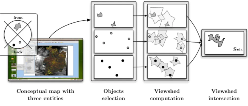
The visibility-based approach identifies the possible location areas where the observer can be located. Figure 3 summarizes the principle of this approach. This first step also identifies a set of physical objects of the environment that
could potentially be observed from the location regions Svis. This preliminary
filtering of the solution area will be refined in the following sub-sections by the interpretation of spatial relations between these objects and illustrated by the proximity spaces and directional cones.
Conceptual map with three entities front
back
Objects
selection computationViewshed intersectionViewshed Svis
Fig. 3. Visibility principle
3.2 Spatial relations as spatial constraints
Spatial relations are interpreted as spatial constraints that refine the possible locations of the observer. These spatial constraints are derived from the inter-pretation of linguistic expressions, and supported by the use of directional cones and proximity spaces of the conceptual map. This can be considered as a specific application of declarative modeling that is commonly applied to the automatic generation of an environment that corresponds to some linguistic descriptions. In particular, text-to-scene modeling has been used in many applications such as architectural design [22], and for the generation of virtual urban landscapes and animated scenes from road accident reports [23]. These modeling approaches are based on the interpretation of spatial constraints and semantic knowledge [24]. This is equivalent to a constraint satisfaction problem applied to the linguistic relations identified in an environment description [25]. A constraint-solver algo-rithm analyses the coherence or incoherence of the linguistic description in order to derive a possible representation of the scene.
The interpretation of the spatial relations quoted in the description is sup-ported by the directional cones and proximity spaces that structure the concep-tual map (Fig. 1). The principle consists in finding the limits of the location of the observer for which:
– The entity locations in the directional cones fulfill the linguistic description properties (Cases 1 and 2).
– Distance relations given relatively to the observer are geometrically inter-preted and supported by the use of proximity spaces (Case 3).
– Relative direction relations between two entities are geometrically inter-preted (Case 4).
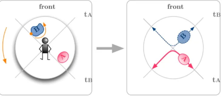
Case 1. Entities in opposite directional cones Let us consider two entities located into two opposite directional cones (front/back or right/left), i.e., enti-ties related to the observer by two opposite direction relations. The algorithm identifies the possible locations of the observer by computing the limits where object B is in front of the observer and object A is behind him, with a space
segmented by two straight lines tAand tBthat define the four directional cones,
i.e. front, back and right, left. Objects A and B of the database are fixed, and the principle illustrated by Figure 4 consists in identifying the limits of the solution that satisfies the directional constraints by moving the directional cones along the whole boundary of object B. This generates a relative displacement of object A while retaining its location in the back cone, and object B in the front cone. In order to get an exhaustive solution without losing possible locations due to approximation errors, we consider that an object that intersects the boundary
of a directional cone is in that directional cone. In such a case, tA (resp. tB) is
tangent to object A (resp. B).
B A A B front tA tB front tA tB
Fig. 4. Orientation constraint principle
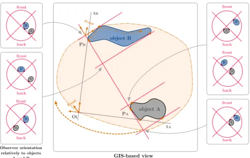
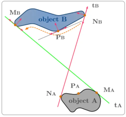
Let us consider two surface objects A and B (Fig.5), and PB (resp. PA)
the tangent point to B and tangent line tB (resp. tA). In order to identify the
observer location for which object B is in front of him, and object A behind,
space is discretized by uniformly moving point PB(resp. PA) along the boundary
of object B (resp. A). For each location of point PB (resp. PA),
1. Construction of tangent tB (resp. tA).
2. Construction of the exterior tangent tA to object A (resp. tB to object B)
that is also perpendicular to tB (resp. tA)1.
1
The interior tangent is not necessary since the resulting points are included in the solution.
object A object B tB PB PA B front back A Oi Front tA B front back A B front back A B front back A B front back A B front back A GIS-based view Observer orientation relatively to objects A and B Front
Fig. 5. Orientation constraint
The intersection Oiof tAwith tBgives a boundary point of the solution, i.e.,
a boundary point for the possible location of the observer. Consequently, the
region A(objectA, objectB) in which the observer should be located is bounded
by the convex hull materialized by points O1, . . . , Om with m ∈ N r {0}. The
algorithm is similar when objects A and/or B are modeled as polylines or points.
The difference with polylines is given by the intersection between tBand B (resp.
tAand A) that can then be a segment rather than a point.
Figure 5 illustrates the possible observer locations with respect to two objects A and B, when considering their relative locations to the observer. The solutions presented to the left and right of the figure show the range of the observer positions that fulfill the direction constraints. This algorithm is applied to all object pairs of the geographical database whose classes correspond to those of the entities located in two opposite directional cones. Let us consider the following example “ the castle is in front of me, and the valley behind ”, the previous algorithm is then applied to all object pairs (“castle”, “valley”) of the geographical
database that also belong to the previous solution Svis. Let EC1 be the set of
entities of the verbal description that are in a directional cone (e.g. Ef ront), and
EC2 the set of entities of the verbal description that are in the opposite cone
(e.g. Eback), EC1/2 the set of combinations of entity pairs (ei, ej) of the verbal
description with ei ∈ C1 and ej ∈ C2, OC1, OC2, OC1/2 the corresponding set
of objects and combinations of objects (om, on) of the GIS, and A(om, on) the
solution region with om∈ OC1 and on ∈ OC2. The solution region Sopposite_rel
for which some objects are in a cone (e.g. front) and others in the opposite one
directional cones, a possible solution Sdir is given by the intersection of the two
sub-solutions regions that correspond to the solutions front/back and right/left.
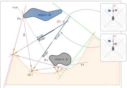
Let NB and MB denote the intersections of the interior tangents tA and
tB with object B. When space is partitioned by two subspaces, i.e., front/back
or right/left, the solution is given by uniformly moving point PB along the
boundary of object B from points NB to MB (Fig.6). For each PB, a solution
Si
PB given by the half space behind object B fulfills the constraint for which B
is in front of the observer (i.e., the observer is behind B). A similar method is
applied to object A. For each PA, a solution SPiAgiven by the half space is front
of object A. Sdir corresponds to the intersection of the two sub-constraints, i.e.,
Sdir= ∩(SPiB, S i PB). object A object B PB tA tB MB NB MA NA PA
Fig. 6. Orientation constraint (two cones)
Case 2. Entities in an identical cone Let us consider a second case where two entities are located in a same directional cone, i.e., entities related to the observer in a similar way. An equivalent algorithm is applied with the difference that it identifies the possible locations of the observer by computing the limits
for which objects A and B are in a same cone. The solution region Sdir_cone is
the complement of solution given by Case 1.
When space is partitioned by two directional cones (front/back or right/left),
the solution is constructed by uniformly moving point PB (resp. PA) along the
boundary of object B (resp. A) from points NB to MB (resp. NA to MA) that
constitutes the intersection of the exterior tangents tAand tB to object B (resp.
A). The solution is given by the exterior region bounded by the convex hull between A and B.
Case 3. Distance relations Distance relations, whether used in an egocentric or allocentric manner, are also integrated in the geopositioning process. Their
object A object B tAB PB PA Oi ProjA ProjB Proj A Proj B Mi B A Mi B A Mi t B tA
Fig. 7. Distance constraint
interpretation is given by the use of the proximity spaces that structure the con-ceptual map. When some entities are located in an identical directional cone, they can be located in different or similar proximity spaces with respect to the location of the observer. Figure 7 illustrates an example of distance constraint satisfaction where object A is in front of the observer, and B is behind A. The
space Sdistance that satisfies the two constraints also refers to the possible
loca-tions of the observer. The principle consists in finding the limits of the observer’s location with respect to the following constraints:
– Entities A and B are in an identical directional cone.
– Their distances relatively to the observer correspond to those supported by the conceptual map.
When searching for a candidate location of the observer relatively to objects A and B as illustrated in the previous example, the search method is as follows.
Space is uniformly discretized by uniformly moving point PB (resp. PA) along
the boundary of object B (resp. A). For each location of point PB (resp. PA),
tangents tBand tAare constructed. The relative ordering of the different entities
composing the environmental scene is defined by projecting entities A and B on
the median line that bisects angle \tA, tB (Fig. 7). The interval endpoints are
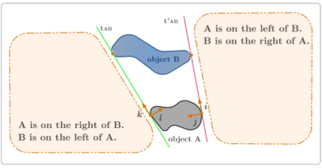
object A object B tAB t'AB A is on the left of B. B is on the right of A. A is on the right of B. B is on the left of A. i j k l
Fig. 8. Relative direction constraint
We consider that B is behind A when their endpoint beginnings (relatively to the observer) coincide. This search algorithm is similarly applied when the observed entities are represented as polylines. The difference is given by the fact that the
intersection between tB and B (resp. tA and A) can be a segment line rather
than just a point. However, it is worth noting that a partition of space based on two directional cones does not enable the identification of a candidate solution.
Case 4. Ternary direction relations Let us consider the case of a ternary relation using an observer-centered frame of reference [27], i.e., “on the left of ” or “on the right of ” between two distinct entities of an identical directional cone. If the observer identifies object A as being on the left of B, it means that he/she
is in a half-space defined relatively to the location of A and B. Let tABand t0AB
the exterior tangents of objects A and B, and (M,−→i ,−→j ) and (N,−→k ,−→l ) the basis as illustrated by Figure 8. On the one hand, if “A is on the left of B”, a
solution is provided by the half-space such as Sternary= {
− →
j < 0} .On the other hand, if “A is on the right of B”, a solution is provided by the half-space such as Sternary = {
− →
l < 0}. The algorithm is similar when entities A and/or B are modeled as polylines or points.
Integration of the successive results The successive constraints can be summarized as follows:
– Sdir is the space for which opposite direction constraints given relatively to
the observer between two entities are satisfied.
– Sdir_coneis the space for which location constraints between two entities of
a similar directional cone are satisfied.
– Sdistance is the space for which distance constraints between two entities of
a same cone are satisfied.
– Sternary is the space for which direction constraints given relatively to two
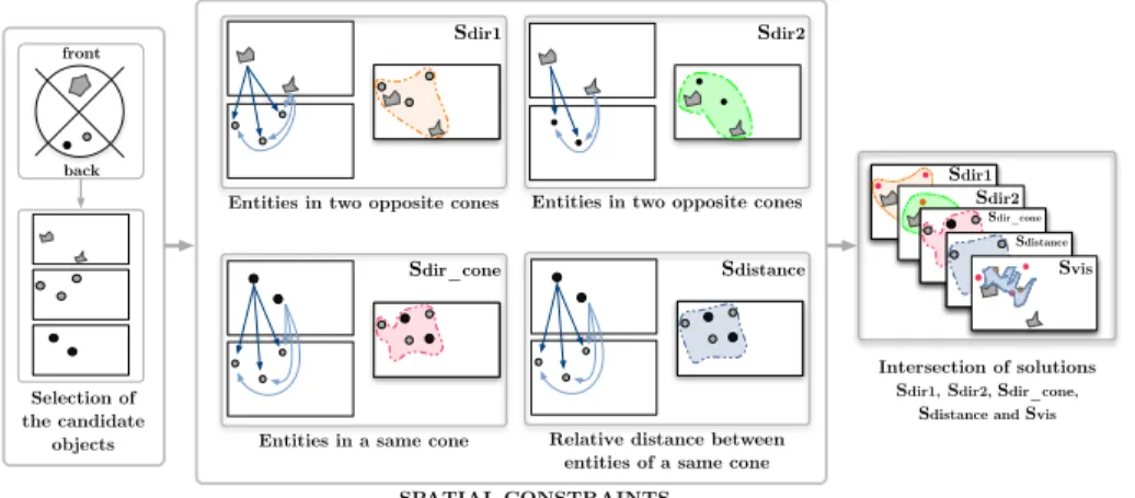
Overall, the final solution, i.e. the areas that correspond to the possible ob-server’s locations are given by the intersection of the solutions provided by each of these constraints. Since the geopositioning algorithm successively applies these complementary constraints, it significantly reduces the size of the solution space. Let us consider the spatial configuration given by the verbal description “ I am in front of a meadow and the castle is behind me. The drawbridge is behind the castle ” and illustrated by the conceptual map of figure 3. The application of the parser leads to the identification of three triplets, e.g., [meadow, in-front-of, observer], [castle, behind, observer] and [drawbridge, behind, castle]. The
visibil-ity algorithm identifies a first solution region Svisand the corresponding object
candidates. Four spatial constraints emerge from the previous example and are applied to each candidate object:
– the first case where entities are in opposite directional cones is applied both on pairs (“meadow”, “castle”) and (“meadow”, “drawbridge”).
– the second case where entities are in an identical cone is applied on the pair (“castle”, “drawbridge”).
– the third case that characterizes a distance relations between entities of a same cone is applied on the pair (“castle”, “drawbridge”).
Consequently, four possibles solution spaces Sdir_1, Sdir_2, Sdir_cone and
Sdistance emerge. The final solution is given by their intersection including the
previous solution Svis (Fig. 9).
Intersection of solutions Sdir1, Sdir2, Sdir_cone,
Sdistance and Svis
Sdir1 Selection of the candidate objects front back
Entities in two opposite cones Entities in two opposite cones Sdir2
Sdir1
Entities in a same cone Sdir_cone
Relative distance between entities of a same cone
Sdistance Sdir2 Sdir_cone Sdistance Svis SPATIAL CONSTRAINTS
Fig. 9. Constraint-based approach
4
Conclusion
Early models of geopositioning processes have been widely influenced by quan-titative representations of space. However, these approaches do not completely
reflect the way humans perceive and describe their environment since they prefer-ably process qualitative information. This paper introduces a method for geopo-sitioning an observer from the verbal description of his/her surroundings. A constraint-satisfaction algorithm is applied by successively refining the candidate locations of the observer. The first case of the approach considers some visibility constraints on the entities identified in the verbal description with respect to some candidate objects of the geographical database. The second case consid-ers direction and distance relations as spatial constraints, i.e. relative directions between entities and the observer, as well as distance relations are interpreted. Overall the geopositioning approach provides a set of possible locations for the observer. The algorithm still deserves integration of additional spatial relations, such as non-visibility constraints that can be derived from entities and land-marks not identified by the observer, but present in the geographical database. The approach is currently being implemented as an extension of the GvSIG software.
References
1. Herskovits, A.: Language and Spatial Cognition: An Interdisciplinary Study of the Prepositions in English. Cambridge University Press (1986)
2. Tversky, B., Lee, P.U.: How space structures language. Spatial Cognition: An In-terdisciplinary Approach to Representing and Processing Spatial Knowledge 1404 (1998) 157–175
3. Kuipers, B.: Modeling spatial knowledge. Cognitive Science 2(2) (April–June 1978) 129–153
4. Freksa, C.: Using Orientation Information for Qualitative Spatial Reasoning. In Frank, A.U., Campari, I., Formentini, U., eds.: Proceedings of the International Conference GIS - From Space to Territory: Theories and Methods of Spatio-Temporal Reasoning on Theories and Methods of Spatio-Spatio-Temporal Reasoning in Geographic Space. Volume 639 of LNCS., Springer Heidelberg (1992) 162–178 5. Smith, B., Mark, D.: Geographical categories: An ontological investigation.
Inter-national Journal of Geographical Information Science 15(7) (October 2001) 591– 612
6. Le Yaouanc, J.M., Saux, E., Claramunt, C.: A semantic and language-based rep-resentation of an environmental scene. GeoInformatica 14(3) (2010) 333–352 7. Montello, D.: Scale and multiple psychologies of space. In Frank, A.U., Campari,
I., eds.: Spatial Information Theory: A Theoretical Basis for GIS. Volume 716 of LNCS., Springer Heidelberg (September 1993) 312–321
8. Peuquet, D.J., Ci-Xiang, Z.: An algorithm to determine the directional relation-ship between arbitrarily-shaped polygons in the plane. Pattern Recognition 20(1) (1987) 65–74
9. Grice, H.: Logic and conversation. Syntax and Semantics 3(S 41) (1975) 58 10. Ligozat, G., Nowak, J., Schmitt, D.: From language to pictorial representations. In
Poznańskie, W., ed.: Proc. of the Language and Technology Conference, Poznan, Poland (September 2007)
11. Le Yaouanc, J.M., Saux, E., Claramunt, C.: A salience-based approach for the modeling of landscape descriptions. In Agrawal, D., Lu, C.T., Wolfson, O., eds.: Proceedings of the 17th ACM SIGSPATIAL International Conference on Advances in Geographic Information Systems, ACM Press (2009) 396–399
12. Cornell, E.H., Hill, K.A.: The problem of lost children. In: Children and their Environments: Learning, Using, and Designing Spaces. Cambridge University Press (2005) 26–41
13. Heth, C.D., Cornell, E.H.: A Geographic Information System for Managing Search for Lost Persons. In: Applied Spatial Cognition: From Research to Cognitive Tech-nology. Lawrence Erlbaum Associates (2006)
14. Ferguson, D.: GIS for wilderness search and recue. In: Proceedings of ESRI Federal User Conference. (2008)
15. De Floriani, L., Marzano, P., Puppo, E.: Line-of-sight communication on terrain models. International Journal of Geographic Information Systems 8(4) (1994) 329–342
16. Fisher, P.F.: Extending the applicability of viewsheds in landscape planning. Pho-togrammetric Engineering & Remote Sensing 62(11) (1996) 1297–1302
17. Fogliaroni, P., Wallgrün, J.O., Clementini, E., Tarquini, F., Wolter, D.: A qual-itative approach to localization and navigation based on visibility information. In Heidelberg, S.B.., ed.: Proceedings of the International Conference on Spatial Information Theory. Volume 5756. (2009) 312–329
18. De Floriani, L., Magillo, P.: Algorithms for visibility computation on terrains: a survey. Environment and Planning B (Planning and Design) 30(5) (2003) 709 – 728
19. Lee, J.: Analyses of visibility sites on topographic surfaces. International Journal of Geographic Information Systems 5 (1991) 413–429
20. Smardon, R.C., Palmer, J.F.: Foundations for Visual Project Analysis. Wiley and Sons, Inc (1986)
21. Travis, M.R., Elsner, G.H., Iverson, W.D., Johnson, C.G.: VIEWIT: computation of seen areas, slope, and aspect for land-use planning. Technical Report GTR-PSW-011, Berkeley, CA: Pacific Southwest Research Station, Forest Service, U.S. Department of Agriculture (1975)
22. Larive, M., Dupuy, Y., Gaildrat, V.: Automatic generation of urban zones. In Kunii, T.L., Skala, V., eds.: Proceedings of Computer Graphics, Visualization and Computer Vision. (2005)
23. AAkerberg, O., Svensson, H., Schulz, B., Nugues, P.: CarSim: an automatic 3D text-to-scene conversion system applied to road accident reports. In Copestake, A., Hajic, J., eds.: Proceedings of the tenth conference on European chapter of the Association for Computational Linguistics. Volume 2., ACM Press (2003) 191–194 24. Le Roux, O., Gaildrat, V., Caubet, R.: Using Constraint Satisfaction Techniques in Declarative Modelling. In: Geometric Modeling: Techniques, Applications, Systems and Tools. Springer (2004) 1–20
25. Desmontils, E.: Expressing constraint satisfaction problems in declarative modeling using natural language and fuzzy sets. Computers and Graphics 4(24) (2000) 555– 568
26. Mukerjee, A.: A representation for modeling functional knowledge in geometric structures. In Ramani, S., Chandrasekar, R., Anjaneyulu, K.S.R., eds.: Knowledge Based Computer Systems. LNCS, Springer Heidelberg (1990) 192–202
27. Levinson, S.: Frames of reference and Molyneux’s question: cross-linguistic evi-dence. Language and Space (1996) 109–169
![Fig. 1. Conceptual map of a scene [6]](https://thumb-eu.123doks.com/thumbv2/123doknet/7287448.208036/5.918.235.666.204.740/fig-conceptual-map-of-a-scene.webp)