HAL Id: hal-01760294
https://hal.archives-ouvertes.fr/hal-01760294
Submitted on 5 Mar 2019HAL is a multi-disciplinary open access
archive for the deposit and dissemination of sci-entific research documents, whether they are pub-lished or not. The documents may come from teaching and research institutions in France or abroad, or from public or private research centers.
L’archive ouverte pluridisciplinaire HAL, est destinée au dépôt et à la diffusion de documents scientifiques de niveau recherche, publiés ou non, émanant des établissements d’enseignement et de recherche français ou étrangers, des laboratoires publics ou privés.
BEM-based cooling channel optimization for 3D
injection molding
Nicolas Pirc, Florian Bugarin, Fabrice Schmidt, Marcel Mongeau
To cite this version:
Nicolas Pirc, Florian Bugarin, Fabrice Schmidt, Marcel Mongeau. BEM-based cooling channel opti-mization for 3D injection molding. 1st International conference on multidisciplinary design optimiza-tion and applicaoptimiza-tion, Apr 2007, Besançon, France. 6 p. �hal-01760294�
3D BEM-based cooling-channel shape optimization for
injection molding processes
N. Pirc*a, F. Bugarin*, F.M. Schmidt*, M. Mongeaua (*)CROMeP - Ecole des Mines d’Albi-Carmaux, Campus Jarlard, 81013 Albi, cedex 9, France
(a)LAAS-CNRS, Universit´e de Toulouse and
Institut de Math´ematiques, Universit´e Paul Sabatier 31062 Toulouse cedex 9, France
Abstract
Today, around 30 % of manufactured plastic goods rely on injection molding. The cooling time can represents more than 70 % of the injection cycle. Moreover, in order to avoid defects in the manufactured plastic parts, the temperature in the mold must be homogeneous. We propose in this paper a practical methodology to optimize both the position and the shape of the cooling channels in 3D injection molding processes. For the evaluation of the temperature required both by the objective and the constraint functions, we must solve 3D heat-transfer problems via numerical simulation. We solve the heat-transfer problem using Boundary Element Method (BEM). This yields a reduction of the dimension of the computational space from 3D to 2D, avoiding full 3D remeshing: only the surface of the cooling channels needs to be remeshed at each evaluation required by the optimization algorithm. We propose a general optimization model that attempts at minimizing the desired overall low temperature of the plastic-part surface subject to constraints imposing homogeneity of the temperature. Encouraging preliminary results on two semi-industrial plastic parts show that our optimization methodology is viable.
1
INTRODUCTION
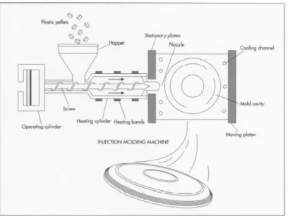
Today, around 30 % of manufactured plastic goods rely on injection molding, which is based on the injection of a fluid plastic material into a closed mold (Figure 1 [14] displays an illustrative injection molding process). The cooling time can represent more than 70 % of the injection cycle. Moreover, in order to avoid defects in the manufactured plastic parts, the temperature in the mold must be homogeneous. Thus, the design and the position of the cooling channels are crucial elements in the design of the mold. In order to decide the position and the shape of the cooling channels in the mold, designers commonly rely on experience and intuition within a costly trial-and-error design process. This manual design process becomes inadequate and unpractical for complex problems. This is particularly true nowadays with rapid prototyping processes such as layered design or selective laser sintering that enable manufacturers to build almost any desired shape of cooling channel geometry in the mold. As a consequence, designers need a more
power-1 INTRODUCTION
ful tool integrating the cooling analysis, its numerical simulation, and even optimization algorithms into the design process.
Figure 1: Temperature at the surface of the mold versus time
We propose in this paper a practical methodology to optimize both the position and the shape of the cooling channels in 3D injection molding processes.
For the evaluation of the temperature, required both by the objective and the constraint functions, we must solve 3D heat-transfer problems via numerical simulation. Severe numerical methods such as Finite Element Method (FEM) [1] or Boundary Ele-ment Method (BEM) [2] can be used for solving the heat-transfer problem. Silva [3] used 3D FEM software to model the injection molding cycle for complex geometries of molds. However, the computational burden of 3D FEM makes the integration of an optimiza-tion algorithm unpractical. Indeed, a FEM approach to the 3D heat-transfer problem imposes severe storage and CPU requirements, even if moderately complex industrial parts were to be targeted. An optimization algorithm requires numerous (and here ex-pensive in CPU time) objective-function evaluations. Moreover, unless one knows a very good initial design, from one optimization iteration to the next the design is generally significally different. As a consequence, the capability of FEM to handle (small) shape perturbations for 3D mesh cannot be advantageously exploited here. BEM is a method that was popularized by Brebbia [6]. It is used in many applications, such as gas-assisted injection molding processes [4], or groundwater flow and mass transport problems [5]. BEM transforms domain integrals into boundary element integrals, involving therefore a discretization restricted only to the external and internal field boundary. An optimization method can therefore be envisaged to modify the position and also the shape parameters of the cooling channels in order to improve the cooling performance of the mold.
2 THE HEAT TRANSFER PROBLEM
Park [7] proposed such a BEM-based procedure for the position of the cooling channels relying on augmented-Lagrangian optimization method. However, his study is restricted to molds that are generalized cylinders, amenable to 2D molds. His optimization model minimizes the variations of the temperature distribution on the cavity surface with re-spect to the average temperature. As a consequence, his optimal configuration provides a uniform but high average temperature, leading a very long cooling time which is not desirable in the context of large-scale manufacturing. Mathey [8] also used BEM to solve the heat-transfer problems with a Sequential Quadratic Programming (SQP) [9] algo-rithm to improve mold injection cooling. She minimizes an objective function which is the weighted sum of two criteria. Her first criterion is the average temperature at the plastic-part surface. Her second criterion is the sum of the temperature variations with respect to the average temperature. Moreover, Mathey optimizes both the position and the shape of the cooling channels. However, her approach is also restricted to 2D molds (as for Park, BEM then reduces the dimension of the computation space from 2D to 1D).
Our contribution is threefold. First, we address 3D mold geometries with a BEM approach reducing the dimension of the computation space from 3D to 2D, avoiding full 3D remeshing: only the surface of the cooling channels needs to be re-meshed at each evaluation required by the optimization algorithm. Secondly, we propose a general op-timization models that attempts at minimizing the desired overall low temperature of the plastic-part surface subject to constraints imposing homogeneity of the temperature. Thirdly, we demonstrate that our optimization methodology is viable with encouraging preliminary results on two semi-industrial plastic parts.
The paper is organized as follows. We detail in the next section the 3D heat-transfer problem that we must solve for every optimization evaluation of the temperature required by the optimization algorithm. Section 3 describes our overall optimization methodology. In order to validate our approach, we report encouraging preliminary results in Section 4. We conclude in Section 5.
2
THE HEAT TRANSFER PROBLEM
This section describes the heat-transfer problem that must be solved at every tem-perature evaluation required by the optimization algorithm:
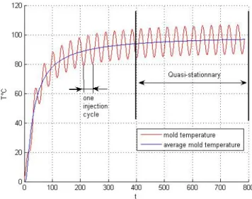
As shown in Figure 2 [10], after a few cycles the variation of the temperature in the injection mold in production can be considered to be quasi-stationary. Once the average temperature of the mold is stabilized, the cycle-averaged approach can predict well the overall performance of the cooling system. Thus, we can consider a stationary regime neglecting the transitory oscillations of the temperature.
2 THE HEAT TRANSFER PROBLEM
Figure 2: Temperature at the surface of the mold versus time
For a metallic mold, when between 0◦C to 200◦C, the thermal conductivity can be considered as a constant. Thus, the stationary heat conduction problem reduces to the following Laplace equation:
∆T = 0,
where ∆ is the Laplacian operator, T is a temperature vector. Multiplying this equa-tion by a weighting funcequa-tion T*, and using Green’s theorem, we obtain the well-known Somigliana’s equation [6]. The following Green integral representation formula gives the value of T in terms of integral equations involving the fundamental solution T* of the Laplace equation: C.T + Z Γ T.(∇T∗.n).dΓ = Z Γ (∇T.n).T∗.dΓ . (1) Here, n is the unit normal at one element, Γ is the boundary of the domain, C is equal to 1 inside the domain Ω and to 0.5 on its boundary Γ. The weighting function T ∗ and the flux q∗ are the fundamental solutions of the heat-problem, the so-called Green’s functions [6]: T∗ = −1 2.π.r and q ∗ = −r.n 4.π.r2 , (2)
where r is the distance from the point of application of the concentrated unit source to any other point under consideration. Note that in (1) all the integrals are taken over the boundary of the domain. For the computation of the heat-transfer problem, the contour Γ is discretized and the integrals in the above equation are defined in terms of nodal values by means of interpolation functions. After reorganization of terms in (2) using the boundary conditions, we obtain a non-symmetrical linear system. We shall need to remesh the cooling channel surfaces using 2D elements, and to solve this system of equations at every optimization evaluation.
2 THE HEAT TRANSFER PROBLEM
Figure 3: Boundary conditions
We detail the boundary conditions of the heat transfer problem in Figure (3). The following equation relates the temperature of the coolant, Tc, and the heat-transfer
coef-ficient, h, with the coolant flow rate (via Colburn correlation coefficient) [11]:
λ.q = h(Ta− Tc) ,
where λ is the conductivity, q is the heat flux, and Ta is the ambient temperature. The
following polymer properties are referenced in Table1: ρ is the density and Cp is the heat
capacity. The flux density at the cavity surface, φcavity, is computed from the cooling
cycle time, tcooling, and the polymer properties (heat due to polymer crystallization is
neglected) [11]:
φcavity =
Q tcooling.Γcavity
,
where Q is the heat evacuated by the plastic part during one injection cycle.
units polymer (PP) mold (steel 40cmd8s) λ W m−1 K−1 0.63 34
ρ kg m−1 891 7800 Cp J kg−1 K−1 2740 460
Table 1: Parameter values for heat-transfer problem
Finally, remark that for our problem, we only need to mesh once the cavity surface and the external surface of the mold. Then, each time the optimization algorithm re-quires to evaluate the objective and the constraint functions, we must mesh the surface of the cooling channels. The output of the heat-transfer problem resolution is a set of temperature measurements, one for each surface element: cavity, external mold surface, and cooling channels. However, we only need the vector T of temperature measurements, {Ti(x)}i∈S, at the cavity surface elements (S denotes the index set of the cavity surface
3 OVERALL OPTIMIZATION METHODOLOGY
3
OVERALL OPTIMIZATION METHODOLOGY
We first present in this section how we formulate our problem under a mathematical programming form. Then, we detail our overall computational methodology.
In the sequel, x will denote the vector of optimization variables (position and shape parameters for the cooling channels). Since the output of the heat-transfer problem is function of x, we shall make explicit the dependence of the temperature measurements upon the position and shape parameters x : {Ti(x)}i∈S.
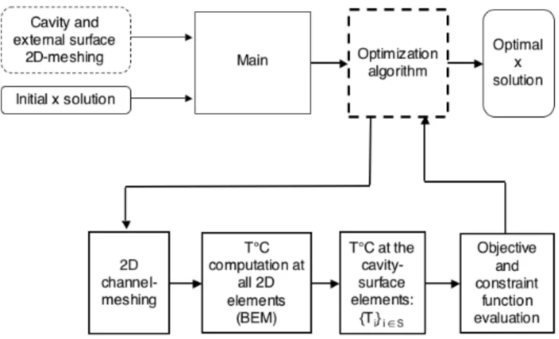
Figure 4: The heat-transfer simulation coupled with the optimization algorithm.
Most practical optimization problems involve several (often contradictory) ob-jective functions. It is the case here as one aims at minimizing the temperature of the plastic-part surface while minimizing the variation of the temperature along this surface. The simplest way to proceed in such a multicriterion context is to consider as objec-tive function a weighted sum of the various criteria, which involves choosing appropriate weighting parameter values (more on multicriterion optimization can be found in [15]). An obvious alternative is to use one criterion as objective function while requiring in constraints maximal threshold levels for the remaining criteria. We choose here the latter approach because in our application context, it is more desirable to consider the temper-ature requirement as a constraint. Indeed, we do know a threshold level value for the maximal temperature variation under which any variation is equally acceptable. More precisely, we formulate our problem under the form:
min
x kT (x)k
subject to f (T (x)) ≤ 0 (3)
g(x) ≤ 0, (4)
where f is a real-valued function used to stipulate the uniformity-temperature constraint, and g(x) is a general vector-valued non-linear function. Remark that k · k stands for any norm such as the l1 norm (sum of absolute values), the standard Euclidean (l2) norm, or
4 APPLICATIONS
the max (l∞) norm. The general constraints (4) represent any geometry-related or other
industrial constraints, such as:
• upper/lower-bound constraints on the xi’s,
• keeping the cooling channels within the mold,
• technically-forbidden zones where we cannot position the cooling channels (for in-stance due to the presence of ejectors),
• constraints stipulating a minimal distance between every pair of cooling channels to avoid inter-channels collision.
Figure4 shows the coupling between the thermal solver and the optimization algorithm.
4
APPLICATIONS
In this section, we present computational experiments on two semi-industrial plastic parts.
For both applications, we specify the following implementation strategies. We use com-mercial software for the tasks represented by dashed-line boxes in Figure 4:
• IDEAS for the initial 2D meshing of the cavity and the external surface (note that this meshing remains constant throughout the optimization process),
• Matlab’s fmincon [9] Sequential Quadratic Programming subroutine for the opti-mization algorithm (with finite-difference computation of the gradients for these preliminary experiments—in future work, we intend to compute exact gradients). We programmed every other task (represented by full-line boxes in Figure 4) in Matlab. The system of linear equations involved in the heat-transfer problem is solved by the LApack [16] subroutine included in Matlab 7.0. We use here the l∞ (max) norm for the
objective function:
kT (x)k∞:= max
i∈S Ti(x). (5)
All numerical results reported in the sequel are obtained on a Macintosh 1.83 GHz Intel core 2 duo.
4.1 EuroTooling mold with straight cooling channels
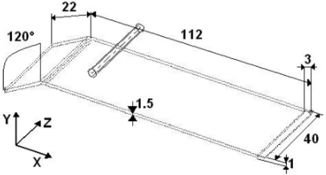
For our first application, we consider a semi-industrial injection mold design for the European project: EuroTooling 21 [17]. The plastic part produced from this mold is a bended plate whose dimensions are shown in Figure 5. We want to optimize the position of the cooling channels. The channels are simple straight horizontal cylinders of constant length as illustrated in Figure 6. In order to simplify the presentation, in this application we only optimize the position of the cylinders (we could also consider optimizing the radius of the cross-section of the channels and the number of channels, etc.). As a consequence,
4.1 EuroTooling mold with straight cooling channels 4 APPLICATIONS
three parameters suffice to describe the position of each cooling channel. For illustration purposes we consider here 8 cooling channels.
Figure 5: Plastic part dimensions and one cooling channel
Figure 6: Cooling channel parameters
The components of the optimization vector x are here the coordinates of each end point (Xi, Yi), i = 1 . . . 8. (in our application Zi is fixed). Thus, our problem
in-volves 16 optimization variables. For this application, we use the constraint function F (T (x)) = kT (x) − T (x)k∞− σ, where the difference T (x) − T (x) stands here for the
vector whose ith component is Ti(x) − T (x), T (x) := |S|1
X
i∈S
Ti(x) is the average of the
Ti’s, and σ is a user-defined temperature uniformity tolerance. We choose here σ = 4◦C.
In other words, we do not accept variations of the temperature that are above 4◦C with respect to the average temperature and this, everywhere on the plastic-part surface. The remaining constraints here simply stipulate lower/upper bounds and also forbid the grey zones displayed on Figure 6.
4.1 EuroTooling mold with straight cooling channels 4 APPLICATIONS
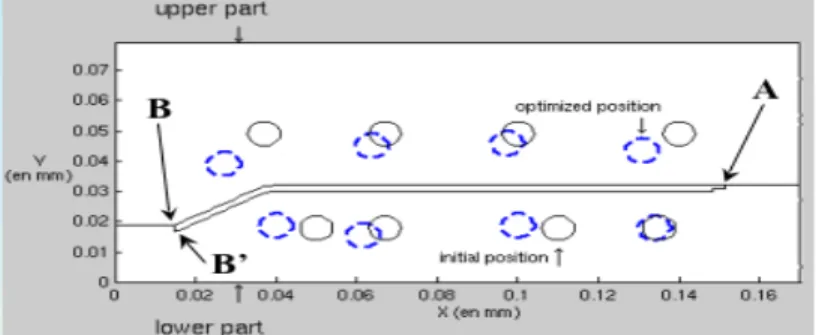
Figure 7: Initial and optimized (dashed lined) positions of the cooling channels
The 2D meshing of the mold surfaces is displayed in Figure 10. The surface of each channel is discretized into 320 quadrangles. We use as starting point, a heuristic solution provided by an experienced engineer. On average, one objective-function evaluation (i.e. the computation of the temperatures) requires 86 seconds of CPU time. Since for these preliminary experiments we are content with computing gradients using finite-difference approximations, one optimization iteration involves 26 minutes of CPU time on average. Figure 7 displays initial (full lines) and optimal (dashed lines) positions of the cooling channels. Figure8 displays the decrease of the objective-function value in terms of the number of optimization iterations. We observe on Figure 8that the objective function is reduced by 90% of its initial value within the first four optimization iterations.
Figure 8: Objective function versus iterations
Figure9shows the temperature distribution along the surface of the cavity mold before and after optimization (points A, B and B0 refer to positions on Figure 7). We observe that both the temperature variance and the average temperature decreased significantly. The temperature distribution after optimization can be seen on Figure 10
4.2 Plastic-cup mold with a helix cooling channel 4 APPLICATIONS
Figure 9: Temperature measurements along the surface of the mold cavity before (black) and after (grey) optimization
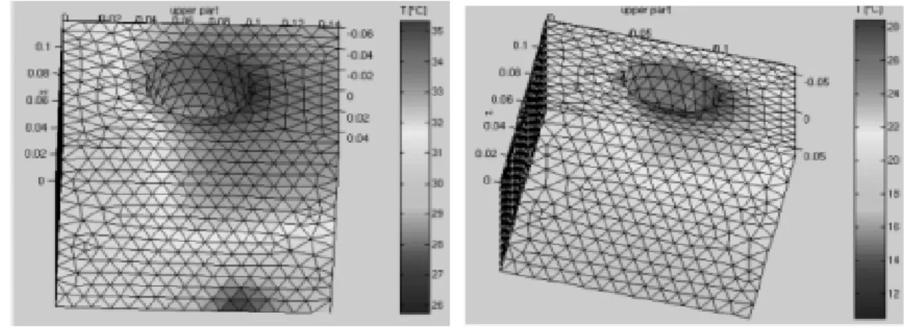
Figure 10: Temperature at the surface of the 3D mold after optimization
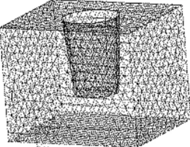
4.2 Plastic-cup mold with a helix cooling channel
We now report computational results on a 3D plastic part: a plastic cup. The height of the mold and that of the plastic cup are respectively 12 and 8 cm. The upper radius of the cup is 6 cm, its lower radius is 4 cm, and its thickness is 0.03 cm. In this preliminary study, we are content with considering a helix-shape cooling channel with circular cross section, with only three degrees of freedom: the section diameter of the cooling channel, the frequency of the turn and its overall diameter. The cooling channel is therefore defined in IR3 using the single parameter algebraic equation:
X(t) = rscos t
Y (t) = rssin t (6)
Z(t) = t ,
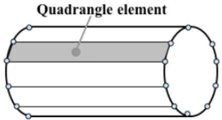
where rs is the radius of the spiral. We discretize this curve into 63 straight-cylinder
4.2 Plastic-cup mold with a helix cooling channel 4 APPLICATIONS
20 quadrangle elements as shown on Figure 13. The 2D meshing of the mold surfaces is displayed in Figure 11
The optimization variables here are:
• the geometrical parameters that control the shape of the helix, that is to say: the radius , rs of the spiral and the number, n, of helix turns,
• the radius rc of the circular cross section of the cylinder channels.
Figure 11: Meshing of the surfaces for the plastic-cup mold
4.2 Plastic-cup mold with a helix cooling channel 4 APPLICATIONS
Figure 13: Cooling-channel surface meshing
Our temperature homogeneity constraint here is:
max
i∈S Ti(x) − mini∈S Ti(x) ≤ σ,
with σ = 4◦C. The meshing of the mold surfaces is shown in Figure 12. On average, one objective-function evaluation (temperature computation) requires 82 seconds of CPU time. Again, because of the fact that we compute gradients using finite-difference ap-proximation, one optimization iteration involves, on average, 7 minutes of CPU time. Figure14 shows the helix curve before and after optimization.
Figure 14: Helix curve before (black) and after (grey) optimization
Figure15displays the decrease of the objective-function value in terms of the number of optimization iterations. We observe a rapid convergence during the first five iterations.
5 CONCLUSION
Figure 15: Objective-function value versus iterations
Table 2 displays the initial and optimal solutions, and Figure16 shows the tempera-ture distribution at the surface of the mold after optimization.
before optimization after optimization
rs (cm) 4.5 5.5
rc (cm) 0.3 0.1
n 10 5
objective-function value (◦C) 35◦C 28◦C max Ti− min Ti (◦C) 5 ◦C 2◦C
Table 2: initial and optimal solutions
Figure 16: Temperature at the surface of the 3D mold after optimization
5
CONCLUSION
We proposed in this paper a practical methodology to optimize both the position and the shape of the cooling channels in industrial 3D molds. This was made possible through the use of the boundary elements method that avoids full 3D remeshing. Indeed,
REFERENCES REFERENCES
only the surface of the cooling channels needs to be remeshed to solve the heat-transfer problem involved each time the optimization algorithm needs to evaluate the tempera-ture at the plastic part surface. Our optimization model can account for various ways to address the overall desired low-temperature criterion and the temperature-homogeneity constraint. Encouraging computational experiments on two semi-industrial plastic-parts, demonstrated the viability of our approach that is intended to be used as a decision-analysis tool for designing new, original mold geometries.
We are currently implementing exact gradients to replace finite-difference approximations in order to improve the efficiency of the optimization. Future work could allow more complex shape variations. Recall that we considered in this preliminary study only three degrees of freedom in order to test the viability of our optimization methodology. Other degrees of freedom for our plastic-cup application could for instance include the flux in the cooling channel and a vertical angle so that the helix runs along a cone (closer to the actual cup shape). Finally, further work could formulate our design problem as a topol-ogy optimization problem in order to offer even larger design freedom. The wide range of geometries we can tackle for the cooling channels will bring us to address more complex industrial molds. This will undoubtly yield challenging global optimization problems, as this can be anticipated based on the numerical experiments we reported.
Acknowledgments
This study was conducted within the framework of the European project EuroTooling 21 [17].
References
[1] Kolossov S., Boillat E., Glardon R., Fischer P. 3D FEM simulation for temperature evolution in the selective laser sintering process, International Journal of Machine Tools 44, 117-123, 2004. 2
[2] Polynkin A. Modeling of cycle 3D heat transfer in injection molding, International Polymer Processing XIX, 108-418, 2004. 2
[3] Silva L. In Parallel computation for solving efficiently 3D viscoelastic fluid flow prob-lems, International Polymer Processing XX, 265-273, 2005. 2
[4] Khayat K.E. In A three-dimensional boundary-element approach to gas-assisted injec-tion molding, Journal of Non-Newtonian Fluid Mechanics 57, 253-270, 1994. 2
[5] Katsifarakis K.L. In Combined use of BEM and genetic algorithms in groundwater flow and mass transport problems, Engineering Analysis with Boundary elements 23, 555-565, 1999. 2
[6] Brebbia C., Domiguez J. Boundary elements: An introductory course, WIT Press/Computational Mechanics Publication, 1992. 2, 4
REFERENCES REFERENCES
[7] Park S.J. Optimization method for steady conduction in special geometry using a BEM, International Journal for Numerical Methods in Engineering 43, 1109-1126, 1998. 3
[8] Mathey E. Automatic optimization of the cooling of injection mold based on the bound-ary element method, NumiForm, 222-227, 2004. 3
[9] J. Nocedal and S. S. J. Wright Numerical optimization, springer series in operation research, Springer, 1999. 3,7
[10] I. Catic, A. Abadzic and M. Rujnic-Sokele, Determining the optimum position of temperature sensors in molds for injection molding of polymers, Journal of Injection molding Technology, 3(4), 194-200, 1999. 3
[11] Jui-Ming L. Multi-objective optimization scheme for quality control in injection mold-ing, Journal of Injection molding Technology, 6 (4), 2002. 5
[12] The MathWorks, User’s Guide, Optimization Toolbox For Use With Matlab, Version 2, 2002.
[13] Wen-Hsien Y. Three-dimensional simulation of injection-compression molding of a compact disc, ANTEC 2001 Conference Proceedings, 2001.
[14] http://www.madehow.com/Volume-5/Frisbee.html 1
[15] Ehrgott M. Multicriteria Optimization, Springer, 2nd ed., 2005. 6
[16] LApack, http://www.netlib.org/lapack/ 7