Science Arts & Métiers (SAM)
is an open access repository that collects the work of Arts et Métiers Institute of Technology researchers and makes it freely available over the web where possible.
This is an author-deposited version published in: https://sam.ensam.eu
Handle ID: .http://hdl.handle.net/10985/10288
To cite this version :
Maxime GALLO, Kerem EGE, Marc REBILLAT, Jérôme ANTONI - A multi-sine sweep method for the characterization of weak non-linearities ; plant noise and variability estimation. - In: NOVEM 2015 _ Noise and Vibration Emerging Technologies, Croatie, 20150413 Noise and Vibration -Emerging Technologies - 2015
A MULTI-SINE SWEEP METHOD FOR THE
CHARACTERIZATION OF WEAK NON-LINEARITIES;
PLANT NOISE AND VARIABILITY ESTIMATION
M. Gallo1, K. Ege1*, M. Rébillat2 and J. Antoni1 1Laboratoire Vibrations Acoustique, INSA-Lyon,
25 bis, avenue Jean Capelle, F-69621 Villeurbanne Cedex, France Email:[email protected]
2Département d’études cognitives, Ecole Normale Supérieure Paris,
29 Rue d’Ulm, 75230 Paris, FRANCE Email:[email protected]
ABSTRACT
Weak non-linearities in vibrating structures can be characterized by a signal-model approach based on cascade of Hammerstein models. The experiment consists in exciting a device with a sine sweep at different levels, in order to assess the evolutions of non linearities on a wide fre-quency range. The method developed in [1], based on exponential sine sweep, is able to give an approximative identification of the Hammerstein models, but cannot make the distinction between nonlinear distortion and stationary plant noise. Therefore, this paper proposes improvements on the method that provide a more precise estimation of the Hammerstein models through the cancel-lation of the plant noise: it relies on the repetition of the signal on a certain amount of periods (multi-sine sweeps) and then on the consideration of the synchronous average out of the different periods from the resulting signal. Mathematical foundations and practical implementation of the method are discussed. The second main point of improvement concerning the study of the vibrating device is the use of the Bootstrap analysis. By considering some periods randomly chosen among the multisine sweep, one can study the variability of the experiments. The method becomes more robust.
1 INTRODUCTION
Many structures are generally assumed to undergo linear vibrations when they are driven at low levels, as the transverse motion w remains in a smaller range than the plate thickness, which is in practice not perfectly the case. Also, as non linearities appear - to a certain point - at a lower
amplitude than the linear response, it seems fundamental to measure theses non linearities with precision. Therefore the aim is to estimate measurement noise, whether it come from electronics or instruments, and then extract it out of the resulting signal.
This paper is thus organized around on the improvements concerning the exponential sine sweep based method, mainly developed in the work of Rébillat et al. [1], in order to study non linear be-havior of vibrating devices. The method at stake is described in Sec. 2. Then, the noise estimation is developed in Sec. 3. Concerning the improvement of the method itself, a more precise estimation of the kernels of Hammerstein models is discussed in Sec. 4. Also, the uncertainty measurement is presented through the Bootstrap procedure in Sec. 5. The obtained results on a vibrating plate are finally given in Sec. 6.
2 THE SINE SWEEP METHOD 2.1 Mathematical foundations 2.1.1 Cascade of Hammerstein models
Volterra series are a convenient tool to express analytically the relationship between the input e(t) and the output s(t) of a weakly non-linear system [2] which is fully characterized by the knowledge of its Volterra Kernels in the frequency domain {Vk(f1, · · · , fk)}k∈N∗. Cascade of Hammerstein
models constitute an interesting subclass of Volterra systems whose Kernels possess the following property:
∀k, ∃ ˜Vk: ∀(f1, · · · , fk), Vk(f1, · · · , fk) = ˜Vk(f1+ · · · + fk) (1)
Volterra Kernels of cascade of Hammerstein models can thus be expressed as functions of only one frequency variable and are in practice easy to estimate experimentally [1, 3]. This simple method is based on a phase property of exponential sine sweeps and the Kernels of such a model can be estimated from only one measured response of the system.
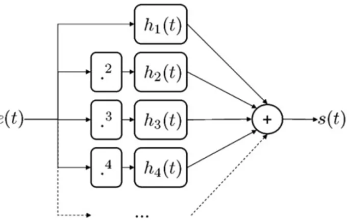
In a cascade of Hammerstein models [4], each branch is composed of one non linear static polynomial element followed by a linear one hn(t), as shown fig.1. Mathematically, the relation
between the input e(t) and the output s(t) of such a system is given by Eq. 2 ,where ∗ denotes the convolution: s(t) = N X n=1 (hn∗ e)n(t) (2)
In this model, each impulse response hn(t) is convolved with the input signal elevated to its nth
power and the output s(t) is the sum of these convolutions. The first impulse response h1(t)
rep-resents the linear response of the system. The other impulse responses {hn(t)}n∈{2···N }model the
non linearities. The family {hn(t)}n∈{1···N }will be referred to as the Kernels of the model. These
Kernels are assumed to be integrable. Any cascade of Hammerstein models is fully represented by its Kernels.
As can be seen in Eq. 2, cascade of Hammerstein models are linear in the parameters to be estimated, i.e. the output of the system is a linear combination of the Kernels {hn(t)}n∈{1···N }.
The method studied here gives direct mathematical access to all the Kernels {hn(t)}n∈{1···N }
from the contributions of the different orders of non linearity obtained as in Ref. [5]. The main advantage of the proposed approach is that it provides a direct evaluation of the N impulse re-sponses hn(t) of the system. The foundations and the key implementation of this simple method
are explained in detail in [1], where the whole procedure is validated on a simulated system and on two real systems.
Figure 1: Block diagram, representation of a cascade of Hammerstein models 2.1.2 Exponential sine sweeps
Estimating each kernel hn(t) of a cascade of Hammerstein models is not a straightforward task. A
simple estimation method that has been proposed previously by the authors [1] for this purpose is briefly recalled here. To experimentally cover the frequency range over which the system under study has to be identified, cosines with time-varying frequencies are commonly used. When the instantaneous frequency of e(t) = cos[f (t)] is increasing exponentially from f1 to f2 in a time
interval T , this signal is called an "Exponential Sine Sweep". It can be shown [1, 3] that by choosing Tm = (2mπ − π/2)ln(ff2 1)/2πf1 with m ∈ N ∗one obtains: ∀k ∈ N∗, cos(kφ(t + ∆tk)) with ∆tk = Tmlnk ln(f2 f1) (3) Eq. 3 states that for any exponential sine sweep of duration T , multiplying the phase by a factor k yields to the same signal, advanced in time by ∆tk.
2.1.3 Kernel recovery in the time domain
If an exponential sine sweep is presented at the input of a cascade of Hammerstein models, by combining Eq. 2 and Eq. 3 we obtain the following relation:
s(t) = N X n=1 (γn∗ e)n(t + ∆tn) with γn(t) = N X n=1 ck,nhk(t) (4)
where gn(t) is the contribution of the different kernels to the nth harmonic. In order to identify
each kernel hn(t) separately, a signal y(t) operating as the inverse of the input signal e(t) in the
convolution sense can be built as shown in [1]. After convolving the output of the cascade of Hammerstein models s(t) given in Eq. 4 with y(t), one obtains Eq. (4):
(y ∗ s)(t) =
N
X
n=1
γn(t + ∆tn) (5)
Because ∆tn ∝ ln(n) and f2 > f1, the higher the order of non-linearity n, the more advanced
is the corresponding γn(t). Thus, if Tm is chosen long enough, the different gn(t) do not overlap
in time and can be separated by simply windowing them in the time domain. Using Eq. 5, the family {hn(t)}n∈{1···N }of the kernels of the cascade of Hammerstein models under study can then
be fully extracted. Details of the computation of the matrix C are provided in [1].
2.2 An original method for detection of non linearities
The main advantage of this sine sweep based method is to be quick and simple; one can have direct access to the kernels of a vibrating device. However, this method needed to be improved to some extent. The main problem was the impossibility to make the difference between non linearities and the experimental noise, which resulted in an overestimation of the non linear behavior. Also, in order to fit better to the mathematical model, the number of kernels taken into account to describe the behavior of the vibrating device had to be more precise. Finally, in order to study the vibrating plate through the "Sweep" method, a simple tool was implemented to the previous method to provides the user with an indicator of the variability on the experimentations.
3 NOISE ESTIMATION
The multi-sine sweep described here is basically a signal containing the repetition of the exact same sweep. The sweep is defined by a starting frequency, an ending frequency and a time laps.
In the sweep-based method developed in [1], the input signal is a single sweep. The main hypothesis relies on the fact that the experimental noise follows a stochastic pattern. Therefore the aim to take the average out of the multi sine sweep from the result signal.
3.1 Mathematical foundations
The signal can be defined as the sum of response of the system s and the experimental noise n :
x(t) = s(t) + n(t) (7)
For a number K of exact same sweep of period T , the synchronous average corresponds to:
¯ s(t) = 1 K K−1 X k=0 [x(t − kT )] (8)
The noise can then be estimated by: ¯
n(t) = x(t) − ¯s(t) (9)
Finally, the signal to noise ratio (SNR) is:
SNR = 20 · log10(
RM S(s)
RM S(n)) (10)
3.2 Experimental validation
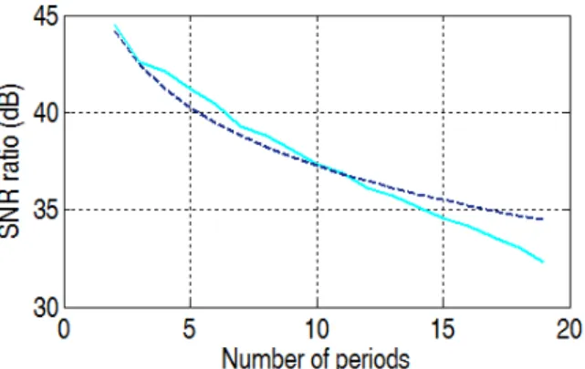
We can see on figure 2 the SNR levels of the result of different experiments, in comparison with the theoretical curve:
y = SNR(2) + 3 · ln2(2/N ) (11)
Experimental curves are likely to follow the same pattern as the theoretical one: a decrease of 3 dB as one double the number of repetitions.
3.3 Noise canceling and SNR Indicator
Once the noise is extracted from the result signal, it becomes then possible to assess the signal to noise ratio (SNR) of the experiment. This ratio gives one a precise indication on the validity of the experiments. The signal applied to the vibrating device must not be too low, in order to avoid the amplitude of the experimental noise reaching the amplitude of the global signal. However,
Figure 2: Multi sine sweep (- -) compared to the theoretical curve (—) the SNR ratio correspond here to the ratio between the RMS amplitude of the signal on the extracted RMS amplitude of the
noise.
a great SNR ratio also means important displacement, which involve chaotic behavior from the plate, instead of being weakly non linear; the model would become false.
4 SETTING OF THE RIGHT NUMBER OF KERNELS
The previous method could estimate a certain number of kernels. This number had to be defined by the user and could be wrong. Actually, a too small number of kernels taken into account resulted in a severe misunderstanding of the non linearities of the vibrating device. This is due to the fact that the lower kernels are depending on the higher ones. On the other side, a too big number of kernels implicated to consider experimental noise as a kernel.
Therefore, the procedure has to be autonomous, in its way of assessing the right number of kernels called Nopt. Hence the idea of having the computer estimating a great number of kernels, and to compare the RMS level of each of the estimated kernels. Once the procedure detects that the RMS level of a certain kernel do not reach the RMS level of experimental noise, this kernel must not be taken into account, and the method only study kernels from lower orders.
5 UNCERTAINTY OF MEASUREMENT 5.1 Statistical analysis of the experience
For a multi sine sweep of K periods, one does B random draws with replacement of K periods among the original K periods. For each value b (b = 1...B) the procedure calculates the syn-chronous average over the K periods randomly chosen. Then the B signals are implemented in the procedure in order to obtain different kernels. One gets then B number of each of the kernels estimated.
The idea then is to evaluate the accuracy of the experiments by calculating the synchronous average for each kernel, and then the confidence interval.
5.2 A more robust method
By synthetically increasing the number of experiments, one can assess the device behavior in a more reasonable time, as the Bootstrap implementation is not a really time consuming. Thus, this
procedure provides the user with a more accurate view on the non linear behavior of the device under study.
6 APPLICATION TO A VIBRATING PLATE
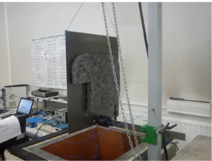
Figure 3: Steel plate excited with a shaker.
The device under study is a 1mm steel plate (see fig. 3), in free boundaries conditions. A shaker glued to the plate excites the plate with a multi sine sweep. In order to damp the system, a foam sheet was added to the plate.
6.1 Noise estimation and canceling
Fig. 4 shows how the noise perturbs the signal. This comparison between few random periods chosen among the result signal and the synchronous averaged signal gives a precise view on the spectral density of the stochastic noise; it is mainly present in the mid-frequencies.
Also, canceling the noise from the signal provides one with the certainty that resonance peaks really are a vibrating issue, and not a low quality power supply problems. The cancellation of the noise in the experimental signal is particularly important for the assessment of high orders kernels, which are very sensitive to noise due to there low level.
6.2 SNR indicator and setting of the right number of kernels
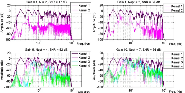
As depicted on fig. 5 non linearities level increases so as the global gain of the input signal. From a very low gain where the plate barely vibrates to great displacements (higher than the plate’s thick-ness) where non linearities level reaches linear level, one can observe several things concerning the improvements of the method. First, SNR is increasing as long as the input gain increases. In this case, SNR should be between 35 dB and 45 dB, so that the non linear response is comparable to the linear response, considering a weakly non linear behavior. Secondly, the method is now able to adapt to any situation, taking the right number of kernels into account. This number is getting bigger so as the input gain.
Figure 4: Frequency response of the system (linear part) without noise (—) (synchronous averaging) and with noise (—):1 period randomly chosen from the signal.
Figure 5: Hammerstein kernels for different amplitudes. Nopt is the optimal number of kernels calculated by the method.
6.3 Uncertainty of measurement
One can see on fig. 6 the application of the Bootstrap analysis on an experimental signal. Thanks to the Bootstrap procedure, the user is now able to detect artefacts in the experimental signal, particularly in mid-frequencies. This point is very important in the case of experiments in noisy environment.
7 CONCLUSION AND PERSPECTIVES
In this article an original vibro-acoustical method is presented to assess the proportion of non-linearities among the resulting signal. This method, based on a sine sweep, is able to assess whether the vibrating device behaves linearly or not. Moreover, the repetition of the same sweep
Figure 6: Frequency response of the system (linear part) with 10 Bootstrap samples. signal considerably improved the accuracy of the method, as it is now possible to extract noise from the resulting signal, and then to estimate the signal to noise ratio (SNR). The Bootstrap analysis really enhanced the view on the frequency response of the vibrating plate. The improvements on the method developed by Rébillat et al. [1] now provides the user with a more precise tool to study vibration and acoustic response of a vibrating device. The experiments being now K times longer (with K the number of periods of the multi sine sweep) than before, a next step would be to find a compromise between accuracy and time consuming.
8 ACKNOWLEDGMENTS
Since 2011, the Laboratoire Vibrations Acoustique is part of the LabEx CeLyA of Université de Lyon, operated by the French National Research Agency (ANR-10-LABX-0060/ ANR-11-IDEX-0007).
REFERENCES
[1] M. Rébillat, R. Hennequin, E. Corteel, and B. F.G. Katz. Identification of cascade of hammer-stein models for the description of nonlinearities in vibrating devices. Journal of sound and vibration, 330:1018–1038, 2011.
[2] S. Boyd and L. O. Chua. Fading memory and the problem of approximating nonlinear opera-tors with volterra series. IEEE Transactions on Circuits and Systems, volume = 32(11), pages = 1150-1161, year = 1985.
[3] A. Novak, P. Lotton, L. Simon, and F. Kadlec. Modeling of non linear audio systems using swept-sine signals: application to audio effects. 12th Int. Conference on Digital Audio Effects (DAFx-09, Paper 5093, September 2009.
[4] P.G.Gallman. Iterative method for identification of non linear - systems using a uryson model. IEEE Transactions on Automatic Control, volume = 6, pages = 771-775, year = 1975.
[5] A. Farina. Simultaneous measurement of impulse response and distorsion with a swept-sine technique. 108th Convention of the Audio Engineering Society, Paper 5093:2065–2075, febru-ary 2000.