TH `
ESE
TH `
ESE
En vue de l’obtention du
DOCTORAT DE L’UNIVERSIT ´
E DE TOULOUSE
D ´elivr ´e par : l’Universit ´e Toulouse 3 Paul Sabatier (UT3 Paul Sabatier)
Pr ´esent ´ee et soutenue le 04/12/2017 par :
K´
evin CILLEROS
Diversit ´e et r `egles d’assemblage des communaut ´es de
poissons d’eau douce de Guyane
JURY
N ´URIABONADA Associate Professor Rapporteuse
CATHERINEGRAHAM Full Professor Rapporteuse CHRISTOPHER BARALOTO Professeur Evaluateur
GAEL¨ GRENOUILLET Maˆıtre de conf ´erence Evaluateur
THIERRYOBERDORFF Directeur de recherche Evaluateur
S ´EBASTIEN BROSSE Professeur Directeur de th `ese
´
Ecole doctorale et sp ´ecialit ´e :
SEVAB : ´Ecologie, biodiversit ´e et ´evolution Unit ´e de Recherche :
´
Evolution et Diversit ´e Biologique (UMR 5174) Directeur de Th `ese :
S ´ebastien BROSSE (Professeur, Universit ´e de Toulouse III) Rapporteurs :
Diversity and assembly processes of
Guyanese freshwater fish assemblages
K ´evin CILLEROS
Jury composition
N ´uria BONADA Associate Professor Referee
Catherine GRAHAM Professor Referee
Christopher BARALOTO Professor Jury member
Ga ¨el GRENOUILLET Senior lecturer Jury member
Thierry OBERDORFF Researcher Jury member
S ´ebastien BROSSE Professor PhD supervisor
Defended on December 4, 2017
I would like to first thank the courageous readers that will take the time to read at least one part of this manuscript. I hope you will learn something or find what you were looking for within it.
My gratitude also goes to N ´uria and Catherine who accepted to review my work, and all the jury members. As the time of writing these words, I don’t know how things will happen but in every cases, I know that all your comments and your external view will be helpful to improve these works and get new research avenues.
La suite de mes remerciements (en franc¸ais) va au Centre d’Etude de la Biodiversit ´e Amazonienne qui a financ ´e cette th `ese et `a ces membres qui m’ont fait confiance pour mener ce projet `a son terme.
Pour rester sur la th ´ematique tropicale, je souhaite aussi remercier Damien Monchaux, Simon Clavier, Laurent Guillemet et Roland, membres d’HYDRECO, avec qui j’ai partag ´e une partie du travail de terrain en 2015 (et ma premi `ere pose de filet, mon premier voyage en pirogue, mon premier passage de saut). Merci aussi `a R ´egis Vigouroux pour son accueil et sa visite guid ´ee de Cayenne et Kourou.
Merci aussi Tony Dejean, Alice Valentini et Rapha ¨el Civade pour leur accueil au Bourget-du-Lac et les conseils concernant le metabarcoding.
Je remercie aussi Sarah Delavigne et Coline Gaboriaud, deux stagiaires qui ont particip ´e au d ´eveloppement des bases de donn ´ees morphologiques et mol ´eculaires.
Huit ann ´ees sur le campus et quatre ans pass ´ees au laboratoire EDB, c’est aussi des ann ´ees pass ´es avec des personnes grandioses, des amis et une seconde famille. Je ne vais pas faire un inventaire exhaustif de ces personnes (il y en a bien assez dans la suite du texte) mais rapidement, je retiendrai la communaut ´e des r ´esidences Jean Mermoz et adjacentes (Cl ´ement, Marc, Romain, Julie, Marie, Adeline, Hugo), la communaut ´e M2 (Seb, Eva, Meli, Caroline, Lucie, Jan, Andrea et en particulier David et Chaton qui m’ont accueilli chez eux) et la communaut ´e doctorants et post-doctorants (Jade, C ´eline, Eline, Aurore, Carine, MC Solaire, F ´elix le chat, Fabian, Jess, Sandra, les petits nouveaux, les anciens d’EDB). Merci aux secondes mamans ou grandes sœurs Amaia, Catherine et Lucie Z., et aux grands rigolos, Pierrick et Guillaume, qui m’ont souvent fait rire.
Un gros bravo Jade qui a su trouver l’ ´energie de me supporter durant ces derni `eres ann ´ees, entre mes blagues qui ne faisaient rire que moi ou mes perp ´etuelles discussions avec moi m ˆeme. Bravo aussi `a Seb pour avoir tenu deux ans et demi.
Je tiens aussi `a remercier Linda, Catherine, Dominique, Nicole, aupr `es desquelles les questions administratives, financi `eres ou d’organisation ont su trouver des r ´eponses, et Pierre pour l’excellente assistance informatique (surtout quand l’ordinateur ne s’allume plus).
De l’autre c ˆot ´e du miroir du laboratoire, il y a une famille, sur laquelle j’ai toujours pu compter et dans laquelle j’ai pu me ressourcer lorsqu’il le fallait. Merci `a mes parents
Acknowledgements
pour le soutien qui m’a permis d’ ´etudier `a l’universit ´e.
Que serait des remerciements en bonne et due forme sans un mot aux personnes qui m’ont fait confiance tout au long de ces quatre ann ´ees: Ga ¨el et S ´ebastien. Cette aventure a commenc ´e par le stage de M2: mes r ´eels premiers pas dans le monde de la recherche. Puis la th `ese, une autre marque de confiance pour moi. Gr ˆace `a vous, j’ai pu aller dans des lieux o `u je n’aurais jamais pu aller. Ces ann ´ees de formation m’ont beaucoup apport ´e tant sur le c ˆot ´e professionnel (c’est un peu le but d’une th `ese non ?) que sur le c ˆot ´e personnel et surtout la confiance en soi.
Une petite pens ´ee pour les compositeurs et artistes qui ont berc ´e mes oreilles durant cette p ´eriode et particuli `erement sur cette fin de th `ese, en particulier Yoko Shimomura et Shoji Meguro. Ces ´ecrits ne les atteindront s ˆurement jamais, mais je suis arriv ´e jusque l `a gr ˆace `a eux aussi.
Chapter I: Introduction 11
I.1 Biodiversity: from pattern to process . . . 11
I.1.1 The historical roots of biological diversity . . . 11
I.1.2 The current definition of biodiversity . . . 11
I.1.3 Biodiversity at the community level . . . 12
I.1.4 The patterns of biodiversity . . . 13
I.1.5 A diversity of processes . . . 14
I.1.6 Unlocking the “Same pattern from several processes” problem . 19 I.2 Application to French Guiana freshwater fish assemblages . . . 25
I.2.1 The Guianese territory . . . 25
I.2.2 Guianese demography and anthropogenic activities . . . 25
I.2.3 History and biogeography . . . 26
I.2.4 Aquatic ecology . . . 26
I.3 Thesis . . . 28
I.3.1 Aim . . . 28
I.3.2 Taxonomic data: assemblage composition in streams and rivers . 28 I.3.3 Functional data: morphological measures and functional traits . . 30
I.3.4 Molecular data: molecular markers and phylogenetic relationship 33 I.3.5 Sites descriptors: environment and space . . . 33
I.3.6 Thesis conduct and structure . . . 34
Chapter II: Diversity of freshwater fish assemblages in undisturbed small streams 37 II.1 Summary . . . 37
II.2 Manuscript A: Disentangling spatial and environmental determinants of fish species richness and assemblage structure in Neotropical rainforest streams . . . 41
Chapter III: Assembly processes in Guianese freshwater fish assemblages 75 III.1 Assembly processes between temperate and tropical freshwater fish assemblage . . . 75
III.1.1 Summary . . . 75
III.1.2 Mansucript B: Taxonomic and functional diversity patterns reveal different processes shaping European and Amazonian stream fish assemblages . . . 78
Chapter IV: Toward a new sampling protocol: a molecular approach with
eDNA metabarcoding 123
IV.1 Summary . . . 123
IV.2 Manuscript C: Unlocking biodiversity and conservation studies in high diversity environments using environmental DNA (eDNA): a test with Guianese freshwater fishes . . . 126
IV.3 Additional analyses . . . 198
Chapter V: Conclusion 205 V.1 Assembly processes of Guianese freshwater assemblages . . . 205
V.2 Phylogenetic characteristics of assemblages . . . 205
V.3 Functional characteristics of assemblages . . . 206
V.4 Assembly processes and anthropogenic disturbances . . . 206
V.5 Leaving the “process from pattern” way of thinking? . . . 207
List of Figures 211
List of Tables 213
Glossary 215
Bibliography 217
I.1 Biodiversity: from pattern to process
I.1.1
The historical roots of biological diversity
Diversity, the range of variation in a set of features, has long been described for biological organisms. The first known written facts date back to Aristotle in his History of Animals (350 BCE). He recognized that some animals have the same characteristics, whereas others are different, both in their morphology (or in their “parts”, Aristotle, 1910) and in their behavior (“in their modes of subsistence, in their actions, in their habits”, Aristotle, 1910). This pioneering work of zoology has ruled, without improvment, until theXVIthcentury (Barth ´elemy-Saint-Hilaire, 1883), when two
French zoologists, Pierre Belon and Guillaume Rondelet, pursued Aristotle’s work and travelled around the Mediterranean Basin to describe plants and animals (especially aquatic animals; Belon, 1555; Rondelet, 1558). The next progresses occured during the XVIIIth century with the works of Carl Linnaeus, widely known for its biological
classification of organisms, which principles are still used in taxonomy. Georges L. Leclerc, Comte de Buffon, then linked observations and description of species with the history of Earth to explain some of the patterns he observed that set first principle in biogeography (Buffon’s Law that states that geographically isolated areas with similar environment have different species, Buffon, 1761). A tipping point occurred during the XIXth century, with the works of Charles Darwin, where the classical natural observational approach faded to the benefit of a more inductive or ‘scientific’ approach. From here, biological sciences benefited from the emergence of new fields (evolution, genetic, ecology) and the fortification of previous theories in biogeography (e.g. Alexander von Humboldt‘s or Alfred R. Wallace‘s works). However it was not until the second half of the XXth century that the term of “biological diversity” emerged from
the field of conservation biology. The term biological diversity was first used by Thomas Lovejoy (1980) to refers to species diversity in tropical forests, and its contraction into “biodiversity” appeared soon after, for the “National Forum on BioDiversity” in 1986 organized by Walter G. Rosen and the publication of the proceedings of this forum under the name “BioDiversity” (Wilson & Peter, 1988), then stared its popularity among scientists, politics and people.
I.1.2
The current definition of biodiversity
Biodiversity can be defined as “the variety of life, at all levels of organization, classified both by evolutionary (phylogenetic) and ecological (functional) criteria” (Colwell, 2012). Colwell’s definition of biodiversity can be decomposed into three parts. The first part, “the variety of life” is synonymous to biological diversity and does not inform much on what is understood when speaking about “life”. It’s the second element of the definition that explicit it: the expression “levels of organization” refers to the nested organization
Introduction
of life from genes to ecosystems. From this,“life” will have a different meaning at each of these levels. For example, the diversity of species at thecommunity or assemblage level is the most known descriptor of biodiversity. Biodiveristy can also be described at the gene level using the diversity of alleles or genes (genetic polymorphism), or at the population level with the diversity in individual genotypes and phenotypes. To determine those of biodiversity descriptors, Colwell’s definition lies on evolutionary and ecological characteristics. These characteristics have been commonly used to delineate species, but they can also apply to other levels of organization (genetic lineage, individuals, functional groups or landscapes).
I.1.3
Biodiversity at the community level
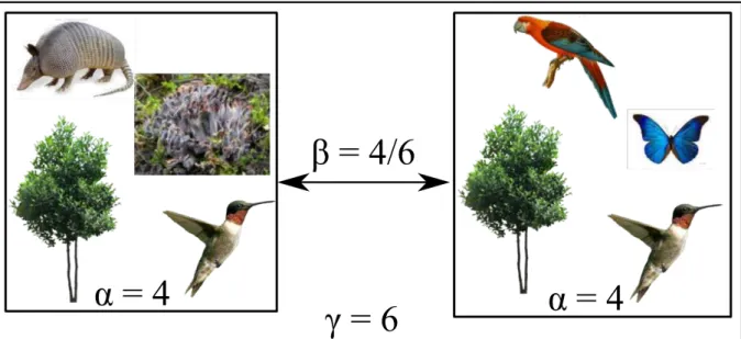
Using Colwell’s definition, species can be used as the unit of diversity at the community level. If we consider a set of communities, a first and simple diversity descriptor will be the list or number of species, also called species richness, in each community (Figure I.1). We can also look if all species have the same abundance in each community or if some species dominate the community. In this case, the equitability or evenness of the community is used as a descriptor of diversity. Together, species richness and equitability reflect community composition and represent community diversity.
These measures of community diversity apply to each community and represent within-community diversity, or α-diversity. Summarizing communities using their species richness and evenness allows comparisons across communities but does not detect potential differences in the species compositions between communities. For instance, in Figure I.1, the two communities have each 4 species (α-diversity = 4) but they do not share all their species (only two are shared). One way to deal with this is to compare communities and look at between-community diversity, or β-diversity. A classical measure of β-diversity is the percentage of species that are shared (or not shared) between communities (e.g. Jaccard, 1912 or Sørensen, 1948 indices). In the Figure I.1, the two communities have 2 species in common and 4 species are only found in one of the two communities. So, the diversity between the two communities is
4
6 ≈ 0.67. This value means that the two communities share about 33% of the total
number of species found in these communities. This type of metrics can be extended to several communities and some metrics were developed to take into account species abundances [Bray-Curtis (Bray & Curtis, 1957) or Manhattan measures (Michener & Sokal, 1957)].
Finally, we can look at the total diversity across all the communities or γ-diversity. It reflects information given by both α- and β-diversity measures. For example, if communities share a lot of species, the total diversity tends to be close to the maximal value of α-diversity. In contrast, γ-diversity will be high if each community has a unique set of species.
These terms of α-, β- and γ-diversity were firstly introduced by Whittaker (1960) and several definitions and metrics have followed (Whittaker, 1972; Anderson et al., 2011) but all converge towards the idea that within-, between- and total diversity
represent different facets of biodiversity, that provide complementary information to describe patterns of diversity.
Figure I.1: Biodiversity can be spatially decomposed in 3 levels: the diversity of a local assemblage
or habitat (α-diversity), the difference in diversity between two or more assemblages or habitats (β-diversity), and the total diversity of assemblages or habitats. In the example above, each community is composed of 4 different species (thus α-diversity = 4 for each). If we compare the 2 communities, we see that they share two species and each community has 2 unique species. The 2 communities thus share 2 species in common over 6 species, that is 26 ≈ 33%, and the diference in diversity between the two communities (β-divesity) is 1 − 26 = 46 ≈ 67%. In total, the diversity in these communities is equal to 6 species (γ-diversity)
I.1.4
The patterns of biodiversity
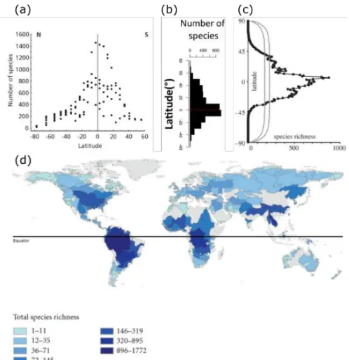
Diversity is not evenly distributed across the globe and thus exhibits spatial variability, from large to local spatial scales. At the global scale, the best studied biodiversity pattern is the latitudinal diversity gradient. Several authors have reported that a high number of species occur around the equator, and that their number decrease toward the poles, causing a hump shaped relationships between species richness and latitude (Figure I.2). This pattern is shared by most organisms (woody plants, birds, freshwater fish) despite some variability in the position of the peak of richness and the rate of richness decrease with increasing or decreasing latitude (Hillebrand, 2004). Diversity also differs between continents and regions for a same latitudinal range. For example, the number of freshwater fish species in South America is 1.3 times higher to that of Africa (L ´ev ˆeque et al., 2007). But the most striking difference between these regions is the difference in the identity of species. Such difference in species composition between regions is among the most striking biogeographical patterns, and was used to define the biogeographic realms in early biogeographic studies from the XIXth century (Wallace, 1876; Sclater, 1858; Engler, 1879). Within a region, local
diversity is also unequally distributed between the different ecosystems and habitat features, with patterns and gradients highly variable. Forest ecosystems do not have the same communities (group of directly or indirectly interacting species, co-occurring
Introduction
Figure I.2: The latitudinal diversity gradient is described in several taxa, from New World birds (a),
mammals (b), amphibians (c) and freshwater fishes (d). Figures from Gaston & Blackburn (2008), Rolland et al. (2014), Pyron et al. (2015) and Oberdorff et al. (2011) respectively
in space and time) and the same species richness as grassland ecosystems. In freshwater ecosystems, within a drainage basin, species richness increases from small upstream sites to large rivers and freshwater communities change along this gradient, with species associated to headwater streams and others endemic of large and deep channels (Huet’s zonation (1959) and River Continuum Concept from Vannote et al., 1980). Understanding what shape these patterns remains an outstanding key question in ecology and requires combining several research fields (phylobiogeography, niche and spatial modelling, evolutionary biology). The improvement of modeling techniques and the development of new methods and tools of have accompanied the rapid and vast gathering of biodiversity data (via automatic recording devices, high-throughput DNA sequencing, citizen science; Bush et al., 2017) and their availability through online databases [GBIF (http://gbif.org), GenBank (Benson et al., 2017), The Ocean Biogeographic Information System (Grassle, 2000)] allow to tackle this question.
I.1.5
A diversity of processes
The processes that shape the spatial patterns of biodiversity are scale dependent, although often not exclusive to a given spatial (or temporal) scale. A process that 14
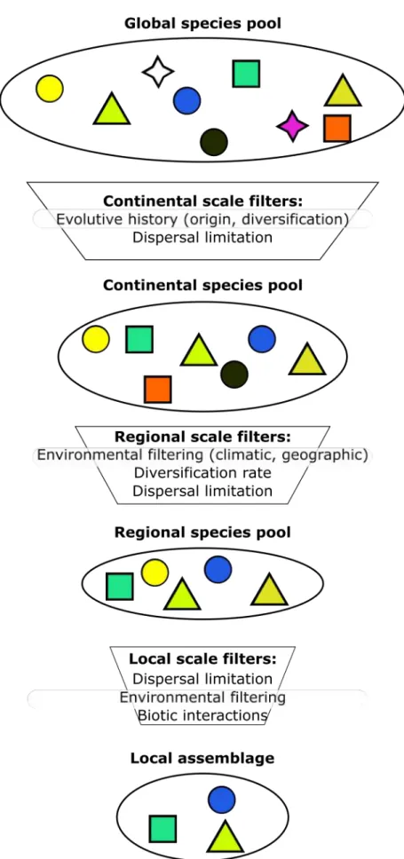
explains the global variation of species richness will therefore have a low influence on local diversity variation. For instance, the latitude is highly influential at the global scale, but it hardly affects local biodiversity variation. The reverse for more local processes also holds (e.g. interactions between species occur at a local scale and hardly affect diversity gradients measured at higher spatial scales). We can thus sort these processes according to the spatial scale considered. This led to formalize these processes as hierarchical filters (Tonn, 1990; Poff, 1997) acting at global, regional or local scales on a set of candidate species (orpool of species). Those filters therefore select the species occurring at a given scale from a set of potential species co-occurring at higher scales (Srivastava, 1999).
Global scale processes
At the global scale, four main non-exclusive groups of hypotheses have been proposed to explain the latitudinal diversity gradient (LDG).
First, the observed pattern might result from random distribution of species range along a latitudinal axis bounded at the two poles, without the need of any environmental effect. This geometric rule predicts that majority of species midpoint range will fall near the centre of the axis, corresponding to tropical regions (the mid-domain effect; Figure I.4, Colwell & Hurtt, 1994).
Aside from this neutral hypothesis, geographical differences between tropical and temperate regions can also contribute to the latitudinal diversity gradient. Tropical regions form a continuous entity, whereas temperate and polar regions are distributed part aside of it and form smaller entities. Larger areas are associated with higher species richness, through a greater speciation rate, a lower extinction rate and higher diversity of habitat (species-area relationship, Preston, 1962).
Tropical regions also receive higher solar radiation that can translate in higher primary productivity and in higher climatic stability and lower seasonality variability (Hutchinson, 1959; Hawkins & Porter, 2003; Currie et al., 2004). The species-energy relationship has been criticized because experimental studies showed that the species richness indeed increase with energy, but stops increasing or decreases after a threshold, and it thus might only be applicable under particular conditions (Hurlbert & Stegen, 2014).
A third group of hypotheses deals with the biogeographic historic differences between tropical and temperate regions, and associated evolutionary consequences. These hypotheses stipulate that diversity patterns are caused by differential speciation and extinction rates between tropical and temperate regions (Rolland et al., 2014). Two mechanisms have been proposed to explain those differences: either the tropical regions are older and more species originated from those areas (Wiens et al., 2011), or diversification rates are higher in the tropical regions compared to those observed in the temperate regions (Mittelbach et al., 2007; Pyron & Wiens, 2013). Some studies also suggested the existence of phylogenetic tropical niche conservatism, the tendency of tropical species to retain ecological traits related to
Introduction
Figure I.3: Processes structuring local assemblages. The processes can be considered as a succession
of filters that act at different spatial scales (continental, regional, local scales). Symbols represent species
Figure I.4: Illustration of the mid-domain effect with an analogy, where species range are represented
by pencils, enclosed in a bounded box. If pencil positions are randomly distributed, the expected number of overlapping pencils is greater in the middle of the box rather at its edges. Adapted from Colwell et al. (2016)
tropical environment (Wiens & Donoghue, 2004). This would limit their dispersal capacity to regions outside of the tropics (dispersal limitation). Recently, Morini `ere et al. (2016) proposed a similar mechanism for taxa that present inverse latitudinal gradients, based on temperate niche conservatism for lineages originating from temperate regions.
More recently, biotic interactions, although acting mainly at local scales, has regained importance as a mechanism that can affect global scale diversity patterns (Schemske et al., 2009; Pianka, 1966). The relative stability of the climate over geological times for tropical areas allows the establishment of numerous interactions between species. In addition, this stability makes the environment more predictable and therefore relaxes the strength of selection by abiotic factors. In contrast, abiotic environment is the main constraint to species evolution in temperate regions and its variability selects for more generalist species (Stevens, 1989). The shift from the dominance of abiotic constraints to the dominance of biotic constraints in tropical areas makes the opportunity for co-evolution to be a strong driver of speciation, where optimum phenotypes always change, facilitating adaptation and speciation Schemske et al., 2009; Pianka, 1966. Biotic interactions include the effect of competition that promotes speciation through niche specialization. It also includes predation, which strength in tropical ecosystems (due to the high number of predator species) can reduce the competitive exclusion of prey species and thus enhance diversity (Janzen, 1970; Connell, 1971).
Despite the apparent separation of geometrical, geographical, historical and biotic hypotheses, they are not exclusive and together contribute in shaping diversity at the global scale.
Regional scale processes
At the regional scale, the pool of species is constrained by biogeographic, climatic and geographic variations within the considered region. Similarly to the global processes, differences in diversification rates between regions caused by geologic events can
Introduction
cause difference in diversity between regions located under same latitudes. For example, ancient refuge areas during glaciation or marine incursion periods have higher species richness and endemism than other areas (Svenning & Skov, 2007; Lawes et al., 2007; Reyjol et al., 2007). Climatic and landscape features also restrict the identity of species that occur in a region. This combination of environmental characteristics and biotic component (the species present) have been used to define ecoregions (area with relative homogeneity of ecosystems), even if recent definitions put the emphasis more on the biotic component (Olson et al., 2001; Abell et al., 2008). Local scale processes
At the local scale, two kinds of processes, or assembly rules, have been proposed to determine diversity patterns, deterministic processes and neutral processes, which represent the two extremes of a spectrum.
Deterministic or niche-based processes put the emphasis on the role of abiotic and biotic environment on community composition that successively act on the species pool to define occurring species. First, species that can establish and persist under given abiotic conditions (e.g. climate, temperature, soil characteristic...) will constitute a potential set of species. This process is referred as environmental filtering. Then, biotic interactions between species will restrain this set of species to the observed occurring species. Traditionally, competition is considered as the main biotic constraint that will prevent species with similar ecology to co-occur (a process also called limiting similarity), but predation and facilitation also affect community composition. A first approach to make the distinction between abiotic and biotic constrains on species assemblages was through the use of the ratio between the number of genera found in a community and the number of species (Elton, 1946). A low species-to-genus ratio indicates that the community is composed of relatively distantly related species and is expected is limiting similarity is the dominant process. On the contrary, a higher ratio is expected under environmental filtering. Its use was however greatly criticized as it highly depends of the sample size, with the species-to-genus ratio increasing with an increasing number of species (Gotelli & Colwell, 2001; Jarvinen, 1982).
At the other end of the spectrum, the neutral processes root in Hubbells neutral theory (Hubbell, 2011) where all individuals and species are functionally equal, so the environment impacts them equally, and only dispersal capacity and survival affect community composition. It is a dynamic equilibrium between migration from the species pool to local communities and local ecological drift that shape the community composition. Proposed as an alternative to more deterministic models, neutral hypotheses are currently used as a null model to establish random expectations against which the observed patterns are tested. Differences between these expectations and the observed patterns are often interpreted as the sign of the effect of deterministic processes in community assembly.
I.1.6
Unlocking the “Same pattern from several processes”
problem
The process-from-pattern drawbacks
As explained above, the interpretation of clustering patterns as the result of local environmental filtering and overdispersed patterns as the result of local competition served as a basis to measure the strength of environmental and biotic processes in community assembly, but combinations of several processes can lead to the same pattern. For instance, if distant related species have converged toward the same ecology (niche convergence) and a strong environmental filtering act locally, the species-to-genius ratio will erroneously indicate that competition is the main process structuring the community. Similarly, competition between species can result in both clustering and overdispersed pattern (Mayfield & Levine, 2010). For example, if soil type is the main driver of competition between plant species and if soil preference is phylogenetically conserved, close related species will mostly compete between themselves, leading to an overdispersed pattern. However, if light is the main driver of competition, taller species will outcompete the smaller ones and if height is conserved, competition will drive clustering.
The same problem can arise for dispersal limitation between communities. It is indeed difficult to differentiate the effect of historical dispersal limitation and recent dispersal limitation without knowledge of the studied system (Figure I.5).
Figure I.5: Recent and historical dispersal limitation can cause the same observed pattern of taxonomic turnover between two communities (ellipses) made of two to four species (symbols). a: No dispersal
limitation between the two communities. The assemblages can exchange species and it results in a low species turnover between the two assemblages. b: Recent dispersal limitation. The two assemblages have been connected but have been recently separated by a geographic barrier (e.g. a river). Species can evolve in each assemblage and it results in a strong turnover between the two assemblages. c: Historic dispersal limitation. The two assemblages have historically been separated and species have evolved within each assemblage. It causes a strong turnover of species between assemblages
Introduction
Incorporating functional and phylogenetic information
In the last decades, an increasing consensus emerged highlighting that biodiversity is not only the identity of species, but also encompasses their role in the ecosystem and their evolutionary history. Biodiversity can thus be described via the identity of the species (taxonomic diversity), their ecological function (functional diversity) or the evolutionary history they represent (phylogenetic diversity). This view roots in the field of biological conservation, where a great attention has been given to maintaining ecosystem functions in addition to species.
Phylogenetic diversity approaches root in the study of Vane-Wright et al. (1991) that proposed to use cladistic (or phylogenetic) relationships between species as an additional component of biodiversity for conservation assessment. Indeed, species are not equal and this distinctiveness can be approximated via phylogenetic diversity, that is related to both past history of species (extinction, speciation, colonization) but also to ecosystem functioning. In addition, the capacity of species to evolve, which is related with the past history of the species and their phylogenetic relationships, is linked to the ability of the species to adapt to changing environment in the context of global changes. Its use have expended through the development of statistical and modeling tools allowing to handle complex phylogenetic data and to buildup robust phylogenetic trees for large number of species (Smith et al., 2009) based on genetic material from single genetic markers to complete genome (Kappas et al., 2016; Jarvis et al., 2014).
Species can also be considered by their role in ecosystem functioning, giving rise to functional diversity. Functional diversity can be assessed by measuring directly species impact on ecosystem processes (decomposition rate, carbon and nitrogen fluxes), or by measuring species role in ecosystems through functional traits. Functional traits are any traits that impacts fitness indirectly via its effects on growth, reproduction and survival (Violle et al., 2007). They are thus linked to ecosystem processes. These functional traits have been frequently to characterize plant and aquatic insects communities for decades. Their extensions to others animals have only recently expended through the development of life-history traits and/or morphological attributes databases for various taxa. Similarly to phylogenetic diversity, functional diversity necessitates handling simultaneously several functional traits to functionally describe species and has benefited from methodological advances that facilitate the comparisons between taxonomic, phylogenetic and functional diversities. For instance, β-diversities metrics developed to measure species replacement (Jaccard or Sorensen) have now their equivalents for functional β-diversity (Vill ´eger et al., 2011b) and phylogenetic β-diversity (Leprieur et al., 2012; Lozupone et al., 2011). This allows having similar frameworks for the three diversity facets and therefore to analyze the relationships between those facets to better understand assembly rules.
Comparing diversity facets to understand the processes
Community composition and spatial structure are affected by both evolutionary and ecological processes. To disentangle them, the simultaneous use of the different facets of biodiversity has been proposed to overcome the “Same pattern from several processes” problem (Pavoine & Bonsall, 2011; Baraloto et al., 2012; Kraft & Ackerly, 2010; Swenson & Enquist, 2009). Previous attempts focused on only on one facet (the taxonomic) or two (taxonomic and phylogenetic or taxonomic or functional). The latter cases lie on the hypothesis that functional and phylogenetic diversities are highly correlated, because functional traits are shaped through evolution. This hypothesis, that set the basis for community phylogenetic field (Webb, 2000; Webb et al., 2002), is now debated, as not all traits are phylogenetically constrained, and phylogenetic convergence can lead to the same pattern as phylogenetic conservatism (Cavender-Bares et al., 2004). This fact was already noticed by Webb et al. (2002), but trait conservatism is often assumed (and not tested), which might lead to major drawbacks.
α-diversity relationships
If functional traits are conserved through the phylogeny, close related species have similar ecological attributes, and increasing taxonomic diversity of assemblages will increase (or at least not decrease) functional and phylogenetic diversities. However the different assembly processes will affect the rate at which functional or phylogenetic diversities increase compare to the increase of taxonomic diversity. In other terms, the increase of functional and phylogenetic diversities can be higher or lower than expected knowing the increase in taxonomic diversity depending on the process that mainly structure local assemblages. The expected increase can be look via the use of null models that create random communities under specific rules. There is a variety of null model, and they can be applied to taxonomic, functional and phylogenetic diversity. For example, null models applying to taxonomic diversity are based on the randomization of the abundance or the occurrence of species in communities, by redistributing individuals or species from the species pool to communities, to test if some constrains prevent species to occur in some communities (Gotelli & Graves, 1996). For functional and phylogenetic diversity, null models often permute species traits or species placement in the phylogeny to keep the observed taxonomic diversity fixed and avoid entangling the processes that affect only one diversity facet.
For example, if we look at the α-diversity, increasing species richness will increase to lead to higher functional and phylogenetic richness. However, adding new species into the community with similar ecological attributes to those already present will lead to a low functional increase. Such low increase will be lower than expected under a random species selection. This can occur if environmental filtering drives local community composition (Mouillot et al., 2007). The same situation occurs for phylogenetic diversity if the species derive from recent speciation: a new species that is more closely related to the species already present will not increase greatly
Introduction
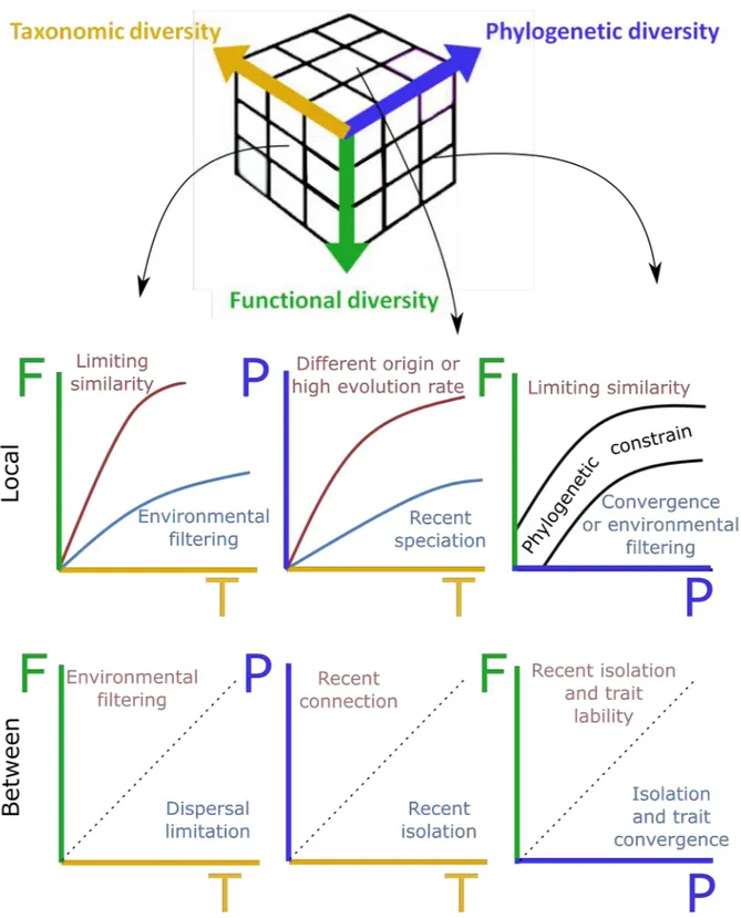
Figure I.6: Combining information on taxonomic, functional and phylogenetic diversity can help to
disentangle the main processes that structure communities, both within- and between-communities. On each plot, dominant processes are indicated. For local processes (α-diversity), the main expectation is that higher taxonomic diversity causes higher functional and phylogenetic diversity. Deviation from this expectation (blue and red lines) indicates that one process structure local community. Phylogenetic and functional diversity must be correlated (phylogenetic constrain or trait conservatism), but communities can deviate from it. For between-communities diversity (β-diversity), the more dissimilar the communities are in their species identity, the more functionally and phylogenetically dissimilar communities will be. Departure from this expectation indicates that one process is stronger than the other. Although each plot links only two facets, conclusions must be taken from the comparison of the three facets simultaneously
phylogenetic richness (Xiang et al., 2004).
On the other hand, if limiting similarity rules community assembly, each species will be ecologically different to the others (as a result of competitive exclusion), and hence will greatly contribute to increasing functional richness, more than under a random species selection (Mouillot et al., 2007). If species present in the community originate from different regions (following recolonization or after introduction) or if evolutionary or speciation rates are faster due to particular environmental conditions (barriers to gene flows, habitat heterogeneity) or biological attributes of species (dispersal rates, population structure), phylogenetic richness will greatly increase (Xiang et al., 2004).
Lastly, the relationship between functional and phylogenetic α-diversity, if deviating from the expectation that more distant species are more functionally different, can either reveals limiting similarity (if close related species occurrence causes higher functional richness than expected) or indicates dominant and strong environmental filtering that causes strong niche conservatism or trait convergence, with distant species having similar ecological traits (Safi et al., 2011).
β-diversity relationships
For β-diversities relationships, the main expectation is that the more pairs of communities will have different species (higher β-diversity), the more they will be different both functionally and phylogenetically, due to increasing environmental differences and isolation by distance. Deviation from this null expectation, with one diversity facet being higher or lower than the other, can inform which processes dominate community structure.
If communities are composed of different species (high taxonomic β-diversity) but these species are ecologically similar (low functional β-diversity), this could provide hints for strong dispersal limitation between communities, preventing species to occur in both communities (Fukami et al., 2005). This dispersal limitation can be caused by the presence of a barrier to the dispersion or can result from different colonization history and competitive exclusion (Fukami, 2015). On the opposite, communities with similar species composition but with some species that differ greatly in their ecological attributes can result from differences in particular environmental conditions between the two sites that select for species with specialized ecology.
Comparing taxonomic and phylogenetic β-diversities can help to differentiate between dispersal limitation caused by recent or ancient isolation (Weinstein et al., 2014). Ancient isolations of communities result in independent evolution of communities that causes high values of dissimilarities in both diversities. If communities were recently isolated, they had the possibility to exchange species before isolation and species of the communities will be phylogenetically related. After the isolation, communities evolved independently, but not during a sufficient time to blur their past common history, thus resulting in lower phylogenetic dissimilarities than expected. On the opposite, recent connection between previously isolated assemblages can allow the exchange of some phylogenetically distant species
Introduction
between communities (the one that can colonize new communities), thus reducing taxonomic dissimilarity between communities. However phylogenetic dissimilarity will stay relatively high compared to taxonomic dissimilarity.
Lastly deviations from the expected relationship between functional and phylogenetic β-diversities can inform on traits convergence between isolated communities in similar environmental conditions or high trait lability in recently isolated communities (Swenson et al., 2012b; Yang et al., 2015). This last relationship is difficult to test, as phylogenetic diversity and functional diversity are independantly computed and thus cannot be decoupled.
Here I described relationships between diversity facets two by two. However, they must all be considered altogether to have the full picture of the processes. For example, observing low dissimilarities in the 3 diversity facets will reflect communities in similar environment with no dispersal limitation, whereas high dissimilarities in taxonomic and functional diversity but lower phylogenetic dissimilarity reflects recent isolations of communities that evolve in different environments.
Freshwater fish as a model to study assembly rules
This framework thus needs exhaustive information on the communities and on the species that compose them. Rich and variable communities might be promising cases to disentangle assembly processes. Within Neotropical regions, plants communities and their assembly processes have been heavenly studied (Kraft et al., 2008; Swenson et al., 2012a; Kraft & Ackerly, 2010; Fortunel et al., 2014). In contrast, freshwater fish assemblages have long been restrained to species inventories, species-habitat relationships and anthropogenic impacts on the species. Building on those previous knowledge helps analysing assembly rules. Among freshwater organisms, fish are the best known, they benefit from a quite exhaustive taxonomic knowledge and from information (at least partial for tropical species) on species distribution. They therefore constitute an interesting biological model for studying assembly rules. Moreover, freshwatrer fises are ectothermic organisms and their distribution is thus highly constrained by their environment. Moreover, their movement depends on their own capacity, but also on the configuration of the hydrological network (Landeiro et al., 2011). This network also represents a closed environment for freshwater fishes, as the marine water represents barrier to their dispersal between the different drainage basins. The history of drainage basins will thus be reflected in the fish communities (Hugueny, 1989). All these characteristics thus affect how environment, space and past history structure fish assemblages and will modulate the strength of the assembly processes.
Within freshwater tropical fauna, fish from French Guiana benefited from extensive inventories in the seventies that led to the publication of the atlas of Freshwater fish from French Guiana (Planquette et al., 1996; Keith et al., 2000; Le Bail et al., 2000) and to gather solid information about the taxonomy of this speciose fauna. This knowledge on fish taxonomy and distribution constitute the first, but essential, step to unravel the
processes that structure fish assemblages.
I.2 Application to French Guiana freshwater fish assemblages
I.2.1
The Guianese territory
French Guiana is a French overseas department and region located on the Northwest coast of South America between Brazil and Suriname. It covers about 83,500 km2. Its coastal location close to the equator allows a relative homogeneity of the climate, with constant temperature around 25◦C. Only the rainfall highly varies between months
and determines two main seasons in French Guiana: the main dry season with low precipitation between September and December and two wet seasons (January to February and April to August).
The hydrological network is structured in 8 major drainage basins and small coastal creeks, that flow from South to North. The two largest drainages are the Maroni (65,830 km2) that form the Western boundary with Suriname and the Oyapock (26820 km2) at
the boundary with Brazil. The network represents 112,000 km of watercourse, with 80% being small streams of less than 1 m depth and 10 m wide. The downstream part of the network is under marine influence, with tide influence reaching up to 50 km long watercourse due to the low slope of the downstream part of the watersheds (Tito de Morais & Lauzanne, 1994).
I.2.2
Guianese demography and anthropogenic activities
Population in French Guiana have greatly increased since the late 1980 (Figure I.7), and is actually 4 times higher than in 1970. Until 1990, this increase was essentially caused by a high immigration rate that has reduced through the years. Even if the population growth rate slows down (+3.6% per year between 1999 and 2009, and +2.4% per year between 2009 and 2014; INSEE 2017), demographic models predict that population will exceed 300,000 inhabitants in 2030. The population is mainly concentrated on the coast, with 80% of the population located on a 20 km East-West coastal band.
This coastal band thus concentrates the majority of anthropogenic infrastructures (roads and urban area) and gathers the majority of industrial and agricultural activities that will mainly impact the downstream part of the hydrological network. On the contrary, the interior of the department is composed mainly of forest. Two main activities are conducted in the forested part of the territory: forestry and gold-mining. The forestry activity is managed by the National Forests Office (ONF) that sets rules to reduce environmental impacts of this exploitation on freshwater ecosystems. In addition, gold-mining activities are increasing (Hammond et al., 2007), especially localized non-legal mining that strongly impact freshwater ecosystems.
Introduction
Figure I.7: Evolution of Guianese population from 1954 to 2014 (—) and projection to 2030 from the
Omphale model (– – –). Data from INSEE (03/09/2017)
I.2.3
History and biogeography
French Guiana is part of the Guiana Shield, an upland region of South America, which formed during Precambrian around 1.7 Ma (Lujan & Armbruster, 2011). The recent ichtyofauna of French Guiana however results from more recent events of sea level oscillations caused by the alternation of hot and cold periods, that occurred during Late Pleistocene (Boujard & Tito de Morais, 1992). During hot and humid periods, sea level raised and the huge quantity of freshwater discharged by the Amazon River created continuous littoral swamps that connected all the river mouth of French Guiana and homogenized the ichtyofauna between drainage basins. These swamps also contributed to the colonization of fish species from the Amazon River to the East and from the Essequibo River and Rio Branco Riverto to the North. During subsequent cold period (-18,000 years), sea level went down and the littoral swamp reduced. The connection between the different drainage basins stopped, except between a few neighboring basins (Maroni and Mana on the West and Approuague and Oyapock on the East). The isolation of some fish led to speciation cases, probably explaining the current differentiation between Western and Eastern basins (Le Bail et al., 2012; de M ´erona et al., 2012). In addition, river captures events in the upper portion of rivers had also favored species colonization of the headwaters from the South between Guianese and Amazonian tributaries (Cardoso & Montoya-Burgos, 2009). All these events thus contributed to the large diversity and organization of freshwater fish in French Guiana.
I.2.4
Aquatic ecology
Guianese freshwater fish fauna counts of 405 species, with 386 strictly freshwater fish species, from 12 orders (Siluriformes and Characiformes are the most represented). 26
91 of these species (26%) are endemic of drainage basins located in French Guiana. Within French Guiana, wider drainage basins have more fish species (de M ´erona et al., 2012), and species identity differs between Eastern and Western drainage due to past history of the region (Le Bail et al., 2012).
Ecological studies conducted on freshwater fish assemblages in French Guiana have been mainly conducted on the main rivers, especially on the Sinnamary and the Approuague Rivers leading to distinguish fish fauna from estuaries, middle and upper main streams and headwaters (Tito de Morais & Lauzanne, 1994; Boujard & Rojas-Beltran, 1988). At a lower scale, five types of habitats have been described (Boujard et al., 1990): creeks or small streams (width 10 m and depth 1 m), rapids (high flow and important presence of rocks) and pools with different bottom substrates (eroded concave part, sedimentary convex part and intermediary).
Freshwater stream assemblages and anthropogenic disturbances
Studies of stream assemblages started in the 90ies with extensive studies on the streams of the Sinnamary basin before and after the filing of the Petit-Saut‘s dam, an hydroelectric barrage on the middle course of the Sinnamary River, focused the attention of freshwater ecological studies toward this river and its tributaries. Those studies led to analyses fish densities according to habitat structural complexity, with higher density in habitat with higher complexity, water level and distance of the site to the river (M ´erigoux & Ponton, 1999). Spatial variation in assemblages was linked with water quality (oxygen and turbidity) that affect the identity of species according to their life-history traits between streams.
More recently, the development of illegal mining activities led to extensive works on small forest streams with the aim to quantify the strength of the mining disturbance on aquatic assemblages (fish and benthic macroinvertebrates). This work conducted during Allard (2014) and Dedieu (2014) PhD theses, allowed to sample over 150 sites throughout Guiana, in both undisturbed and disturbed (gold mining and logging) environments. Physical and chemical characteristics of undisturbed and logged sites were similar, but logged sites had finer bottom particles (Dedieu et al., 2014). However, gold mined sites greatly differed from undisturbed sites, with higher water turbidity and coarser bottom particles, especially gravel. This modification of the local habitat translated in a modification of assemblage structure (Dedieu et al., 2015; Allard et al., 2016). Both taxonomic and functional structure of assemblage differed between undisturbed and gold mined sites, with a shift from small stream specialist species to larger ubiquitous species inhabiting rivers for fish and from herbivorous and swimmers species to endobenthic burrowers and collector filterers for macroinvertebrates (Figure I.8).
Although these works contributed to understand how tropical streams and freshwater assemblages are affected by anthropogenic disturbances, the processes that structure local assemblages remained poorly known.
Introduction
Figure I.8: Modification of Guianese freshwater assemblages by anthropogenic disturbances.
Taxonomic structure of Ephemeroptera assemblages (a, distribution of genera; b, distribution of sites clustered by site condition based on taxonomic data) and functional structure of fish assemblages (c, correlation circle of fish functional traits; d, positioning of each site condition centroids based on functional data) differed between undisturbed and logged sites, and gold-mined sites. Abbreviations used in c: Phyto: phytophagous species; SL max: maximum standard length; Ubiquit: ubiquitous species; Omni: omnivorous species; Pred: predatory species. Figures from Dedieu et al. (2015) and Allard et al. (2016); Ephemeroptera image by George Starr (CC BY-NC-SA 3.0)
I.3 Thesis
I.3.1
Aim
Previous work on freshwater fish of French Guiana highlighted the impact of anthropogenic disturbances on these assemblages, both in large rivers and small streams. Understanding the processes that govern these assemblages will help evaluating future impacts of anthropogenic disturbances. The main goal of my thesis was thus to elucidate the assembly rules that govern freshwater fish assemblages of French Guiana. To do, I combined information on 4 types of data: taxonomic, functional and molecular data, and site descriptors.
I.3.2
Taxonomic data: assemblage composition in streams and
rivers
Stream fish assemblage composition was obtained from sampling during the dry seasons, with a single sampling occasion by site (except for a few sites). Fish were collected using rotenone, a non selective piscicide. Rotenone is a chemical compound from the ketone family, naturally produced by tropical plants of the Leguminosae 28
family found in Australia, Southeast Asia and South America, like jewel vines Derris spp. or lacepods Lonchocarpus spp. It acts by inhibiting cellular use of oxygen by gill-breathing organisms (Lindahl & ¨Oberg, 1961). This aspect implies that it also affect not only fish, but also freshwater insects, and have thus a strong disturbing effect on local fauna. Nevertheless, it is the only method available to get a good picture of local fish assemblages (Allard et al., 2014). To limit its impact, sampled sites were located closed to a confluence to dilute Rotenone and weaken its effect downstream. Moreover, the lowest possible quantity of rotenone was used, and downstream fish mortality was never observed. All the samples were authorized by the French ministry of environment (DEAL), and the Guianese National Park (PAG) when samples were taken in streams belonging to the PAG.
The sampling protocol takes place as follows: i) a portion of the stream is isolated with fine mesh (4 mm mesh size) stop nets to avoid fish escape out of the station (Figure I.9a); ii) the rotenone is introduced upstream and homogenized before and in the portion; iii) fish are collected; iv) when all fish have been collected, a last passage is made to collect fish lying at the bottom of the stream; v) nets are removed and fish stopped by them collected; vi) fish are identified directly or stored to be identified later. The portion of the stream isolated was defined to represent one hydromorphological unit (pool, riffle, rapid, fall or run), but was sometimes constrained by the presence of obstacles in the stream, (e.g. trees and branches fallen in the stream making areas where collecting fish is not possible). Several subsequent portions were sampled on the same stream in some sites to represent the hydromorphological diversity of the stream.
Most of the samples were collected during Allard (2014) thesis, as part of a Guiana National Park-DEAL-HYDRECO project (2011-2014), but some sites have been sampled under other projects: CNRS-Nouragues projects (2008; 2010), PAG Itoupe project (2010), DIADEMA project (LabEx CEBA, 2013-2015), and Our Planet Reviewed Mitaraka project (2015).
For rivers, fish are collected using 50 meters long gill-nets with different mesh sizes (from 15 to 35 mm). In each site an overnight sampling with a standard set of 20 gillnets was achieved. Gill-nets are placed on riverbanks (Figure I.9b). The nets are taken out of the water the following morning and identified after all nets removal. Contrary to streams, each site was sampled several times among the years. These samples are conducted to comply with the European Water Framework Directive (DCE). Fish surveys are part of DEAL and OEG projects, and technically operated by Hydreco lab, with the contribution of the EDB lab members (S. Brosse and myself) in Maroni and Approuague sites.
For my thesis, I used sampling data ranging from 2007 to 2016. Although abundance data can help to disentangle some of the assembly processes (e.g. competition between species), the differences in sampling protocol and in sensibility of species to each sampling methods can bias conclusions on assemblages determinants. We thus chose to convert all abundance data into occurrence data.
Introduction
Figure I.9: Examples of stream (a) and river (b) sampling sites. (Photo: L. Allard and I. Cantera)
I.3.3
Functional data: morphological measures and functional
traits
To compute functional diversity of assemblages, we used 15 functional traits that account for two main functions: locomotion and nutrition. These functional traits have been widely used to asses functional diversity of fish assemblages (Vill ´eger et al., 2017; Leit ˜ao et al., 2017). The lack of ecological knowledge on Guianese fishes prevented from estimating others key functions (life history strategy, feeding composition). For each species, I extracted 14 morphological measures from Toussaint et al. (2016) database that contain morphological measures. In addition, we took pictures of fish during 2015 and 2016 sampling sessions to complement our functional database (32 species) and to maximize the number of individuals per species, to reduce potential bias due to intraspecific variability.
The morphological measures are taken from photographs on a lateral view of the fish (Figure I.10 and Table I.1a) and characterize body shape and fin size and surface, eye and mouth size and position. In addition to these measures, the maximum length of each species was recovered from Froese & Pauly (2015).
Figure I.10: The 14 morphological measurements taken on each fish species to calculate the functional
traits
These measures were then combined into ratios that described body shape, fins eye and mouth relative position on the body or their relative size. These ratios reflect species capacity to feed (prey capture and detection, location in the water column) and to swim (Table I.1b, Vill ´eger et al., 2017; Toussaint et al., 2016).
Table I.1: The 14 morphological measurements used (a) and the functional traits calculated (b) on each
fish species
(a) Morphological measurements
Symbole Name Definition
Bl Body length Standard Length
Hd Head depth Head depth along the vertical axis of the eye
CPd Caudal
peduncle depth
Minimal caudal peduncle depth
CFd Caudal fin
depth
Maximum depth of caudal fin Ed Eye diameter Vertical diameter of the eye
Jl Maxillary Jaw
Length
Length from snout to the corner of the mouth
Bbl Barbel
maximum Length
Length of the longest barbel
PFl Pectoral fin
length
Length of the longest ray of the pectoral fin
PFi Pectoral fin
position
Vertical distance between the upper insertion of the pectoral fin to the bottom of the body
Bd Body depth Maximum body depth
Eh Eye position Vertical distance between the centre of the eye to the bottom of the body
Mo Oral gape
position
Vertical distance from the top of the mouth to the bottom of the body
CFs Caudal fin
surface
Total fin surface
PFs Pectoral fin
surface
Total fin surface MaxLength Maximum
length
Maximum adult length (obtained from FishBase (Froese & Pauly, 2015))
Introduction
Table I.1 continued
(b) Functional traits
Component Functional traits Measure Relevance
Maximum length Log(M axLength) Metabolism, trophic impacts, locomotion ability, nutrient cycling
Prey detection Eye size Ed
Hd Visual acuity (Boyle & Horn, 2006)
Barbel length BblBl Detection of hidden preys
Prey capture Oral gape position M oHd Feeding position in the water column (Dumay et al., 2004; Lefcheck et al., 2014)
Maxillary length J l
Hd Size and strength of jaw
Position in the water column
Eye position EhHd Position of fish and/or of its prey in the water column (Winemiller, 1991)
Body elongation BdBl Position of fish and/or of its prey in the water column(Winemiller, 1991)
Swimming Body lateral shape Hd
Bd Relative depth of the head compared to the body
Pectoral fin position P F iBd Pectoral fin use for maneuverability(Dumay et al., 2004) Pectoral fin shape P F l2
P F s Pectoral fin use for propulsion (Fulton et al., 2001)
Pectoral fin size P F l
Bl Pectoral fin use for propulsion (Fulton et al., 2001)
Caudal peduncle throttling
CF d
CP d Caudal propulsion efficiency through reduction of drag (Webb,
1984) Caudal fin aspect
ratio
CF d2
CF s Caudal fin use for propulsion and/or direction (Gatz, 1968;
Webb, 1984)
Fin surface ratio P F sCF s Fin use for swimming
Relative fin surface (P F s+CF s)(Bl×Bd) Fin total surface compared to body lateral surface
I.3.4
Molecular
data:
molecular
markers
and
phylogenetic
relationship
During field sampling campaigns and fish collection, a small piece of fin was collected on at least 3 individuals per species belonging to different drainage when possible. In total, 6896 individuals were sampled, belonging to 259 species. DNA from these tissue samples were extracted at EDB laboratory using salt-extraction protocol (Aljanabi & Martinez, 1997). Three mitochondrial markers were first amplified: the cytochrome c oxidase I gene (COI), the cytochrome b gene (cytb) and the mitochondrial 12S ribosomal RNA (12S rRNA, or 12S). The cytb marker was removed from the analyses as amplification failed for a substantial part of the samples, and the remaining data did not provided additional information to COI and 12S data. I also included all the sequences available on GenBank, although Guianese freshwater fish are poorly informed in Genebank (142 species have at least one of the two makers). COI and 12S were used to reconstruct phylogenetic relationships between species. The 12S was also used to build the reference database for barcoding studies. After extraction, amplification and sequences cleaning, the molecular data contains 943 sequences. COI and 12S were informed for 422 individuals, COI only was informed for 386 individual, and 135 individuals were informed only for 12S.
I.3.5
Sites descriptors: environment and space
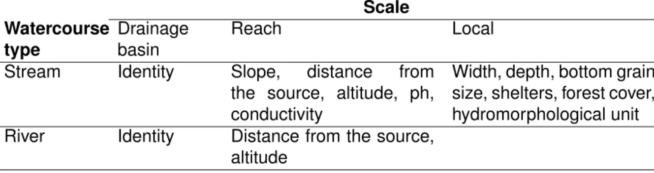
In addition to species related information, environmental characteristics of sites were obtained from field measurements and geographic information system (GIS). These descriptors can be categorized in 3 spatial scales: drainage basin, stream or river reach and local environmental features (Table I.2).
At the drainage basin scale, the identity of the drainage basin in which the site is located was used to distinguish between basins.
At the reach scale, distance from the source, slope and altitude were obtained from GIS and represent the position of the site in the upstream-downstream gradient of the hydrological network. For streams, the pH and the conductivity of the water were also considered as reach descriptors. They were measured on the field with a pH meter (WTW pH 3110 with WTW pH-SenTix 41 electrod) and a conductometer (WTW Cond 3310 with tetraCon 325 captor).
At the local scale, each stream portion was described by its hydromorphological unit (pool, riffle, run, according to the typology of Malavoi & Souchon, 2002), , the forest cover, its bottom grain size (silt, sand, gravel, pebble, boulder and bedrock), the presence of shelters for fish (wood, macrophytes, litter, under-bank and tree roots) and its width and depth. For width, at least 3 measures were taken perpendicular to stream flow, and along each line, the stream depth was measured every metre.
In rivers, local variables were not measured, because fish sampling is achieved using a net sampling with 20 50-metres long gillnets (15 to 35 mm mesh sizes). Sampling therefore occurs over the entire reach, encompassing heterogeneous local
Introduction
features.
Table I.2: Variables used to describe streams and rivers can be classified into 3 classes of spatial scale:
drainage basin, reach and local scales.
Scale Watercourse type Drainage basin Reach Local
Stream Identity Slope, distance from
the source, altitude, ph, conductivity
Width, depth, bottom grain size, shelters, forest cover, hydromorphological unit
River Identity Distance from the source,
altitude
I.3.6
Thesis conduct and structure
The above described data was used to investigate assembly rules of Guianese freshwater fish following these three main points:
1) Description of the diversity of streams fish assemblages: I first described spatial patterns of fish taxonomic diversity in streams, and investigated the environmental determinants of species richness and composition in these streams. I also investigated how space and environment shape the change in species composition between assemblages (manuscript A).
2) Assembly rules of freshwater assemblages: In this chapter, I elucidated the processes that structure freshwater fish assemblages, both in streams and in rivers, using all the information available on assemblages (taxonomic, phylogenetic and functional data). In a first part, I compared temperate and tropical stream assemblages (manuscript B), that are known to differ in their α-diversity and β-diversity. Using taxonomic and functional diversities, I tested if these differences could be explained by different strength in the processes that structure assemblages. Then I focused on Guianese assemblages and used the multi-faceted approach, with the taxonomic, functional and phylogenetic data to elucidate these processes.
3) A new sampling protocol: Stream assemblage data were obtained using rotenone, a toxicant that kills local fauna, which use is now banned by the law. River assemblage data, collected using nets placed on riverbanks, only represent a small fraction of the fauna and cause substantial fish mortality. Developing a new sampling protocol that can be used in both streams and rivers and that provides an exhaustive image of assemblages is a crucial step to pursue ecological studies in French Guiana. I thus tested the efficiency of eDNA metabarcoding, a new and promising molecular sampling method, to detect fish species, recover assemblage composition and to describe ecological patterns (manuscript C).
For each part, a summary of the corresponding manuscript is given to introduce the chapter.
undisturbed small streams
II.1 Summary
Compared to the temperate freshwater ecosystems that set the basis for freshwater ecological concepts, tropical streams have received less attention, and studies and management of these streams are highly driven by the temperate concepts. This situation is even more pronounced for small tropical streams and the fish assemblages they host. Indeed tropical lowland streams have easier access for sampling and they host more species with economical interest that the small upstream watercourses. In French Guiana, the first ecological studies of freshwater fish assemblages have thus been devoted to large rivers (especially the Sinnamary and the Approuague Rivers). In contrast, fish assemblages of the small streams have been mainly studied through the effect of anthropogenic disturbances on fish assemblage composition (Allard et al., 2016). Without information on the structure of freshwater fish assemblages and its determinants, predictions of fish assemblage and evaluating the impact of anthropogenic disturbances on them remain limited.
We used fish assemblage structure and environmental descriptors for 152 undisturbed sampling sites to describe the patterns of diversity in these streams (species richness and assemblage variation). We then evaluated the effect of environment and space (distance between sites) on these patterns. Each site was described at three spatial scales: the drainage basin scale (corresponding to the identity of basin), the reach scale (position in the upstream-downstream gradient and physic-chemical characteristic) and the site scale (forest cover, shelters presence, bottom grain size, width and depth). For the site scale, we used two different approaches to analyze species richness and assemblage variation: for species richness analyses, we calculated a habitat diversity index using the different categories of shelters and grain size, and classes of width and depth, whereas for assemblage variation, we kept separate these variables. This choice was guided by the niche theory that stipulates that the number of species in a site is related to the habitat diversity, whereas the identity of species is related to the habitat characteristics. In addition to these site-specific descriptors, we also took into account spatial relationships between the sites, based on the distance along the stream between sites located within a same drainage basin.
Species richness in the sites increased from upstream to downstream and in sites with higher habitat diversity. These patterns also hold for in the main fish orders (Characiformes and Siluriformes), testifying that the global pattern did not result from the replacement of different groups of fish. This upstream-downstream gradient was however marked by a succession of five group of species that characterize five main types of stream habitats (Figure II.1): altitude and torrential streams (1), small (2) and large (3) non-torrential streams , muddy streams (4) and confluence areas with larger
Chapter II: Diversity in streams
Figure II.1: Small streams of French Guiana can be divided into five main types areas along the
upstream to downstream gradient. Main characteristics of the area are indicated on the left and some characteristic species of the area on the right. (Photo: L. Allard, S. Brosse, I. Cantera, K. Cilleros, F. Melki, Guyane Wild Fish, M.N.H.N.)