HAL Id: hal-00329268
https://hal.archives-ouvertes.fr/hal-00329268
Submitted on 1 Jan 2003
HAL is a multi-disciplinary open access
archive for the deposit and dissemination of
sci-entific research documents, whether they are
pub-lished or not. The documents may come from
teaching and research institutions in France or
abroad, or from public or private research centers.
L’archive ouverte pluridisciplinaire HAL, est
destinée au dépôt et à la diffusion de documents
scientifiques de niveau recherche, publiés ou non,
émanant des établissements d’enseignement et de
recherche français ou étrangers, des laboratoires
publics ou privés.
High-latitude dayside ionosphere response to Pc5 field
line resonance
F. Pitout, P. Eglitis, P.-L. Blelly
To cite this version:
F. Pitout, P. Eglitis, P.-L. Blelly. High-latitude dayside ionosphere response to Pc5 field line resonance.
Annales Geophysicae, European Geosciences Union, 2003, 21 (7), pp.1509-1520. �hal-00329268�
High-latitude dayside ionosphere response to Pc5 field line
resonance
F. Pitout1, P. Eglitis2, and P.-L. Blelly3
1European Space Agency, Noordwijk, The Netherlands 2Swedish Institute of Space Physics, Uppsala, Sweden 3Centre d’Etude Spatiale des Rayonnements, Toulouse, France
Received: 13 May 2002 – Revised: 15 November 2002 – Accepted: 19 November 2002
Abstract. We report observations of pulsations due to Field Line Resonance (FLR) in the morning sector of the high-latitude dayside ionosphere on 1 February 1998. The Geo-tail spacecraft, ideally skimming the dayside magnetopause, monitored the magnetopause motion, which is seen to induce a modulated response of the ionosphere by means of ULF waves. Pulsations in the Pc5 frequency range were observed in the ground magnetic field measured by the IMAGE ar-ray, as well as in the electron and ion temperatures measured by the EISCAT Svalbard Radar. The ion temperature oscilla-tions are an indicator of a modulated convection electric field while field-aligned currents (FAC) associated with the FLR control the electron temperature. We have performed a sim-ulation of the ionosphere experiencing sinusoidal FAC and electric field in order to confirm our hypothesis. In addition to the ionospheric response, the possible cause of the FLR and processes involved are also discussed.
Key words. Magnetospheric physics (MHD waves and in-stabilities; magnetosphere-ionosphere interactions) – Iono-sphere (polar ionoIono-sphere)
1 Introduction
The magnetohydrodynamic theory of resonance (South-wood, 1974; Chen and Hasegawa, 1974a, b) explains ba-sically that magnetopause motion of any kind (global mo-tion, surface waves, Kelvin-Helmoltz instabilities) leads to the generation of compressional fast-mode waves that prop-agate in the magnetosphere across the magnetic field. At the so-called resonance region, the compressional mode converts into shear Alfv´en mode that propagates along the Earth’s magnetic field lines and carries energy down to the iono-sphere (field-aligned currents). Also, further in the flanks, magnetosheath plasma flow along the magnetopause may lead to a velocity shear, source of Kelvin-Helmoltz instabili-ties (KHI). The resulting surface waves propagate in an
anti-Correspondence to: F. Pitout (fpitout@rssd.esa.int)
sunward direction along the magnetospheric flanks. The en-ergy from the KHI is able to penetrate and propagate into the magnetosphere as compressional and shear-Alfv´en waves, as explained above.
However, it seems that the trigger processes are slightly different depending on which flank of the magnetosphere is considered. It is believed that FLRs in the dawn side are most of the time due to the over reflection process (Mann et al., 1999), whereas on the dusk side FLRs tend to be driven by solar wind buffeting or running pulse propagating along the magnetopause. This may be explained by the fact that interplanetary magnetic field lines hit the magnetopause tan-gentially on the dusk (garden hose effect). Therefore, the magnetic stress may act to stabilise the dusk magnetopause. Moreover, field line resonances in the morning and after-noon sector seem to have different properties (Ziesolleck et al., 1994).
Geomagnetic pulsations in the Pc5 range (period 150– 600 s) due to FLR have already been studied with numer-ous instruments. The most obvinumer-ous and best-known effect of ULF waves can be seen in ground magnetic field data (e.g. Mathie et al., 1999). Many observations report about the typical Pc5 frequencies that are naturally excited: around 0.9, 1.3, 1.9, 2.7 and 3.3 mHz. It has been shown that these frequencies correspond to waveguide modes in the magneto-sphere (Samson et al., 1992). Other frequencies have nev-ertheless been observed. Earlier studies proposed that those frequencies could actually be waveguide mode frequencies somewhat shifted due to various reasons. On the other hand, Ziesolleck et al. (1995) showed that the cavity/waveguide mode frequencies do not necessarily represent a unique set of frequencies.
FLRs have also been studied with ionospheric radars. Co-herent scatter radars were used (Ruohoniemi at al., 1991) in order to study the plasma convection during intervals of Pc5 pulsations. In some cases, similar typical frequencies were found in the plasma velocity oscillations associated with FLR. It has been reported, however, that in some other cases, there was a disagreement between radar and magnetometer
1510 F. Pitout et al.: Polar ionosphere response to FLR
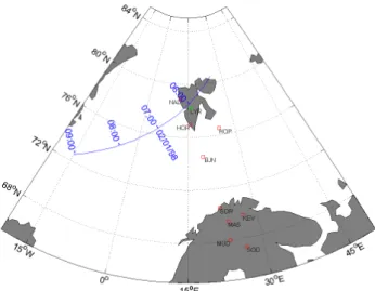
Fig. 1. Observational configuration of 1 February 1998 showing Geotail projected orbit in the Northern Hemisphere’s ionosphere (in blue), the EISCAT Svalbard Radar and the neighbouring IM-AGE station in Longyearbyen (in green) and the nine other IMIM-AGE stations (in red).
measurements of the same Pc5 field line resonances. This is partly due to the different fields-of-view of the instruments (Ziesolleck et al., 1998). A magnetometer measurement is typically derived from integration over an area of 100 km2in
the lower ionosphere; radar measurements have finer spatial resolution.
Most of the studies dedicated to ULF Pc5 oscillations were performed with magnetometers and/or HF radars. Studies of the response of the ionospheric plasma to ULF waves are more rare. Yet, even incoherent scatter radars point to field-aligned record features in the ionospheric plasma related to ULF waves (Lester et al., 2000; Buchert et al., 1999). It was reported in those two papers that ULF waves are accompa-nied by pulsed high-energy electron precipitation. We also expect some ion heating associated with ULF waves, as dis-cussed by Lathuill`ere et al. (1986).
At last, some articles have been published very recently attempting to explain and/or separate the different processes which are believed to be responsible for FLRs. For example, Mann et al. (1999) consider three basic processes that they distinguish by azimuthal phase speed considerations: impul-sive buffeting (IB), running pulse (RP) and over-reflection (OR).
Our objective is to study and understand the ionospheric reaction to FLR at high latitude. While possible, we will test and discuss the different models in the literature. We add in this work the extra contribution of the ESR incoherent scatter radar located at high latitude. We will complete the interpre-tation of the ESR observations with numerical simulations performed using the ionospheric model TRANSCAR (Blelly et al., 1995).
Fig. 2. Solar wind parameters and interplanetary magnetic field measured at IMP-8.
2 Observations
The FLRs reported here were observed on 1 February 1998 in Northern Scandinavia, which is a rich region of ground-based instruments, with much overlap in each instrument’s field-of-view. Ten IMAGE ground magnetometers, the EIS-CAT Svalbard radar and an overpass of the Geotail spacecraft have been utilized (Fig. 1).
2.1 Solar wind and IMF: IMP-8
In order to have the external conditions in the solar wind and thus, the global context of our event, we have looked at data from the IMP-8 spacecraft. In a GSM system its coordinates are XGSM = 24 RE, YGSM = 5 − 10 RE, ZGSM =19 RE.
On board, the MAG instrument provides us with magnetic field measurements and the PLA instrument with plasma pa-rameters (density and velocity). Figure 2 displays IMP-8 data with, from top to bottom, the solar wind dynamic pres-sure, number density, velocity, as well as the three compo-nents of the IMF, Bx, By and Bz in GSM. The time delay
between IMP-8 measurements and the ground (magnetome-ter measurements) has been estimated to be 8 min. IMP-8 does not measure dramatic variations either on the dynamic pressure, or on the magnetic field throughout the period of
Fig. 3. Geotail data showing multiple magnetopause cross-ings/incursions. From top to bottom: ion density, ion velocity, and magnetic field amplitude.
interest (06:00–07:00 UT). The dynamic pressure remains fairly stable between 4 and 5 nPa. Nevertheless, there are variations and a close analysis will be performed in order to find out whether or not there are characteristic frequencies in those variations despite their weak amplitudes. It is im-portant to note that the IMF points northward throughout the whole time interval (except a very short southward incursion at about 08:50 UT).
2.2 Magnetopause: Geotail
One of the key instruments of this study is the Geotail space-craft. On 1 February 1998, it was skimming the subsolar magnetopause in the morning sector, near the GSM equa-torial plane (XGSM = +6 RE, YGSM = −10 RE, ZGSM =
+1 RE). Figure 1 shows the projected footprint of Geotail
orbit. Data from the LEP and MGF instruments are shown in Fig. 3, with, from top to bottom, the plasma density, the plasma velocity, and the magnetic field amplitude. Ini-tially, in the magnetosheath (high plasma density and veloc-ity, weak magnetic field), the spacecraft clearly does several incursions in the magnetopause/magnetosphere (low plasma density and velocity, strong magnetic field). The velocity shear between the magnetopause and the magnetosheath, as well as the magnetic field discontinuity is clearly present in
Fig. 4. X-component of the ground magnetic field between 06:00 and 07:15 UT recorded by 10 stations of the IMAGE array. For each station, its name sits on the left and its magnetic latitude (CGM) on the right.
the data. The sunward component of the flow velocity (X-component) varies between −350 km/s in the magnetosheath and is about 0 in the magnetosphere. The magnetic field has strong values of about 50 nT within the exterior magneto-sphere and one order of magnitude less in or near the magne-tosheath. At least two of the incursions exhibit a character-istic feature of magnetopause crossings: outbound crossings look turbulent in magnetic field data, whereas the inbound crossings look sharper (Kawano et al., 1994).
2.3 Ground magnetic field: IMAGE magnetometer array IMAGE is the Fenno-scandinavian network of magnetome-ter operated by the Finnish Meteorological Institute, which extends from Uppsala in mid-Sweden up to Ny ˚Alesund on Svalbard. It is used in order to classify the geomagnetic pulsations. Each magnetometer gives 10-s resolution mea-surements of the 3 Cartesian components X, Y , Z of the ground magnetic field, aligned along geographic north, ge-ographic east and radially downwards, respectively. The X-component of the ground magnetic field measured at 10 cho-sen stations (Fig. 1) is shown in Fig. 4, for the time interval 06:00–07:15 UT, which is the period of interest of our study. The stations above BJN (71.33◦of magnetic latitude) show dispersed variations of the X-component of the ground mag-netic field. The maximum amplitude of those variations is
1512 F. Pitout et al.: Polar ionosphere response to FLR
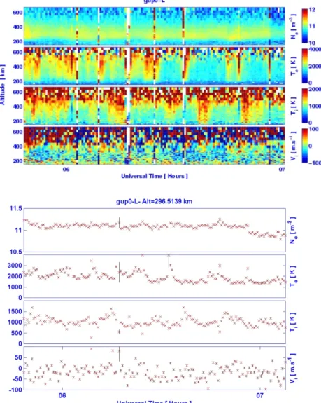
Fig. 5. Ionospheric plasma parame-ters measured by the ESR (dish point-ing field-aligned). Upper panel, from top to bottom: Ne, electron density, Te,
electron temperature, Ti, ion tempera-ture, and line-of-sight velocity, Vi
(pos-itive away from the radar) as a function of time and altitude. Lower panel: time series of the same parameters measured at 300 km of altitude.
about 80 nT. The stations below BJN recorded out of phase variations of smaller amplitudes. At lower latitudes, i.e. at auroral latitudes, the magnetic pulsations have much weaker amplitudes, typically a few tens of nT, with an irregular be-havior. No phase shift or dispersion is a priori noticeable among the low-latitude stations. A proper analysis of those pulsations is performed in Sect. 3.
2.4 Field-aligned sounding: EISCAT Svalbard Radar The ESR is the latest radar of the European Incoherent SCATter (EISCAT) scientific association. It is located on the Svalbard archipelago, near Longyearbyen (geographic coor-dinates 78.20◦N and 15.82◦E). The observations were per-formed field-aligned (azimuth 180.6◦, elevation 81.6◦). The region of resonance lies at ∼72◦MLAT; this is key region in which to study FLRs. However, it is important to make observations at neighbouring latitudes in order to diagnose the correct behaviour of the whole magnetosphere system. In this context, the contribution of the ESR is very impor-tant. We can observe FLRs south of the open/closed field
line boundary and look at the FLR signature in fundamental properties of the plasma (density, temperatures, velocity).
According to IMAGE data (Fig. 4) and more particularly, to the Longyearbyen (LYR) station, the ESR observes the northernmost resonant field lines. Considering the time of observation and the northward IMF, the ionosphere above the ESR is expected to be tenuous and cold. ESR data are shown in Fig. 5. The maximum density and temperature of the electron population in the F-region are 1011m−3and
2000 K, respectively. One can see, however, very faint and sporadic density enhancements corresponding to increases in the electron temperature, that suddenly go up to 3000 K. At this point, we may think about pulsed reconnection but we must remember that the IMF points northward throughout the whole period of interest. Consequently, the open/closed field line boundary must lie north of the radar. Moreover, the fact that the electron temperature increases without any significant electron density enhancement suggests that there is no or very little precipitation. Actually, it rather suggests that the heating of the electrons may be due at least partially
Fig. 6. Power spectra of various parameters. From top to bottom:
X-component of the ground magnetic field measured at LYR, idem at KEV, electron temperature measured at 300 km of altitude by the ESR, idem for ion temperature, magnitude of the magnetic field recorded at Geotail, and solar wind dynamic pressure recorded at IMP-8.
to field-aligned currents.
The ion population experiences the same quasi-periodic heating. As all the others plasma parameters, the typical val-ues of the ion temperature are low (1000 K or below) but at times, it peaks up to 2000 K. It is to be noted that ion tem-perature increases while electrons are cool. As it has been reported already by Lathuill`ere et al. (1986), the variation of the ion temperature observed in our case is undoubtedly due to oscillations in the convection electric field.
3 Data analysis
In order to examine and compare the data in a more rigor-ous way, we have performed a spectral analysis of the satel-lite data, magnetograms, and time series of the ionospheric plasma parameters measured by the ESR at a given altitude (300 km). Our analysis method consists first in filtering the data with a 0.5–5 mHz band-pass filter. The filter used is a 4th-order elliptic band-pass filter with 0.1 dB of ripple in the pass-band and 40 dB of attenuation in the stop-band. The choice of this frequency range is motivated by the fact that we expect the pulsations to belong to the Pc5 range of
fre-Fig. 7. Polarisation (negative values for clockwise polarisation; pos-itive for counterclockwise) and amplitudes X- and Y -components of the ground magnetic pulsations for three frequencies: 1.4 (plain), 1.8 (dotted), and 2.2 mHz (dash-dotted).
quency and by the results of previous studies showing that the wave-mode frequencies for FLR are typically several mHz. Then we classically Fourier transform the filtered signal and calculate the power spectrum of the signal. The data are anal-ysed over a one-hour period, fixing in theory the frequency resolution to ∼0.28 mHz. The time resolutions of the data set from the different instruments are 10 s for IMAGE and Geotail data, 30 s for ESR and 1 min for IMP-8. These time resolutions give Nyquist frequencies (twice the sampling fre-quency) used for signal processing of 200, 67, and 33 mHz, respectively.
Figure 6 shows the power spectra of, from top to bottom, the X-component of the ground magnetic field at Longyear-byen (LYR), at Kevo (KEV), the electron temperature as measured by the ESR, the ion temperature (a good indica-tor of the electric field) as measured by the ESR, the mag-netic field magnitude at the magnetopause/magnetosheath recorded at Geotail and the dynamic pressure in the solar wind recorded at IMP8.
1514 F. Pitout et al.: Polar ionosphere response to FLR
Fig. 8. Ionospheric plasma parame-ters modelled by TRANSCAR. Upper panel, from top to bottom: Ne,
elec-tron density, Te, electron temperature,
Ti, ion temperature, and line-of-sight
velocity, Vi (positive away from the radar) as a function of time and altitude. Lower panel: time series of the same parameters modelled at 300 km of alti-tude.
3.1 Pulsations in IMAGE data
Our choice for the IMAGE stations was driven by the lo-cation of the ESR radar at Longyearbyen (LYR) and the need for an auroral station (Kevo, KEV), located equator-ward from the disturbance. Note that spikes below 1 mHz should not be trusted, since we pass-band filtered the data be-tween 0.5 and 5 mHz. At Kevo, one can see four typical fre-quencies in the magnetic field, at 1.4, 1.8, 2.2 and 2.7 mHz. Those frequencies are very close to frequencies observed by Lessard et al. (1999). The authors observed field line reso-nance at 1.4, 1.7 and 2.1 mHz. It is the 2.7 mHz frequency which dominates the magnetic field at this latitude. Curi-ously enough, further north at LYR, the same 2.7 mHz fre-quency is absent. There, the magnetic field is dominated by the 1.4 mHz frequency. The two other frequencies at 1.8 and 2.2 mHz are also present, but their contributions to the signal are much weaker.
In order to highlight the properties of the observed
pul-sations and to find out where the resonance region is, we have displayed in the upper panel of Fig. 7 the polarization of the pulsations calculated at the same 10 stations for the three frequencies present at LYR (1.4, 1.8, and 2.2 mHz). Negative/positive values correspond, respectively, to clock-wise/counterclockwise polarization. We observe a character-istic feature of the resonance for the three frequencies: in the morning sector, the polarization changes from clockwise at low latitude to counterclockwise at higher latitude (Mathie et al., 1999). Also, the amplitudes of the X- and Y - components of the ground magnetic field shown in the second and third panels of Fig. 7 are maximal at the resonance.
From the first panel of Fig. 7, it is difficult to determine the exact latitudes of resonance, since those regions lie at high latitude in an area where the magnetometer coverage is not the most favorable (between mainland and Svalbard archipelago). This happens to be very likely due to the north-ward IMF that contracted the polar cap. However, according to the second and third panels in Fig. 7, the resonance regions
3.2 Pulsations in ESR data
The electron temperature at 300 km of altitude shows clearly two frequencies at 1.4 and close to 2.2 mHz. A third fre-quency is also present at 1.8 mHz, but this one appears much weaker in the power spectrum. As already evoked, this is a strong indication that the electron heating in the ionosphere is closely related to the wave activity and very likely due to the associated field-aligned currents.
The ion temperature also exhibits the same two typical fre-quencies at 1.4 and 2.2 mHz, although ion and electron heat-ing events do not occur simultaneously. This clearly indi-cates that the convection electric field is modulated by ULF waves. This has already been observed at lower latitudes (Lathuill`ere et al., 1986). On the other hand, the ion tem-perature pulsation does not contain the 1.8 mHz frequency observed weakly in the electron temperature. The phase shift between the electron heating (very likely due to a field-aligned current) and ion heating (due to frictional heating) implies a phase shift between the current Jkand the
perpen-dicular electric field E⊥.
3.3 Magnetopause motion
The fifth panel in Fig. 6 shows the power spectrum of the magnetic field as recorded by Geotail. A quick look at Fig. 6 reveals a close correlation between the typical frequencies of the magnetopause oscillations and those of the ionospheric parameters. We have found at least two waveguide modes being excited at 1.4 and 2.2 mHz. These frequencies ap-pear in the spectral analysis of all the parameters consid-ered: ground magnetic field, pressure recorded by Geotail,
Te measured by the ESR. This strongly supports the idea
that the magnetopause motion triggers the whole magneto-sphere/ionosphere pulsations.
3.4 Variations in the solar wind
The last panel in Fig. 6 displays the power spectrum of the solar wind dynamic pressure recorded at IMP-8. Although there are typical frequencies in the signal at 1.5, 1.9, 2.1 and 2.5 mHz and although some of them are interestingly close to those observed on the ground, it has to be noted that the corresponding powers are quite weak. The peak at 1 mHz is just at the filter edge and should, therefore, be ignored.
4 Simulation
We try here to reproduce and understand the high-latitude ionosphere response to Field Line Resonance (FLR) as ob-served by high-latitude incoherent scatter radars at the
EIS-species along a magnetic field line, which can possibly move horizontally with the convection. The outputs of this model are totally compatible with the parameters measured by in-coherent scatter radars and then we can compare the results of our modelling to the observations.
TRANSCAR does not automatically take into account couplings with the magnetosphere, though it is able to ac-count for the electrodynamic couplings. Besides the knowl-edge of the neutral atmosphere, which can be adjusted from the MSIS-90 empirical model by calibrating the model on a calm period (Blelly et al., 1996), it requires a minimum of inputs concerning the precipitating particles and the con-vection electric field. The precipitation can be given by for-tunate low-altitude satellite passes, while information about the convection can be inferred from observations.
The user also has the option to add field-aligned currents. Since we suggested in the previous sections that the electron temperature fluctuations were very likely due to field-aligned current, we have used this option to model the effect of FLR on the electron temperature. The input field-aligned current is given by: Jk(t ) = J1sin ω1t + Jssin ω2t with ω1 and
ω2the angular frequencies of the wave. We have obviously
taken the two main frequencies found in the plasma param-eters: 1.4 and 2.2 mHz (in the range of Pc5 pulsation). J1
and J2 have been chosen so that they take into account the
respective contributions of the two components to the total current (Fig. 9, third panel) and so that |Jk(t )| ≤2µA/m2.
Likewise, the electric field was calculated so that the fol-lowing condition between the perpendicular electric field of an Alfv´en wave and the field-aligned current the wave carries is fulfilled (e.g. Hasegawa and Uberoi, 1982), that is: Jk∝
∂E⊥ ∂t .
Therefore, the expression of the electric field is given by:
Ek(t ) = −E1cos ω1t − E2cos ω2t, and it is phase shifted by
90◦compared to the field-aligned current.
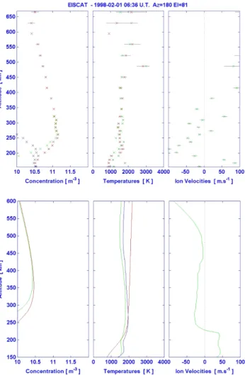
The result, partly shown in Fig. 6, reproduces what we could expect and what is observed, i.e. the electron density is not very affected, whereas the electron temperature shows the same periodic enhancements (corresponding to upward FAC) and decreases (corresponding to downward FAC) in the electron temperature. Due to the phase shift between the field-aligned current and the electric field, the ion tempera-ture goes up when the electrons are cool, as it is observed. More interestingly, the temperature profiles that we obtain from our modelling within electron or ion heating events are quite similar to those observed. Figures 9 and 10 show in the upper panels, from left to right, the measured altitude pro-files of the densities (electrons in red), temperatures (ions in green, electrons in red) and ion velocity along the line-of-sight. The lower panels display the same parameters (in the
1516 F. Pitout et al.: Polar ionosphere response to FLR
Fig. 9. Measured (top panels) and modelled (bottom) altitude pro-files of the plasma parameters within an electron-heating event (electrons in red, H+in green, molecular ions in blue).
same order), as modelled by TRANSCAR. The modelling of the densities is not relevant in our case, since we have not applied any background precipitation or any convection (transport effects not taken into account). Only the Sun’s in-sulation and the field-aligned currents are applied.
5 Interpretation and discussion
Here, we discuss the observed typical frequencies, the origin of the trigger of the ULF waves, as well as the response of the ionospheric plasma.
5.1 Pc5 field line resonance frequencies
The spectral analysis reveals characteristic frequencies. They are similar to those measured at Geotail and on the ground. This suggests that the magnetopause motion is the direct trigger of the whole magnetosphere-ionosphere oscillations. Even if the amplitude of the oscillations detected by ground magnetometers are weak (<100 nT), it is interesting to note
Fig. 10. Measured (top panels) and modelled (bottom) altitude pro-files of the plasma parameters within an ion-heating event (electrons in red, H+in green, molecular ions in blue).
how a moderate and stable solar wind leads to a clear re-sponse in the magnetosphere/ionosphere couple.
The latitudinal polarization profile along the chain of mag-netograms shows a change in polarization from counter-clockwise to counter-clockwise (from south to north) around BJN, logically corresponding to a maximum of the amplitude of the ground magnetic field. This indicates a resonance at those latitudes and presumably, some shear-Alfv´en waves travel-ling along the resonant field lines. A FAC should be carried by those waves.
These frequencies have to be compared with the expected frequencies from the waveguide model or observations (i.e. 1.3, 1.9, 2.6 mHz). At auroral latitude, KEV observes four main frequencies at 1.4, 1.8, 2.2 and 2.8 mHz. Why do we observe these frequencies and not exactly the one expected from the cavity mode models (Samson et al., 1992)? As men-tioned in the Introduction, it has been reported that magne-tometers give a slightly different result than HF radars, for instance, partly due to a different field-of-view. Except from the 2.2 mHz frequency, which is not predicted by the cavity mode model, the others are remarkably close to the stable
(IMAGE LYR, ESR and even Geotail). Actually, in our case, it is hard to believe that the frequencies found in the ground magnetic data are shifted, regardless of the reason. We find the very same frequencies in all the data. Previous work re-ported the occurrence of pulsations containing the 1.5 and 2.2 mHz frequencies (Ziesolleck et al., 1994) and were inter-preted in terms of fundamental, plus upper or lower sideband frequencies.
5.2 Physical process involved
We now investigate the cause of the FLRs. Surprisingly, the solar wind, which is thought to be a key parameter for driv-ing ULF waves, has a moderate velocity (=480 km/s) and its dynamic pressure is stable around 5 nPa. The IMF does not exhibit strong variations either. It has been suggested that Pc5 pulsations may be related to pulsed magnetic reconnec-tion at the dayside magnetopause (Prikryl et al., 1998). This is probably not the case here because the Z-component of the IMF is fairly positive all the time. The open/closed field line boundary lies in this case well north of the radar (Mc-Crea et al., 2000; Pitout et al., 2001). Besides, the density and temperature profiles measured by the ESR (Fig. 9) are totally different to those inside reconnected flux tubes (e.g. Lockwood et al., 2000).
Before using a more elaborate technique, we analyse the possible causes and see which can be eliminated:
1. The oscillations observed on the ground are rather irreg-ular and have weak amplitudes (∼80 nT at most). This tends to indicate that over-reflection (OR) does not take place and this process is not the cause of the waves we observe. OR usually leads to large amplitude waves. On the other hand, it is thought that a solar wind speed of at least 500 km/s is required to drive OR. Here, the veloc-ity recorded at IMP-8 is very close to that value (∼480 km/s).
2. Throughout the period of interest, the solar wind does not exhibit big changes either in speed, or in velocity direction, or even in magnetic field. Thus, it is hard to believe that a pulse running along the magnetopause could be responsible for our observations and this pos-sibility can be reasonably dismissed.
3. As already mentioned, the oscillations observed in the ground magnetic field are quite irregular and have small amplitudes, which fit the idea of a small amplitude and irregular motion of the magnetopause due to so-lar wind buffeting. Since Geotail was skimming the magnetopause, even very small amplitude variations of the solar wind pressure may make the magnetopause move slightly back and forth over the spacecraft. This
over-reflection, we use the diagnostic technique described by Mathie and Mann (2000) and Mann and Wright (1999). This technique is based on the analysis of the FLR azimuthal phase speed (APS). According to this diagnostic technique, if the APS for different modes calculated at the same local time between two different geographic locations on the ground (and thus, at the magnetopause) are different, the FLRs are due to impulsive buffeting of the magnetopause by the solar wind. If they are identical, one has to compare the APS with both the sound and Alfv´en velocities in the magnetosheath, in order to separate the over-reflection and the running pulse cases. The APS in the equatorial plane of the magnetopause is expressed as: Vph = 2π ReLf/m, where f is the
pulsa-tion frequency, Re is the radius of the Earth, L is the
McIl-wain parameter and m is the azimuthal wave number. The parameter m is the key parameter in this technique. We have used the KEV (magnetic coordinates 66.21◦N, 109.73◦E)
and the AND (66.36◦N, 100.92◦E) stations of the IMAGE
network in order to compare APSs. We have chosen two IMAGE stations, which have roughly the same magnetic lat-itude so that they belong to the same L-shell. By doing so, we avoid, or at least minimize, the latitudinal propagation ef-fects. Also, the fact that those two stations lie south of the resonance regions minimizes the phase changes associated with a resonance. In order to obtain the azimuthal wave num-ber m, we have simply calculated the phase shift between the waveforms (signal analysis described in Sect. 3) of the
Y-component of the ground magnetic field at those two sta-tions. The Y -component is less subject to phase changes due to resonance. The calculations lead to the same |m| (∼4) for three modes (1.5, 1.8 and 2.2 mHz) and thus, to differ-ent APS (∼180, 276 and 325 km/s, respectively, assuming
L∼12). The parameter m is in fact negative in our case, since the direction of propagation in the morning sector is westward (dawnward). The different values of APS tend to confirm that solar wind buffeting of the magnetopause trig-gers the FLR we observe.
5.3 High-latitude ionospheric plasma response
Before starting the discussion, it is important to note an inter-esting feature. The ionosphere is so cold that electrons and ions are at the same temperature within ion heating events (Fig. 10). This means that except for the wave activities, the ionosphere is very quiet and that there is no other processes involved that could possibly interfere and bring its own con-tribution in the radar data. There are basically four main rea-sons that make us think that the electron fluctuations seen in the ESR data are caused by field-aligned currents:
1. The electron density does not increase significantly when electron heating occurs.
1518 F. Pitout et al.: Polar ionosphere response to FLR 2. Between 06:00 and 06:45 UT, each electron-heating
event has at least one point (30 s time resolution) with-out data (Fig. 5, upper panel). There is actually data taken but the GUISDAP code that analyses the data as-sumes a Maxwellian distribution of particles and did not manage to fit the data to the model. It happens quite often that strong field-aligned currents lead to non-Maxwellian plasma and even to plasma instabilities, which therefore result in error in the analysis process. 3. The altitude profiles of electron temperature look very
similar to those expected in the presence of FACs. The temperature increases linearly with altitude until 200– 250 km and then increases very slowly (Fig. 9). 4. The phase shift between the electron and ion
tempera-ture strongly suggests a wave origin of what we observe, which implies a phase shift between the current and the perpendicular electric field associated with this wave. Those field-aligned currents are thought to be carried by shear-Alfv´en waves in the magnetosphere. They are indica-tive of the resonance process by which compressional fast mode waves convert themselves into shear-Alfv´en waves.
Unlike the observations reported by Buchert et al. (1999), we do not expect a significant modulation of the conductivi-ties in the F-region, since the electron density does not vary that much (for the reasons invoked above).
Nevertheless, is our case, it is hard to tell what the carriers are because we do not have access to the lower altitudes (E-region) and, therefore, to the high-energy particles.
One thing is sure; the electron density does not increase significantly in the F-region when the electron temperature increases. This means that the heating is not due to precip-itation, at least not directly. This does not mean that there is no precipitation, but that the precipitation does not ionise the medium in the F-region, rather very likely at lower al-titudes (high-energy precipitating particles on closed field lines). There are actually two other very effective heating processes in the upper F-region (above 300 km): the electron thermal conductivity and the thermoelectric effect (Blelly and Alcayd´e, 1994). In our simulations, the downgoing elec-tron heat flux at the upper limit of the model (3000 km) is needed in order to account for thermal coupling with the magnetosphere by thermal conduction. The heat flux qeand
the electron temperature Tesatisfy the classical Fourier’s law
approximation (Blelly and Alcayd´e, 1994):
qe= −αT
5/2
e ∂Te
dr ,
where α is the constant derived from the definition of the electron thermal conductivity K − e = αTe5/2(Banks et al.,
1976).
The heat flux at the topside ionosphere is assumed to be constant in time, so the former process can hardly be invoked to explain the temperature fluctuations. Besides, the electron temperature profiles would look very different. On the other hand, the thermoelectric effect due to a field-aligned current
has well-known effects on the ionospheric electron temper-ature (by modifying the total heat flux at a given altitude): downgoing (upgoing) FACs will increase (decrease) the total heat flux and, therefore, heat up (cool down) the electrons. In the presence of a FAC, the total heat flux can be expressed as: qe = −αTe5/2 ∂Te dr −β KBTe e J,
where β is a constant (Shunk, 1976), e is the electron charge,
kB is the Boltzmann’s constant, and J is the FAC intensity (Blelly and Alcayd´e, 1994).
There are some points that remain unclear though and they need to be clarified in the future. The variations in the solar wind, as well as those observed in the ground magnetic field, are rather weak and yet, the currents produced are rather high (2 µA/m2), in order to warm up the ionospheric electron pop-ulation. One can imagine a localised FAC that will dissipate easily in the ionosphere and, therefore, will be an effective source of heating (thermoelectric effect). However, the elec-tron heating is observed at ESR, i.e. slightly north of the resonance region. Does it mean that the FACs are not that localised? Does this imply a propagation process within the ionosphere?
6 Conclusion
We have reported observations of pulsations in the high-latitude ionosphere, and especially a response of the plasma parameters at ESR latitude (i.e. north of the resonance lati-tudes). The northward IMF made these observations possible by contracting the polar cap and bringing the resonance re-gion at or very close to ESR latitude. We have shown how the magnetopause motion is directly related to the wave ac-tivity in the magnetosphere and how the ionosphere reacts to these waves. The variations in the F-region electron tem-perature occur with the same fluctuation frequencies as the ground magnetic signatures. However, the electron density is not seen to follow the same trend.
Periodic enhancements of the electron temperature in the high-latitude dayside ionosphere are usually considered as the ionospheric signature of pulsed reconnection at the mag-netopause. Although Pc5 pulsation and pulsed reconnec-tion have been somewhat related to each other (Prikryl et al., 1998), in our case, it is clear that subsolar, pulsed re-connection cannot be invoked. We have showed in this study that Pc5 ULF waves also lead to periodic enhancement of the electron temperature in the dayside polar ionosphere.
The reason why electrons become heated in the F-region has been investigated. We have no convincing evidence of ionisation due to precipitating particles in the F-region, which makes us think that the source of heating is rather field-aligned currents. In addition, a preliminary TRAN-SCAR simulation of a quiet ionosphere experiencing a time dependant FAC of amplitude 2 µA/m2at most and contain-ing the two main observed frequencies gives a similar Te
Solar-wind/magnetosphere/ionosphere couplings by means of waves through magnetopause motion are indeed essential to understand the high-latitude dayside ionosphere, especially early in the morning and very likely late in the afternoon (in MLT). Until now, mainly the field response had been studied. We have shown that the ionospheric plasma reacts quite a lot as well. Unfortunately, the GUP0 modulation scheme does not allow us to probe altitudes lower than 170 km, approximately. We obviously do not have access to high-energy particle precipitation. Such observations have been reported using EISCAT facilities in Tromsø (Lester et al., 1999; Buchert et al., 1999). It would be very interesting to study the E-region’s reaction to ULF waves at high latitude as well. This should be possible with a more recent set of data using more recent modulation schemes.
Acknowledgement. The authors are grateful to the director and staff
of the EISCAT Scientific Association for providing the radar facil-ities and assistance with making the observations. EISCAT is an international association, supported the research councils of Fin-land, France, Germany, Japan, Norway, Sweden and the UK. We thank the institutes, which maintain the IMAGE magnetometers ar-ray. The IMAGE magnetometer data are collected as a Finnish-German-Norwegian-Polish-Russian-Swedish project. Geotail and IMP-8 orbit parameters were retrieved from SSC Web and IMP-8 data from CDAWeb. We thank R. Nakamura for providing us with Geotail data and for helpful comments. We are grateful to S. C. Buchert and F. Forme for fruitful discussions and for valuable com-ments on this manuscript. Topical Editor M. Lester thanks Y. Tonegawa and T. Yeoman for their help in evaluating this paper.
References
Banks, P. M., Shunk, R. W., and Raitt, W. J.: The topside iono-sphere: A region of dynamic transition, Ann. Rev. Earth Planet. Sci., 4, 381–440, 1976.
Blelly, P.-L. and Alcayd´e, D.: Electron Heat Flow in the Auroral Ionosphere Inferred from EISCAT-VHF Observations, J. Geo-phys. Res., 99, 13 181–13 188, 1994.
Blelly, P.-L., Robineau, A., Lilensten, J., and Lummerzheim, D.: 8-moment fluid models of the terrestrial high-latitude ionosphere between 100 and 3000 km, Solar Terrestrial Energy Program Ionospheric Model Handbook, 1995.
Blelly, P.-L., Lilensten, J., Robineau, A., Fontanari, J., and Alcayd´e, D.: Calibration of a numerical ionospheric model with EISCAT observations, Ann. Geophysicae, 14, 1375–1390, 1996. Buchert, S. C., Fujii, R., and Glassmeier, K.-H.: Ionospheric
con-ductivity modulation in ULF waves, J. Geophys. Res., 104, 10 119–10 133, 1999.
Chen, L. and Hasegawa, A.: A theory of long-period magnetic pul-sations, 1. Steady state excitation of field line resonance, J. Geo-phys. Res., 79, 1024, 1974a.
above EISCAT, Ann. Geophysicae, 14, 191–200, 1996. Hasegawa A. and Uberoi, C.: The Alfv´en wave, Nat. Techn. Inf.
Service, 1982.
Kawano, H., Kokubun, S., Yamamoto, T., Tsuruda, K., Hayakawa, H., Nakaruma, M., Okada, T., Matsuoka, A., and Nishida, A.: Magnetopause characteristics during a four-hour interval of mul-tiple crossingsobserved with GEOTAIL, Geophys. Res. Lett., 21, 2895–2898, 1994.
Lathuill`ere, C., Glangeaud, F., and Zhao, Z. Y.: Ionospheric ion heating by ULF Pc5 magnetic pulsations, J. Geophys. Res., 91, 1619–1626, 1986.
Lessard, M. R., Hudson, M. K., Samson, J. C., and Wygant, J. R.: Simultaneous satellite and ground-based observations of a dis-crete driven field line resonance, J. Geophys. Res., 104, 12 361– 12 377, 1999.
Lester, M., Davies, J. A., and Yeoman, T. K.: The ionospheric re-sponse during an interval of Pc5 ULF wave activity, Ann. Geo-physicae, 18, 257–261, 2000.
Lockwood, M., McCrea, I. W., Milan, S. E., Moen, J., Cerisier, J.-C., and Thorlfsson, A.: Plasma structure with poleward-moving cusp/cleft auroral transients: EISCAT Svalbard Radar observa-tions and explanation in terms of local time extend of events, Ann. Geophysicae, 18, 9, 1027–1042, 2000.
Mann, I. R., Wright, A. N., Mills, K. J., and Nakariakov, V. M.: Ex-citation of magnetospheric waveguide modes by magnetosheath flows, J. Geophys. Res., 104, 333–353, 1999.
Mann, I. R. and Wright, A. N.: Diagnosing the excitation mecha-nisms of Pc5 magnetospheric flank waveguide modes and FLRs, Geophys. Res. Lett., 26, 2609–2612, 1999.
Mathie, R. A., Mann, I. R., Menk, F. W., and Orr, O.: Pc5 ULF pulsations associated with waveguide modes observed with the IMAGE magnetometer array, J. Geophys. Res., 104, 7025–7036, 1999.
Mathie, R. A. and Mann, I. R.: Observations of Pc5 field line res-onance azimuthal phase speeds: a diagnostic of their excitation mechanism, J. Geophys. Res., 105, 10 713–10 728, 2000. McCrea, I. W., Lockwood, M., Moen, J., Pitout, F., Eglitis, P.,
Aylward, A. D., Cerisier, J.-C., Thorolfsson, A., and Milan, S. E.: ESR and EISCAT observations of the response of the cusp and cleft to IMF orientation changes, Ann. Geophysicae, 18, 9, 1009–1026, 2000.
Mills, K. J. and Wright, A. N.: Azimuthal phase speeds of field line resonances driven by Kelvin-Helmholtz unstable waveguide modes, J. Geophys. Res., 104, 22 667–22 677, 1999.
Pitout, F., Bosqued, J.-M., Alcayd´e, D., Denig, W. F., and R`eme, H.: Observation of the cusp region under northward IMF, Ann. Geophysicae, 19, 1641–1653, 2001.
Prikryl, P., Greenwald, R. A., Sofko, G. J., Villain, J. P., Ziesolleck, C. W. S., and Friis-Christensen, E.: Solar-wind driven pulsed magnetic reconnection at the dayside magnetopause, Pc5 com-pressional oscillations, and field line resonances, J. Geophys. Res., 103, 17 307–17 322, 1998.
Rankin, R., Samson, J. C., Tikhonchuk, V. T., and Voronkov, I.: Auroral density fluctutations on dispersive field line resonances, J. Geophys. Res., 104, 4399–4410, 1999.
Ruohoniemi, J. M., Greenwald, R. A., Baker, K. B., and Samson, J. C.: HF radar observations of Pc5 Field Line Resonances in
1520 F. Pitout et al.: Polar ionosphere response to FLR the midnight/early morning MLT sector, J. Geophys. Res., 96,
15 697–15 710, 1991.
Shunk, R. W.: Transport equations for aeronomy, Planet. Space Sci., 23, 437–485, 1976.
Samson, J. C., Harrold, B. G., Ruohoniemi, J. M., Greenwald, R. A., and Walker, A. D. M.: Field line resonances associated with MHD waveguides in the magnetosphere, Geophys. Res. Lett., 104, 441–444, 1992.
Southwood, D. J.: Some features of field line resonances in the magnetosphere, Planet. Space Sci., 22, 483, 1974.
Wright, D. M., Yeoman, T. K., and Davies, J. A.: A comparison of EISCAT and HF Doppler observations of a ULF wave, Ann.
Geophysicae, 16, 1190–1199, 1998.
Ziesolleck, C. W. S. and McDiarmid, D. R.: Auroral latitude Pc5 field line resonance: quantized frequencies, spatial characteris-tics, and diurnal variations, J. Geophys. Res., 99, 5817–5830, 1994.
Ziesolleck, C. W. S. and McDiarmid, D. R.: Statistical survey of auroral latitude Pc5 spectral and polarisation characteristics, J. Geophys. Res., 100, 19 299–19 312, 1995.
Ziesolleck, C. W. S., Fenrich, F. R., Samson, J. C., and McDiarmid, D. R.: Pc5 field line resonance frequencies and structure ob-served by SuperDARN and CANOPUS, J. Geophys. Res., 103, 11 771–11 785, 1998.