HAL Id: tel-01333844
https://tel.archives-ouvertes.fr/tel-01333844
Submitted on 20 Jun 2016HAL is a multi-disciplinary open access archive for the deposit and dissemination of sci-entific research documents, whether they are pub-lished or not. The documents may come from teaching and research institutions in France or abroad, or from public or private research centers.
L’archive ouverte pluridisciplinaire HAL, est destinée au dépôt et à la diffusion de documents scientifiques de niveau recherche, publiés ou non, émanant des établissements d’enseignement et de recherche français ou étrangers, des laboratoires publics ou privés.
Dynamics of limit order book : statistical analysis,
modelling and prediction
Weibing Huang
To cite this version:
Weibing Huang. Dynamics of limit order book : statistical analysis, modelling and prediction. Statis-tics [math.ST]. Université Pierre et Marie Curie - Paris VI, 2015. English. �NNT : 2015PA066525�. �tel-01333844�
THÈSE
présentée pour obtenir
LE GRADE DE DOCTEUR EN SCIENCES DE
L’UNIVERSITE PIERRE-ET-MARIE-CURIE
Spécialité : Mathématiques
par
Weibing
H
UANG
Dynamique des carnets d’ordres: analyse
statistique, modélisation et prévision
Soutenue le 15 Dec 2015 devant un jury composé de :
Frédéric Abergel (Ecole Centrale de Paris), Rapporteur Robert Almgren (Quantitative Brokers, New York University et Carnegie Mellon University), Rapporteur Aurélien Alfonsi (Ecole des Ponts et Chaussées), Examinateur Bruno Bouchard (Université Paris Dauphine), Examinateur Gilles Pagès (Université Pierre et Marie Curie), Examinateur MathieuROSENBAUM(Université Pierre et Marie Curie), Directeur de thèse Charles-AlbertLEHALLE(Capital Fund Management), Directeur de thèse
ii
List of papers being part of this thesis
• HUANG, W., Lehalle, C.-A., and Rosenbaum, M. (2015) Simulating and analyzing order book
data: The queue-reactive model, Journal of the American Statistical Association,
110(509):107-122, 2015.
• HUANG, W. and Rosenbaum, M. (2015) Ergodicity and diffusivity of Markovian order book
models: a general framework, arXiv preprint, 2015.
• HUANG, W., Lehalle, C.-A., and Rosenbaum, M. (2015) How to predict the consequences of
a tick value change? Evidence from the Tokyo Stock Exchange pilot program, arXiv preprint,
Acknowledgement
I am today deeply thankful that I was given the chance of exchanging my views with many intellectual and generous personalities during the past three and a half years. Here I wish to acknowledge those friends and colleagues, without whose support I would never have ended up writing these lines.
In particular, I want to thank the following people:
First and foremost, my advisor Mathieu Rosenbaum, for giving me the chance to pursue a PhD in LPMA. Under his brilliant guidance, I have been given every possible opportunity to develop my research interests. The presence of his ideas and depth of knowledge has inspired many of the works presented in this thesis. This thesis would not have been possible without him. My advisor at C.A.Cheuvreux, Charles-Albert Lehalle, for introducing me to Mathieu and to the world of research at the University of Pierre and Marie Curie. Charles showed me a first glimpse of the breadth of ideas in the fascinating world of market micro structure and high frequency trading. His enthusiasm for work and capacity of bringing ideas together to solve practical problems showed me an openness to thought that I continue to try to emulate. Frédéric Abergel and Robert Almgren, for having accepted as referees of this thesis. I am honoured by their lecture of this manuscript and their interest for my work.
Aurélien Alfonsi, Bruno Bouchard and Gilles Pagès for having accepted as examinators of my thesis and for participating the defence of this work.
I have learned much with many friends and colleagues at Cheuvreux and Paris 6. I thank the whole team of C.A. Cheuvreux: Alexandre Denissov, Eduardo Cepeda, Guillaume Pons, Hamza Harti, Joaquin Fernandez-Tapia, Matthieu Lasnier, Minh Dang, Nathanael Mayo, Nicolas Joseph, Paul Besson, Romain Breuil, Silviu Vlasceanu and Stephanie Pelin for their time and disponibility as well as the countless enlightening discussions during these three and a half years work. Special thanks are given to the gaming moments that we shared altogether at the cafeteria and around the babyfoot table. I thank Thibault and Jiatu for the brilliant discussions and for sharing many funny and memoriable moments together.
The secretary of CMAP and LPMA for their disponibility and their helps during these three years. Last but not least, I want to thank my parents and my wife for their love and unbounded support over the years. I thank Yuan for being on this adventure with me throughout all these years, staying with you always feels like the most beautiful dream I would ever have.
Abstract
This thesis is made of two connected parts, the first one about limit order book modeling and the second one about tick value effects.
In the first part, we present our framework for Markovian order book modeling. The queue-reactive model is first introduced, in which we revise the traditional zero-intelligence approach by adding state dependency in the order arrival processes. An empirical study shows that this model is very realistic and reproduces many interesting microscopic features of the underlying asset such as the distribution of the order book. We also demonstrate that it can be used as an efficient market simulator, allowing for the assessment of complex placement tactics. We then extend the queue-reactive model to a general Markovian framework for order book modeling. Ergodicity conditions are discussed in details in this setting. Under some rather weak assumptions, we prove the convergence of the order book state towards an invariant distribution and that of the rescaled price process to a standard Brownian motion.
In the second part of this thesis, we are interested in studying the role played by the tick value at both microscopic and macroscopic scales. First, an empirical study of the consequences of a tick value change is conducted using data from the 2014 Japanese tick size reduction pilot program. A prediction formula for the effects of a tick value change on the trading costs is derived and successfully tested. Then, an agent-based model is introduced in order to explain the relationships between market volume, price dynamics, bid-ask spread, tick value and the equilibrium order book state. In particular, we show that the bid-ask spread emerges naturally from the fact that orders placed too close to the efficient price have in general negative expected returns. We also find that the bid-ask spread turns out to be the sum of the tick value and the intrinsic bid-ask spread, which corresponds to a hypothetical value of the bid-ask spread under infinitesimal tick value.
Keywords: Limit order book, market microstructure, high frequency data, queuing model, Markov jump process, ergodic properties, volatility, mechanical volatility, market simulator, execution probability, transaction costs analysis, market impact, tick value, market participants’ intelligence, priority value, information propagation, equilibrium state.
Contents
Contents viii
Introduction 1
Motivations . . . 1
Outline . . . 2
1 Part I: Limit Order Book Modeling . . . 3
1.1 The Queue-reactive Model . . . 4
1.2 A General Framework for Markovian Order Book Modeling . . . 11
2 Part II: Tick Value Effects . . . 16
2.1 The Effects of Tick Value Changes on Market Microstructure: Analysis of the 2014 Japanese Experiment . . . 16
2.2 An Agent-based Model on Order Book Dynamics . . . 19
Part I Limit Order Book Modelling 27 I The queue-reactive model 29 1 Introduction . . . 29
2 Dynamics of the LOB in a period of constant reference price . . . 31
2.1 General Framework . . . 31
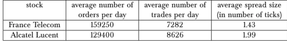
2.2 Data description and estimation of the reference price . . . 33
2.3 Model I: Collection of independent queues . . . 34
2.4 Model II: Dependent case . . . 37
2.5 Example of application: Probability of execution . . . 42
3 The queue-reactive model: a time consistent model with stochastic LOB and dynamic reference price . . . 43
3.1 Model III: The queue-reactive model . . . 43
3.2 Example of application: Order placement analysis . . . 46
4 Conclusion and perspectives . . . 49
5 Appendix . . . 50
5.1 Proof of Theorem 1 . . . 50
5.2 Computation of confidence intervals . . . 50
5.3 Quasi birth and death process . . . 51
5.4 Order Placement Tactic Analysis . . . 52
5.5 Alcatel-Lucent . . . 54
5.6 AES . . . 54
II A General Framework for Markovian Order Book Models 59 1 Introduction . . . 59
Contents
2 A general Markovian framework . . . 62
2.1 Representation of the order book . . . 62
2.2 Dynamics of the order book . . . 63
2.3 Comparison with existing models . . . 66
3 Ergodicity . . . 66
3.1 When pr e f stays constant . . . 67
3.2 General case . . . 69
4 Scaling limits . . . 70
5 Some specific models . . . 71
5.1 Best bid/best ask Poisson model (Cont and De Larrard (2013)) . . . 71
5.2 Poisson model withK > 1 . . . 72
5.3 Zero-intelligence model . . . 73
5.4 Queue-reactive model (Huang, Lehalle, and Rosenbaum (2013)) . . . 74
6 Conclusion . . . 75 7 Appendix . . . 76 7.1 Proof of Theorem 1 . . . 76 7.2 Proof of Theorem 2 . . . 78 7.3 Proof of Theorem 3 . . . 79 7.4 Proof of Theorem 5 . . . 80
Part II Tick Size Effects 83 III The Effect of Tick Value Changes on Market Microstructure: Analysis of the Japanese Experiements 2014 85 1 Introduction . . . 85
2 Cost of trading and high frequency price dynamics . . . 87
2.1 The model with uncertainty zones: When the tick prevents price discovery 87 2.2 Perceived tick size and cost of market orders . . . 88
2.3 Implicit bid-ask spread and cost of limit orders . . . 89
2.4 Prediction of the cost of market and limit orders . . . 90
2.5 What is a suitable tick value? . . . 91
3 Analysis of the Tokyo Stock Exchange pilot program on tick values . . . 91
3.1 Data description . . . 91
3.2 Classification of the stocks in Phase 0 . . . 92
3.3 Phase 0 - Phase 1 . . . 94
3.4 Phase 1 - Phase 2 . . . 95
4 Conclusion . . . 96
IV Intelligence and Randomness of Market Participants 99 1 Introduction . . . 99
2 Basic Model . . . 100
2.1 Price Dynamics . . . 100
2.2 Informed Trader, Noise Trader and Market Maker . . . 101
2.3 Some Assumptions . . . 102
2.4 Links between the Trade SizeQ, Price JumpB and the LOB Cumulative ShapeL(x). . . 102
2.5 The Bid-Ask Spread and the Equilibrium LOB Shape . . . 103
2.6 Variance per Trade . . . 106
Contents
3.1 Constrained Bid-Ask Spread . . . 107
3.2 Daily Volume . . . 110
3.3 Priority Value . . . 111
4 Examples . . . 111
4.1 Power-law Distributed Information . . . 111
5 Generalization . . . 112
5.1 How Information is Digested . . . 112
6 Conclusion and perspectives . . . 118
Bibliography 121
Introduction
In this thesis, we aim at building a general mathematical framework for order book modeling which enables us to link the macroscopic features of the price dynamics with the microscopic properties of the underlying asset. On the one hand, we want to shed light on some of the fundamental issues in order book modeling, such as the ergodicity of the order book and the role played by the tick value. On the other hand, our goal is also to provide relevant tools for market participants and regulators, helping them analyzing complex trading algorithms or effects of some regulatory measures.
Motivations
Can we explain the price dynamics of a stock from a microstructural point of view? This question is at the heart of market microstructure literature for decades. Many interesting results have been obtained and are nowadays used by practitioners as theoretical guidelines in the three main branches of high frequency trading: optimal execution, market making and statistical arbitrage. Such results usually aim at building a link between the high frequency dynamics of the the asset and the well established macroscopic features of the underlying stock. One of the most fascinating challenges in this context is to explain those links starting from the very finest microstructural scale, that of the limit order book. This limit order book modeling problem consists in establishing a tractable and relevant mathematical formulation for the market mechanics of order matching and order queueing, and for the complex behavior of market participants.
Although important advances have been made in the recent years about limit order book modeling, market participants still often find themselves in lack of applicable models when dealing with practical problems. In particular, in strong contrast to empirical findings, most existing limit order book models use an homogenous Poisson assumption on the order arrival process. Moreover, several models consider only the dynamics at the best bid/ask limits or assume constant bid-ask spread. These simplifications largely reduce the applicability of such models, as many algorithms used in practice operate on non-best limits and are very sensitive to their orders’ priority in the queue. Our goal being to provide relevant tools for market participants and regulators, the first question we want to address in this thesis is obviously the following one:
Question 1. How to build realistic order book models?
At the microscopic level, market activities are random and unpredictable. Yet when properly scaled in time, they exhibit many interesting regularities. For example, the price dynamics at the macroscopic level can be quite well approximated by a Brownian motion and the limit order book’s average shape tends to follow the same distribution across different trading days.
Introduction
This last regularity is closely related to the ergodicity of the limit order book system. In our first chapter, we introduce a state-dependent order book model, the queue-reactive model, that is particularly suitable for large tick assets1. This model is then extended to a more general Markovian framework, enabling us to deal with small tick assets and including most of the classical order book models. Thus we want to give an answer to the following important theoretical question for Markovian order book modeling:
Question 2. In a general Markovian framework for limit order book modeling, what are the required
conditions to obtain ergodic dynamics?
In our theoretical Markovian framework, market participants react differently under different market conditions. In the empirical study associated to the queue-reactive model, we find a strong contrast in traders behavior given various order book states, which validates our intuition that this state-dependent hypothesis is far more realistic than the traditional Poisson assumption. Interestingly, the estimated intensity functions for various assets for limit/market order insertion and limit order cancellation share many similarities. For example, the cancellation intensities are all found to be concave functions of the queue size, and the limit order insertion intensities at best limits tend to be essentially increasing functions. These common patterns can be seen as results of market participants intelligence. While they may be explained qualitatively by intuitive arguments such as the existence of market priority and risk of overrun, the following question remains very intricate:
Question 3. How to get a quantitative agent-based approach enabling us to understand the behavior
of market participants towards various states of the book and to retrieve the most important limit order book features?
One microstructural parameter having a strong influence on the trading practice of market participants is the tick value. We are particularly interested in this quantity since it is often considered the most relevant device to regulate the behavior of high frequency traders and to control market efficiency. Although several tick value change programs have been conducted in the recent years, most of them are designed using only empirical analysis and focus on the outcomes of the tick value modification in an ex post basis. Hence the effects of tick value changes have not been really understood and prediction tools enabling us to forecast the consequences of a tick value change are missing. Here we wish to fill this gap, with the aim to help market regulators to better determine the target tick values of such programs. Therefore we are considering the following question:
Question 4. How to predict the consequences of tick value changes?
Outline
This thesis is made of two main parts: order book modeling and tick size effects. Each question presented above corresponds to a chapter in one of these two parts.
In Part I, we present our work on order book modeling. In Chapter I, we answer Question 1 by building the queue-reactive model, in which state dependency is included in the order flow dynamics. We propose to split the order book modeling issue into two steps: i) dynamics of the order arrival processes around a constant reference price; ii) dynamics of the reference price. This enables us to design three different versions of the model, with various hypotheses on the
1A large tick asset is defined as an asset whose bid-ask spread is almost always equal to one tick.
1. Part I: Limit Order Book Modeling
information set used by market participants when making their trading decisions. Unlike the traditional Poisson assumption, order arrival intensities are assumed to be functions of the state of the order book. Estimation methods are provided and empirical studies are conducted on some large tick assets, showing that many macroscopic features can be explained adding state dependency in the order book dynamics. In particular, the distribution of the order book’s state is very well explained in this framework. We then show how to use this model as a market simulator for analyzing complex trading algorithms.
The answer to Question 2 is given in Chapter II. We first extend the queue-reactive model to a general Markovian framework, including most classical order book models. This new framework, while respecting the double-auction mechanism of the order book, imposes very little constraints. For example, the order size is allowed to be random, with distribution depending again on the order book’s state, and the reference price dynamics can also be linked to order book information such as the bid-ask imbalance. Ergodicity conditions in this framework are then discussed in details. Essentially, we show that if the incoming order flow (that is the limit order insertion rate) does not exceed the outgoing order flow (that is the sum of the market order and cancellation rates), then the order book state is an ergodic process. Furthermore, the price dynamics converges to a Brownian motion when properly rescaled.
Results about the role of the tick value are presented in Part II. To answer Question 4, we conduct in Chapter III an empirical study of the effects of tick value changes based on data from the Japanese tick size reduction pilot program between June 2013 and July 2014. We demonstrate that the approach introduced in Dayri and Rosenbaum (2012) allows for an ex ante assessment of the consequences of a tick value change on the microstructure of an asset. We focus on forecasting the future costs of market and limit orders after a tick value change and show that our predictions are very accurate. Furthermore, for each asset involved in the pilot program, we are able to define ex ante an optimal tick value.
We finally present in Chapter IV a preliminary attempt to answer Question 3. We split market par-ticipants into three types: informed traders, noise traders and market makers. Informed traders receive market information such as the current efficient price, which is hidden to noise traders. Market makers have also access to this information but with some delay, and they place limit orders when it is profitable. In a first model, we consider an idealized setting where the tick value constraint is removed, and assume that both informed traders and market makers have an infinite reaction speed to new information. In that case, we obtain a link between the price dynamics, the market volume and the equilibrium order book shape. We then study the effects of introducing the tick value constraint. We find that when the traded price becomes discrete, the priority value of a limit order can be properly defined and computed. Furthermore, the consequences of the uncertainty faced by market makers about the efficient price are discussed in our framework. We also provide insights on how a new piece of information is digested and propagated between informed traders and market makers and on the speed of order book recovery after a transaction. We now give a rapid overview of the main results obtained in this thesis.
1 Part I: Limit Order Book Modeling
Understanding the limit order book dynamics is one of the fundamental issues in modern electronic financial markets. Many practical problems, such as the design of a realistic market simulator and the performance evaluation of a high frequency trading algorithm, rely heavily on
Introduction
a reasonable limit order book model. Existing models often assume zero intelligence for market participants and focus only on dynamics at best limits, see for example Smith, Farmer, Gillemot, and Krishnamurthy (2003) and Cont and De Larrard (2013). This largely reduces their appeal for practice. In this part, we aim at building a complete order book model in which limits several ticks away from the best ones are considered and where market participants act in an intelligent way towards various order book states.
In Chapter I, we introduce the queue-reactive model for order book dynamics. The key idea in this model is to split the order book modeling issue into two parts: the order arrival dynamics during period of constant reference price and the dynamics of the reference price. This approach enables us to deal with the strong dependencies between the different limits and to study the sensitivity of the trading activities towards various order book states. We show that the queue-reactive model explains very well the asymptotic distribution of the order book and demonstrate its applicability to assess complex trading algorithms by conducting a detailed analysis of two order placement tactics. The ergodicity conditions of an extended Markovian order book framework are discussed in Chapter II. We prove that the rescaled price process converges to a Brownian motion and the order book state to an invariant distribution under some very general assumptions.
1.1 The Queue-reactive Model
1.1.1 Dynamics of the limit order book in a period of constant reference price
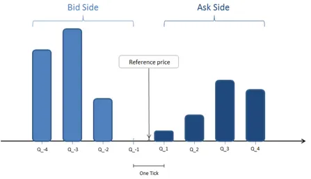
We model the limit order book as a2K dimensional vector, where K denotes the number of
available limits on the bid and ask side. By defining the reference pricepr e f as the center of
these2K limits and assuming it is constant, the limit order book dynamics can be described by a
continuous time Markov jump process X (t ) = (Q−K(t ), ...,Q−1(t ), ...,Q1(t ), ...,QK(t )), whereQi(t )
is the number of available orders at the i-th limit. The quantity pr e f can be viewed as some
current consensus price level and is used to index the limits. Three types of orders are considered: limit orders, cancellations and market orders, and their sizes are assumed to be constant for each limit (we set them here to one for simplicity). Under these assumptions, the infinitesimal generator matrix Qx,y of the process X (t ) can be written as follows (ei = (a−K, ..., ai, ..., aK),
whereaj= 0for j 6= i andai= 1):
Qq,q+ei = fi(q) Qq,q−ei = gi(q) Qq,q = − X p∈Ω,p6=q Qq,p Qq,p = 0,otherwise. Ergodicity conditions
WriteΩfor the state space ofq. The two following assumptions are needed for the ergodicity of
the process X (t ):
Assumption 1. (Negative individual drift) There exist a positive integerCbound andδ > 0, such
that for alli and all q ∈ Ω, ifqi> Cbound,
fi(q) − gi(q) < −δ.
1. Part I: Limit Order Book Modeling
Assumption 2. (Bound on the incoming flow) There exists a positive number H such that for any q ∈ Ω,
X
i ∈[−K ,...,−1,1,...,K ]
fi(q) ≤ H.
The first assumption states that the queue size of a limit should have a tendency to decrease when it becomes too large, while the second one ensures no explosion in the system. Under these two assumptions, we have the following ergodicity result for the2K-dimensional queuing
system with constant reference price, which will be the basis for our asymptotic study as well as for the estimation procedures.
Theorem 1. Under the above two assumptions, the 2K-dimensional Markov jump process X (t ) is ergodic.
Ergodicity conditions are discussed in more details in Chapter II.
The functions fi and gi model the state dependency of market participants’ behavior. Then
different assumptions on the information set used by traders lead to different models in the above framework. Three models are proposed to describe the order book dynamics under constant reference price.
Model I: Collection of independent queues
In Model I, we assume independence between the flows arriving at different limits:
fi(q) = λLi(qi) gi(q) = λCi(qi) + λMi (qi), whereλL i,λ C i ,λ M
i correspond to the intensities of limit orders, cancellations and market orders
respectively.
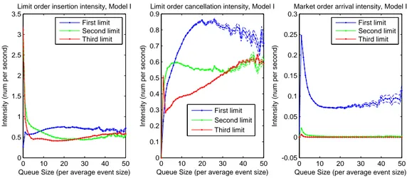
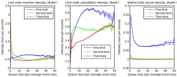
Model I enables us to study the influence of the target queue size on market participants’ behavior. In our empirical study conducted on large tick stocks, we find the following interesting repetitive patterns on the intensity functions (we takeK = 3in our experiments, the estimated
intensities for the stock France Telecom are shown in Figure .1): • Limit order insertion:
Q±1: The intensity of the limit order insertion process is approximately a constant function
of the queue size, with a significantly smaller value at 0. This can be explained by the fact that creating a new best limit is viewed as risky (inserting a limit order in an empty queue creates a new best limit and the market participant placing this order is the only one standing at this price level).
Q±2,3: The intensity is approximately a decreasing function of the queue size. This
interest-ing result probably reveals a quite common strategy used in practice: postinterest-ing orders at the second limit when the corresponding queue size is small to seize priority. • Limit order cancellation:
Q±1: In contrast to the classical hypothesis of linearly increasing cancellation rate, see for
example Cont, Stoikov, and Talreja (2010), the intensity of order cancellation is found to be an increasing concave function forQ±1. Such result can be explained by the
Introduction 0 10 20 30 40 50 0 0.5 1 1.5 2 2.5 3 3.5
Queue Size (per average event size)
In te n s it y ( n u m p e r s e c o n d )
Limit order insertion intensity, Model I First limit Second limit Third limit 0 10 20 30 40 50 0 0.1 0.2 0.3 0.4 0.5 0.6 0.7 0.8 0.9
Queue Size (per average event size)
In te n s it y ( n u m p e r s e c o n d )
Limit order cancellation intensity, Model I
First limit Second limit Third limit 0 10 20 30 40 50 -0.05 0 0.05 0.1 0.15 0.2 0.25 0.3
Queue Size (per average event size)
In te n s it y ( n u m p e r s e c o n d )
Market order arrival intensity, Model I First limit Second limit Third limit
Figure .1: Intensities atQ±i,i = 1, 2, 3, France Telecom
existence of the priority value, that is the advantage of a limit order compared with another limit order standing at the rear of the same queue. Actually, orders with lower priority are more likely to be canceled, see Gareche, Disdier, Kockelkoren, and Bouchaud (2013).
Q±2: The rate of order cancellation attains more rapidly its asymptotic value, which is
lower than that forQ±1. Compared to the first limit case, market participants at the
second limit have even stronger intention not to cancel their orders when the queue size increases. This is probably due to the fact that these orders are less exposed to short term market trends than those posted atQ±1 (since they are covered by the
volume standing atQ±1and their price level is farther away from the reference price).
Q±3: The priority value is smaller at the third limit since it takes longer time forQ±3 to
become the best quote if it does. The rate of order cancellation increases almost linearly.
• Market orders:
Q±1,2,3: The rate decreases exponentially with the available volume atQ±1,2,3. This
phenom-ena is easily explained by market participants “rushing for liquidity” when liquidity is rare, and “waiting for better price” when liquidity is abundant.
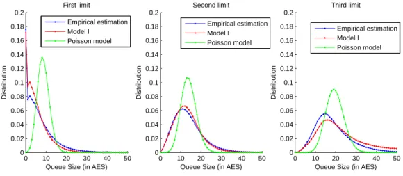
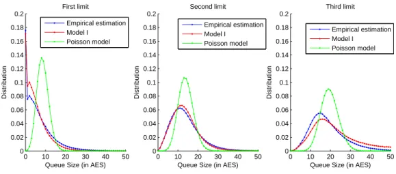
In Model I, each queue is actually a birth-death process whose invariant distribution can be computed explicitly: denote by πi the stationary distribution of the limit Qi, and define the
arrival/departure ratio vector ρi by
ρi(n) = λL i(n) (λCi(n + 1) + λiM(n + 1)). Then we have: πi(n) = πi(0) n Y j =1 ρi( j − 1) πi(0) = ¡1 + ∞ X n=1 n Y j =1 ρi( j − 1) ¢−1 . 6
1. Part I: Limit Order Book Modeling 0 10 20 30 40 50 0 0.02 0.04 0.06 0.08 0.1 0.12 0.14 0.16 0.18 0.2 First limit
Queue Size (in AES)
D is tr ib u ti o n 0 10 20 30 40 50 0 0.02 0.04 0.06 0.08 0.1 0.12 0.14 0.16 0.18 0.2 Second limit
Queue Size (in AES)
D is tr ib u ti o n 0 10 20 30 40 50 0 0.02 0.04 0.06 0.08 0.1 0.12 0.14 0.16 0.18 0.2 Third limit
Queue Size (in AES)
D is tr ib u ti o n Empirical estimation Model I Poisson model Empirical estimation Model I Poisson model Empirical estimation Model I Poisson model
Figure .2: Model I, invariant distributions of q±1, q±2, q±3, France Telecom
In Figure .2, we compare the theoretical asymptotic distributions with the empirical distributions observed at Q±1,Q±2,Q±3, and with the invariant distributions from a Poisson model with
constant limit/market order arrival rate and linear cancellation rate. The theoretical asymptotic distributions are found to be very good approximations of the empirical ones estimated from market data. This suggests that the empirical order book shape can be explained by the asymptotic equilibrium of order flow dynamics with state dependency.
Model II: Dependent case
In the dependent case, we differentiate best and non-best limits and also add dependence between the bid and ask limits. The generator of the process takes the following form:
fi(q) = λLi(q)
gi(q) = λCi(q) + λMbu y(q)1best ask(q)=i,ifi > 0
gi(q) = λCi(q) + λ M
sel l(q)1best bi d (q)=i,ifi < 0.
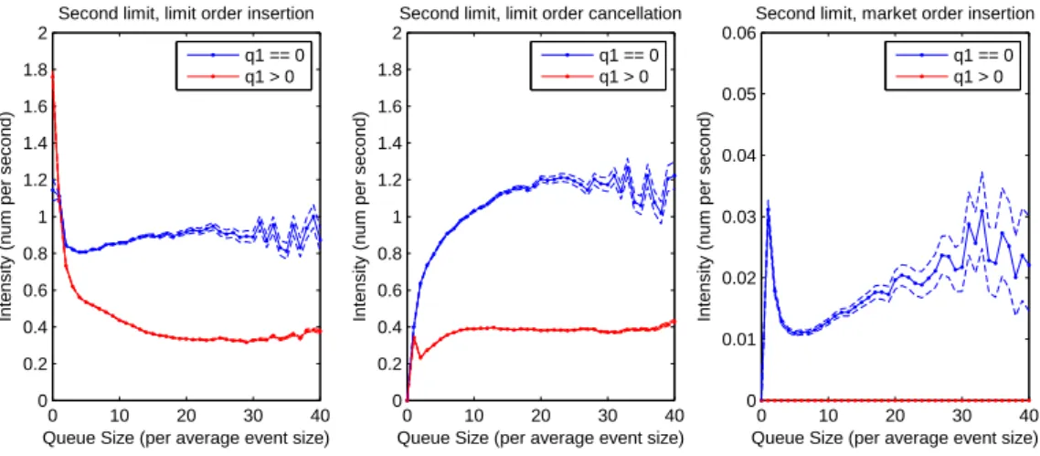
Model IIa: Two sets of dependent queues
In Model IIa, we propose to considerλL
±2 andλ
C
±2 as functions of q±2 and1q±1>0. Intensities at
Qi, i 6= ±2remain functions of qi only. Thus, in the empirical study of Model IIa, we focus on
understanding market participants’ behavior under two different situations: q±1= 0andq±1> 0.
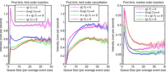
One of our interesting findings is the following one on the limit order arrival process:
• Limit order insertion: both intensities are decreasing functions of the queue size. In the first case (q±1= 0), the limit order insertion intensity reaches very rapidly its asymptotic
value. In the second case (q±1> 0), the intensity starts at a higher value for q2= 0but
continues to go down to a much lower value. This is likely related to the following arbitrage strategy: post passive orders at a non-best limit when its size is small, wait for this limit to eventually become the best limit and then gain the profit from having the priority value. For example, when the considered limit becomes the best one, one can decide to stay in the queue if its size is large enough to cover the risk of short term market trend, or to cancel the orders if the queue size is too small.
Introduction
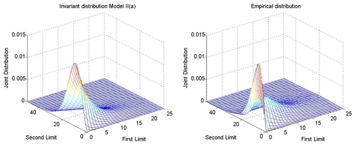
The joint asymptotic distribution for the limit order book state(q1, q2)can be computed
nu-merically in Model IIa, using the fact that it is a quasi-birth-and-death process, see Latouche
and Ramaswami (1999), and is found to be again a very good approximation of the empirical one. Model IIb: Modeling the bid-ask dependences
To study the interactions between the bid side and the ask side, we define the functionSm,l(x)
for representing four different ranges of values for the queue sizes (empty, small, usual and large):
Sm,l(x) = Q0 ifx = 0
Sm,l(x) = Q− if0 < x ≤ m
Sm,l(x) = Q¯ ifm < x ≤ l
Sm,l(x) = Q+ ifx > l ,
for well chosenm andl.
In Model IIb, market participants atQ
±1 adjust their behavior not only according to the target
queue size, but also to the size of the opposite queue. The ratesλL
±1 andλ
C
±1 are thus modeled
as functions ofq±1 andSm,l(q∓1). Regime switching atQ±2 is kept in this model:λL±2,λC±2are
assumed to be functions of q±2 and 1q±1>0.
Some remarks are in order:
• Limit order insertion: the limit order insertion rate is a decreasing function of the opposite queue size. In particular, when the opposite queue is empty, it is significantly larger. Indeed, in that case, the “efficient" price is likely to be closer to the opposite side. Therefore limit orders at the non empty first limit are likely to be profitable.
• Limit order cancellation: the cancellation rates for different ranges ofQ−1 are similar in
their forms but have different asymptotic values. This rate is not surprisingly a decreasing function of the liquidity level on the opposite side. Indeed, when this level becomes low, many market participants cancel their limit orders and send market orders since the market is likely to move in an unfavorable direction.
• Market orders: we see that when the liquidity available on the opposite side is abundant, more market orders are sent. Indeed, in that case, transactions at the target queue are relatively cheap as its price level is temporarily closer to the efficient price. In the special situationq−1= 0, the price level atQ1can seem relatively attractive since it is much closer
to the reference price than the opposite best price, which is in that case 1.5 ticks away from it. This explains why the market order intensity is larger when the opposite queue is empty than when its size is small.
Invariant distributions for the limit order book in Model IIb can be obtained using
Monte-Carlo simulations, and the comparison results with the empirically estimated ones are still very satisfactory.
1. Part I: Limit Order Book Modeling
1.1.2 A time consistent model with stochastic limit order book and dynamic reference price
We then propose a model accommodating a dynamic limit order book center: the queue-reactive model.
The queue-reactive model
Dynamics of the reference price is added by linkingpr e f with the mid pricepmi d: we assume
that changes ofpr e f are triggered by changes of the mid price with some probabilityθ. We also
add another parameterθr ei ni t to incorporate price jumps resulting from external information:
in such case, the order book state is redrawn from some invariant distribution around the new reference price. These two parameters are calibrated using10min price volatility and the mean
reversion ratioηfrom Robert and Rosenbaum (2011). Maximum mechanical volatility
Whenθr ei ni t
= 0, price fluctuations are only endogenously generated by the order book dynamics.
In such case, the volatility is an increasing function ofθ and attains its maximum value when
θ = 1. The associated volatility is called maximum mechanical volatility, and is found to be often
smaller than the empirical volatility, which justifies the use of the parameterθr ei ni t.
1.1.3 Order placement analysis
In practice, an execution algorithm gives answers to the two following questions:
• Order Scheduling: how to distribute the target volume across the trading horizon? • Order Placement: how to send individual orders to the order book?
The first question is widely studied in the literature, see for example Bertsimas, Lo, and Hummel (1999); Almgren and Chriss (2000); Bouchard, Dang, and Lehalle (2011). Answers to it often rely on some “optimal trading curve”, which depends mainly on intraday factors such as the average volume curve, the intraday volatility and the average market impact profile. The second question can be seen as the microstructural version of the first one, but is much more difficult to solve since the dynamics are more complex. Related academic works address the problem of determining the optimal order type (whether to send limit or market order) Harris and Hasbrouck (1996), or of finding the best position to place the order Laruelle, Lehalle, and Pagès (2013). In practice, order placement tactics are usually much more complex.
While most existing approaches for post-trade performance analysis focus on the overall per-formance, it is actually more reasonable to separate the order scheduling part from the order placement part. Performance of order placement tactics depends more on ultra-high frequency features such as the latency, the queue priority, bid-ask imbalance, etc, which have generally little influences over the choice of the “optimal trading curve”. Moreover, the same order scheduling strategy can be coupled with different order placement tactics to build different execution algorithms. In such cases, it is important to be able to understand the pros and cons of each placement tactic so that an informed choice can be made to determine the best tactic under different market conditions.
Introduction
We present in this introduction an application example to show how the queue-reactive model can be used in the context of order placement analysis for sophisticated tactics.
Denote ntot al for the total quantity to execute and M for the number of trading slices. An
order scheduling strategy gives the target quantity to be executed in each slice, denoted by ni
(PM
i =1ni= ntot al). Two types of order scheduling strategies, denoted by S1 and S2, are considered
in this example:
• S1: A linear scheduling (ni= ntot al/M), used for the VWAPbenchmark (volume weighted
average price).
• S2: An exponential scheduling ni= ntot al(e−(i −1)/4− e−i /4), used for the benchmarkS0
(arrival price).
An order placement tactic can be seen as a predefined procedure of order management, ensuring the execution of the target quantity within the slice. The following two tactics will be considered in our analysis: in the i-th slice, both tactics post a limit order of sizeni at the best offer queue
at the beginning of the period, and send a market order with all the remaining quantity to complete the execution of the target volume at the end time of the slice. In between:
• T1 (Fire and forget): When pmi d (the mid price) changes, cancel the limit order and send
a market order on the opposite side with all the remaining volume if any.
• T2 (Pegging to the best): When the best offer price changes or our order is the only remaining order at the best offer limit, cancel the order and repost all the remaining volume at the newly revealed best offer queue.
Performance measure
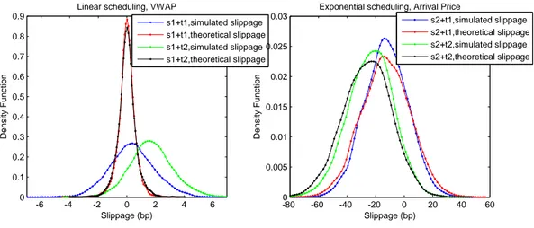
To understand the effects of order placement tactic on the execution’s slippage, we propose the two following measures on an execution’s performance: Slippage and Slippaget heo.
Slippage = Pbenchmar k− Pexec
Pbenchmar k , Slippaget heo = Pbenchmar k− P t heo exec Pbenchmar k ,
wherePexect heo=PM
i =1niVWAPi represents the average execution price if the algorithm obtains the
same price as the market VWAP in each trading slice. Essentially, Slippage measures the overall performance of the execution algorithm as a combination of order placement tactic and order scheduling strategy, while Slippaget heo measures the quality of the scheduling strategy alone and
neglects the randomness in executed price due to the order placement tactic in each trading slice.
2000simulations are launched for each couple of (S1/S2, T1/T2). We then estimate the probability
density functions of Slippaget heo and Slippage. The results are shown in Figure .3. The
simulation results suggest that the same order scheduling strategy can have very different performance when being coupled with different order placement tactics: T2 (“Pegging to the best”) performs better than T1 (“Fire and forget”) when being coupled with a linear scheduling strategy with VWAP benchmark, while T1 slightly outperforms T2 when an exponential scheduling strategy with arrival price benchmark is considered. By executing most of the target quantity via limit orders, T2 obtains on average a better price than that of a more market orders based
1. Part I: Limit Order Book Modeling -6 -4 -2 0 2 4 6 0 0.1 0.2 0.3 0.4 0.5 0.6 0.7 0.8 0.9 Slippage (bp) D e n s it y F u n c ti o n
Linear scheduling, VWAP
s1+t1,simulated slippage s1+t1,theoretical slippage s1+t2,simulated slippage s1+t2,theoretical slippage -80 -60 -40 -20 0 20 40 60 0 0.005 0.01 0.015 0.02 0.025 0.03 Slippage (bp) D e n s it y F u n c ti o n
Exponential scheduling, Arrival Price
s2+t1,simulated slippage s2+t1,theoretical slippage s2+t2,simulated slippage s2+t2,theoretical slippage
Figure .3: Simulation results for the tactics
tactic. However, at the same time, it creates a larger impact than T1 since the order stays longer in the queues. Note that market impact profiles for these two tactics can also be obtained using Monte-Carlo simulations.
1.2 A General Framework for Markovian Order Book Modeling
In Chapter II, we extend the queue-reactive model to a general Markovian framework. 1.2.1 Order book dynamics
We represent the order bookX (t ) by two elements: its center position denoted bypr e f (which
plays the same role as pr e f in the queue-reactive model) and its form [q−K, ..., q−1, q1, ..., qK].
The use of one unique reference price that is not directly observable from the order book state gives us flexibility for modeling the order book and enables us to differentiate two types of jumps in the order book dynamics: pure order book state jumps (for which the order book cen-terpr e f stays invariant) and common jumps (jumps in which a reference price change is involved).
Pure order book jump
We assume that a pure order book jump can only happen at one specific queue at each jump time. Unlike the queue-reactive model, buy/sell limit orders are allowed to be inserted on both parts of the reference price. Moreover, the jump size is now random. Thus, in term of generator, we have, with 2K functions fi, gi:
Q(q,p),(q+nei,p) = fi(q, n) Q(q,p),(q−nei,p) = gi(q, n)
˜
Q(q,p),(q0,p) = 0, otherwise. Common jump
New information such as the arrival of a market order may affect the value of the consensus price, and such effect takes place with some delay in practice. In our framework, we use a
Introduction
discretizedpr e f (with tick value denoted byα) and model the jump rate ofpr e f as function of
the order book state q(t ):
X q0∈Ω Q(q,p),(q0,p+α) = u(q) X q0∈Ω Q(q,p),(q0,p−α) = d(q) X q0∈Ω Q(q,p),(q0,p±nα) = 0, forn ≥ 2.
Note that when the order book center changes, the values of qi switches immediately to the
value of one of its neighbors. We thus introduce two boundary distributionsπ−K andπK for
generating new queue sizes atQ±K as we keep onlyK limits on each side. As in the
queue-reactive model, we assume thatq±K is redrawn from some distribution (πi nc ifpr e f increases,
πd ec if it decreases) with some probability θr ei ni t whenever a reference price jump happens.
For q ∈ Ω (Ω denotes the state space of all possible order book shape) andl ∈ R, write q+=
[q−K, ..., q−1, q1, ..., qK −1],q−= [q−K −1, ..., q−1, q1, ..., qK],[q+, l ] = [q−K, ..., q−1, q1, ..., qK −1, l ]and
[l , q−] = [l , q−K −1, ..., q−1, q1, ..., qK]. We have for any q, q0, q00such thatq0+6= q+ andq00−6= q−:
Q(q,p),([q+,l ],p+α) = (1 − θr ei ni t)u(q)πK(l ) + θr ei ni tu(q)πi nc([q+, l ]) Q(q,p),(q0,p+α) = θr ei ni tu(q)πi nc(q0)
Q(q,p),([l ,q−],p−α) = (1 − θr ei ni t)d (q)π−K(l ) + θr ei ni td (q)πd ec([l , q−]) Q(q,p),(q00,p−α) = θr ei ni td (q)πd ec(q00).
The infinitesimal generator matrix of the order book process
Gathering all the above hypotheses together, we obtain the following description for the infinites-imal generator matrix of the Markovian jump process X (t ):
Assumption 3. For anyq, q0, q00, ˜q ∈ Ω, p, ˜p ∈ α(0.5 + Z),n ∈ N+,l ∈ Z, such that q0+6= q+ and
q00−6= q− , the infinitesimal generator matrix Q of the process X (t ) is of the following form (with
2K functions fi, gi:Ω × N+→ R+and2functions u, d :Ω → R+) :
Q(q,p),(q+nei,p) = fi(q, n) Q(q,p),(q−nei,p) = gi(q, n) Q(q,p),([q+,l ],p+α) = (1 − θr ei ni t)u(q)πK(l ) + θr ei ni tu(q)πi nc([q+, l ]) Q(q,p),(q0,p+α) = θr ei ni tu(q)πi nc(q0) Q(q,p),([l ,q−],p−α) = (1 − θr ei ni t)d (q)π−K(l ) + θr ei ni td (q)πd ec([l , q−]) Q(q,p),(q00,p−α) = θr ei ni td (q)πd ec(q00) Q(q,p),(q,p) = − X ( ˜q, ˜p)∈Ω×α(0.5+Z),( ˜q, ˜p)6=(q,p) Q(q,p),( ˜q, ˜p) Q(q,p),( ˜q, ˜p) = 0,otherwise.
Note that up to minor modifications, most classical order book models such as the zero-intelligence model of Smith et al. (2003) and that of Cont et al. (2010), and the queue-reactive model, can be included in this framework.
1.2.2 V-Uniform ergodicity Constant reference price
1. Part I: Limit Order Book Modeling
We now discuss ergodicity conditions for the Markovian process X (t ). V-uniform ergodicity
implies the existence of a unique invariant distribution for the state vectorq(t ), which is very
useful in explaining the empirical order book distribution, as we have already seen in the queue-reactive model. We write
fi∗(q) :=X n fi(q, n), gi∗(q) :=X n gi(q, n),
and consider two probability measures onN+
li(q, n) := fi(q, n) f∗ i (q) , ki(q, n) := gi(q, n) g∗ i(q) ,
and their related moment-generating functionsGf ,i ,q(z)andGg ,i ,q(z). We make the following
assumptions:
Assumption 4. For any order book stateq and anyi ≥ ibest ask,gi(q, n) = 0for anyn > qi and for
any order book stateq and anyi ≤ ibest bi d, fi(q, n) = 0for anyn > −qi.
Assumption 5. There existsz∗> 1such that for any q andi,Gf ,i ,q(z∗) < ∞andGg ,i ,q(z∗) < ∞.
Furthermore, there existsL > 0such that for anyi,
lim
z→1+supq [ f
∗
i (q)Gf ,i ,q(z)1i >ibest bi d+ g
∗
i(q)Gg ,i ,q(z)1i <ibest ask] < L.
Assumption 6. There existr > 0andU > 1such that
lim
z→1+ sup
(q,i ):qi>U ,i ≥ibest ask
[ fi∗(q) − gi∗(q)
1 −Gg ,i ,q(z−1)
Gf ,i ,q(z) − 1 ] < −r
lim
z→1+ sup
(q,i ):qi<−U ,i ≤ibest bi d
[gi∗(q) − fi∗(q)
1 −Gf ,i ,q(z−1)
Gg ,i ,q(z) − 1 ] < −r.
Assumption 7. For anyz > 1,
Bf(z) := inf
(q,i ):qi>U ,i ≥ibest ask
(Gf ,i ,q(z) − 1) > 0
Bg(z) := inf
(q,i ):qi<−U ,i ≤ibest bi d
(Gg ,i ,q(z) − 1) > 0.
Under these assumptions, we have the following result:
Theorem 2. When u = d ≡ 0, under Assumption 4, 5, 6 and 7, the continuous-time Markov jump
Introduction
For the embedded Markov chain q(n), defined as q(n) = q(Jn), with Jn the time of the n-th
jump, andq(Jn)the state of the LOB after this event, a different assumption is needed for its
ergodicity. We write a∗i(q) = f ∗ i (q) P i[ fi∗(q) + gi∗(q)] , b∗i(q) = g ∗ i(q) P i[ fi∗(q) + gi∗(q)] ,
for the proportions of queue size increases and decreases, and replace Assumption 6 by the following one.
Assumption 8. There existr > 0andU > 1such that
lim
z→1+(q,i ):q sup
i>U ,i ≥ibest ask
[a∗i(q) − bi∗(q)1 −G
g ,i ,q(z−1)
Gf ,i ,q(z) − 1 ] < −r
lim
z→1+(q,i ):q sup
i<−U ,i ≤ibest bi d
[bi∗(q) − ai∗(q)1 −G
f ,i ,q(z−1)
Gg ,i ,q(z) − 1 ] < −r.
Then we can prove the following theorem:
Theorem 3. Whenu = d ≡ 0, under Assumptions 4, 5, 7 and 8, the embedded discrete-time Markov
chain q(n)is V-uniformly ergodic and positive Harris recurrent.
The main idea to prove the ergodicity ofq is to design an appropriate Lyapunov functionV, on
which the following negative drift condition is satisfied for someγ > 0 andB > 0:
QV (q) := X
q06=q
Qq q0[V (q0) − V (q)] ≤ −γV (q) + B.
Then the above theorems can be derived using Theorem 4.2 and Theorem 6.1 in Meyn and Tweedie (1993). Note that the same kind of method is used in Abergel and Jedidi (2011) in order to show ergodicity properties of zero-intelligence order book models.
General case For somez,U > 1, let
Vz([q, c]) =
K
X
i =−K ,i 6=0
z|qi|−U.
Whenpr e f is no longer constant, we make the two following additional assumptions:
Assumption 9. There exist z > 1 and Lπ> 0 such that forQi nc, Qd ec, QK, Q−K four random
variables such thatQi nc∼ πi nc,Qd ec∼ πd ec,QK ∼ πK andQ−K∼ π−K:
E[Vz([Qi nc
, c])] + E[Vz([Qd ec, c])] + E[z|QK|−U] + E[z|Q−K|−U] ≤ Lπ.
Assumption 10. There exists a finite setW ⊂ Ω such that the upper bound of the proportion of
reference price jumps in any order book stateq is smaller than one onΩ/W:
sup q∈Ω/W u(q) + d(q) P i[ fi∗(q) + gi∗(q)] + u(q) + d(q)< 1. 14
1. Part I: Limit Order Book Modeling
Recall thatq(n)represents the state of the order book after the n-th event and pr e f(n)is the
reference price after the n-th event, we consider here the process of reference price increments
c(n), defined as the reference price change at the n-th event:
c(n) = pr e f(n) − pr e f(n − 1).
We have the following theorem on the ergodicity of the Markov chainY (n) = (q(n),c(n)):
Theorem 4. Under Assumptions 4, 5, 7, 8, 9 and 10, the embedded discrete-time Markov chain
Y (n) = (q(n),c(n))is V-uniformly ergodic and positive Harris recurrent.
1.2.3 Scaling limit
Another important element in order book modeling is the scaling limit of the price process. Let
N (t ) = inf{n, Jn≤ t }
be the number of events until timet, with the conventioninf{;} = 0. Let Z (n)be the cumulative
price change until then-th event, that isZ (0) = 0and forn ≥ 1:
Z (n) = n X i =1 c(i ). We have Z (N (t )) = pr e f(t ) − pr e f(0).
Thus it represents the reference price at time t recentered its starting value. The following
theorem shows that the rescaled price process Sˆ(n)
(t ) := Z (bntc)p
n in event time converges to a
Brownian motion under the preceding assumptions:
Theorem 5. Under Assumptions 4, 5, 7, 8, 9 and 10, ifEπ∗[c(0)] = 0, then the series
σ2 = Eπ∗[c02] + 2 ∞ X n=1 Eπ∗[c0cn],
converges absolutely, withπ∗ the invariant distribution of(q(n), c(n)). Furthermore, if Y (0) ∼ π∗,
we have the following convergence in law inD[0, ∞):
ˆ
S(n)(t )n→∞→ σB(t ),
whereB (t )is a standard Brownian motion.
Consider now the following additional assumption: Assumption 11. There exists somem > 0, such that
inf
q∈Ω
© X
i
( fi∗(q) + gi∗(q)) + u(q) + d(q)ª > m.
Then we have the following result on the convergence of the rescaled reference price process in calendar time:
˜
S(n)(t ) =Z¡N (nt)¢p
Introduction
Theorem 6. Letτnbe the inter-arrival time between then-th and the(n−1)-th jumps of the Markov
processX. Under Assumptions, 4, 5, 7, 8, 9, 10 and 11, the process(q(n), c(n),τ(n))is positive Harris
recurrent. Furthermore, ifEπ∗[c(0)] = 0andY (0) ∼ π∗, then ˜
S(n)(t )n→∞→ p σ
Eπ∗∗[τ(1)]
B (t ),
withπ∗∗ the invariant distribution of(q(n), c(n),τ(n)).
The above two theorems discuss the scaling limit of the underlying reference price process. For the more usual process such aspbest bi d(t ),pbest ask(t )andpmi d(t ), the same result still apply
since they are all bounded by 2K with respect topr e f(t ).
2 Part II: Tick Value Effects
The tick value is the minimum price change imposed by the market designer on a traded asset. It is one of the most important structural parameters that affect the microstructure of the underlying asset and thus its macroscopic properties. In this part, we present our theoretical and empirical results in studying the role of tick size in high frequency trading.
2.1 The Effects of Tick Value Changes on Market Microstructure: Analysis of the 2014 Japanese Experiment
In Chapter III, we study the effects of tick value reduction for large tick assets. We aim at demonstrating that the approach introduced in Dayri and Rosenbaum (2012) allows for an ex
ante assessment of the consequences of a tick value change on the microstructure of a large
tick asset. The data of the Japanese tick value reduction pilot program are analyzed in light of this methodology. For these assets, the notion of implicit spread is introduced using the high frequency indicatorηfrom the model with uncertainty zones of Robert and Rosenbaum (2011). This enables us to forecast the future cost of market and limit orders after a tick value change. Our results are shown to be very accurate. Furthermore, we are able to define an “optimal tick value” for each asset that helps classify the assets according to the relevance of their tick value, before and after its modification.
2.1.1 Cost of trading and high frequency price dynamics The high frequency indicatorη
We propose to use a unique high frequency indicator, the parameterη (which can be easily estimated), to summarize the high frequency features of the asset. This indicator, already used in the queue-reactive model for calibration purpose, allows us to build an estimate for the relative cost of market orders and limit orders, and is directly linked to the tick size. In the first part of this chapter, we show why this indicator is far more subtle and suitable for microstructure analysis than any other measurement, like the ones based on the conventional bid-ask spread or on the market depth.
The model with uncertainty zones assumes the existence of a latent efficient price processXt,
and that a transaction at a certain price level can happen only when the price level is close enough to the efficient price. This proximity is quantified by the parameter η: the distance between the possible transaction price and the efficient price must be smaller than α(1/2 + η),
2. Part II: Tick Value Effects
withαthe asset’s tick value. The zone with width2ηαaround the mid price is called uncertainty
zone. When the efficient price is inside it, both buy and sell market orders can occur. Perceived tick size and cost of market orders
The parameterηmeasures the mean-reversion level of the transaction price due to the existence of the tick value. For large tick assets,ηis also related to the perceived tick size of the asset by market participants: a smallη(< 0.5) means that the tick value appears too large while a large
η(> 0.5) means that it is considered too small, see Dayri and Rosenbaum (2012). Knowingη
also enables us to compute the cost of the orders. Take for example a market order at pricePt
leading to an upward price change at timet. The ex post expected cost of this order is given by: Pt− E[X∞|Xt] = α/2 − ηα.
Prediction of the cost of market and limit orders
Let us consider a large tick asset with current tick value α0 and associated high frequency
indicator η0. When the tick value is changed to α, the following prediction formula for the
new value ofη(and thus the cost of market and limit orders) can be established based on the invariance of the volatility with respect to the tick value:
η ∼ (η0+ 0.1)(α0
α)
1/2
− 0.1. (1)
This formula, which is valid for large tick assets(η ≤ 0.5), enables us:
• To tell whether the asset will remain a large tick asset after the tick value change: if the
predicted value ofηis greater or equal than0.5, the asset is predicted to become a small
tick asset after the tick value change.
• To predict the new value ofη: if the predicted value ofηis smaller than0.5, the above
formula computes the estimatedηafter the tick value change. The optimal tick value
Being able to predict the value ofηafter a tick value change not only helps the market designer to forecast the consequences of their measures on the market microstructure, but also paves the way for defining a notion of “optimal tick value”. Although different market participants can have quite opposite views on what a good tick value is, there are in general two main objectives in a tick value change program:
• The bid-ask spread should be close to one tick, ensuring the presence of liquidity in the order book.
• Transaction costs should be close to zero for market orders. In that case, the market is efficient and market makers do not take advantage of the tick value to the detriment of final investors acting mainly as liquidity takers.
In our approach, an asset enjoys a relevant tick value if it is a large tick asset and itsηparameter is close to1/2. Thus we have the following formula for the optimal tick value:
αop t=α0
(η0+ 0.1)2
Introduction
2.1.2 Analysis of the Tokyo stock exchange pilot program on tick values
The Tokyo stock exchange pilot program, in which 55 stocks are involved in a tick size reduction plan, consists in three phases: Phase 0 (before the pilot program), from June 3, 2013 to January 13, 2014; Phase 1 (between the first and the second implementation of the tick value reduction program), from January 14, 2014 to July 21, 2014; Phase 2 (after the implementation of the second tick value reduction program), from July 22, 2014 to December 30, 2014. We assess the quality of the prediction formula on this experiment by predicting the outcomes of the first and second tick value reductions and comparing our forecasts to the empirical results.
Classification of the stocks
The 55 stocks are classified according to their conventional spreadS (in ticks) and to the level of
market order cost. We first split the stocks into three groups:
• Small tick stocks: S > 1.6.
• Large tick stocks: S ≤ 1.5.
• Ambiguous cases: 1.5 < S ≤ 1.6.
The cost of market order beingα/2 − ηα, we use the high frequency indicatorηto distinguish between balanced stocks (for which the cost of market order is close to0) and market makers
favorable stocks (where market makers obtain significant profit from liquidity takers thanks to the large tick value):
• Balanced stocks: η ≥ 0.4.
• Market makers favorable stocks: η < 0.4.
A stock is considered to have a “suitable” tick value if it is both a large tick stock and a balanced stock. Note that all small tick stocks are considered as balanced stocks, but they do not have “suitable” tick value, their bid-ask spread (in ticks) being too large. Among the55stocks involved
in the pilot program, only 5of them are considered having a suitable tick value before the start
of the program. This means that a tick value modification can be beneficial for the other 50
stocks.
Phase 0 - Phase 1
During Phase 1, 12 stocks being large tick assets in Phase 0 are involved in the tick value
reduction program. These stocks are selected to test the prediction quality of Formula 1 on the new value ofηin Phase 1 (ηp1). The predicted valueη
p
1 tells directly whether the asset will remain
a large tick asset and whether it will be balanced after the tick value modification. We use the following criteria:
• Ifηp1≥ 0.55, the asset is predicted to become a small tick asset after the tick value change.
• Ifηp1< 0.5, the asset is predicted to remain a large tick asset after the tick value change,
with the forecast value for the newηbeing meaningful and given byηp
1.
• We qualify the situation 0.5 ≤ ηp1< 0.55as an “ambiguous” case between large tick and
small tick.
2. Part II: Tick Value Effects
We obtain an average relative prediction error for ηof 18% along with very tight confidence
intervals for these12stocks in Phase 1. Having such accurate predictions, it is no surprise that
we are also able to forecast the category an asset will belong to after the tick value modification with very high success rate (only 2 errors).
Phase 1 - Phase 2
More stocks (48) are affected in Phase 2 by the tick value reduction program. For these stocks, we
conduct a similar analysis as the one for Phase 0 - Phase 1. An excellent accuracy is once again obtained for the prediction ofηand the category of these stocks after the tick value modification: the average relative prediction error is reported to be less than17%, with a success rate of85%
for the prediction of the stock’s category. These results confirm the excellent prediction quality of Formula 1 and the ability of our methodology to forecast ex ante the consequences of a tick value change on the microscopic properties of the asset.
2.2 An Agent-based Model on Order Book Dynamics
In Chapter IV, we introduce a simple agent-based model on order book dynamics, which gives insights on the relationships between traded volumeV, price volatilityσ, tick sizeα, bid-ask
spreadφand the order book equilibrium formL(x)(L(x)denotes the quantities of buying/selling
orders between P (t ) and P (t ) + x, where P (t ) denotes the market underlying efficient price,
whose role is equivalent to the role ofpr e f in Part I).
2.2.1 Model with infinitesimal tick size
We assume that P (t ) = P0+ Y (t ), with Y (t ) a compound Poisson process with jump rate λi
and size (denoted by B) distribution ψ (defined on R). We impose E[B] = 0 so that P (t ) is
a martingale. In such case, we have σ := V[P(t)]t = λiE[B2], where the term σ represents the
macroscopic volatility. Agents
We assume that there exist three types of traders in the market:
• One informed trader: the informed trader receives the value of the price jump sizeB right
before it happens. He then sends his trades based on this information to gain profit. We assume that he can only send market orders.
• One noise trader: the noise trader sends random market orders to the market. We assume
that these trades follows a compound Poisson process, with arrival rateλu and volume
distributionκu in R(positive volume represents a buying order, while negative volume
represents a selling order).
• Market makers: the market makers receive the value of the price jump sizeB right after it
happens. They place limit orders and try to make profit. We assume that they are risk neutral.
The following greedy assumption on the informed trader’s behavior enables us to link the informed trader’s trade sizeQi, the noise trader’s trade sizeQu, the price jump sizeB and the