ÉCOLE DE TECHNOLOGIE SUPÉRIEURE UNIVERSITÉ DU QUÉBEC
THESIS PRESENTED TO
ÉCOLE DE TECHNOLOGIE SUPÉRIEURE
IN PARTIAL FULFILLMENT OF THE REQUIREMENTS FOR THE DEGREE OF DOCTOR OF PHILOSOPHY
Ph.D.
BY
Mamadou Kabirou TOURÉ
STABILISED LEVEL SET METHODS FOR TWO-PHASE FLOW SIMULATION
MONTREAL, NOVEMBER 1, 2016
This Creative Commons licence allows readers to download this work and share it with others as long as the author is credited. The content of this work may not be modified in any way or used commercially.
BOARD OF EXAMINERS (THESIS PH.D.) THIS THESIS HAS BEEN EVALUATED BY THE FOLLOWING BOARD OF EXAMINERS
Mr. Azzeddine Soulaïmani, Thesis Supervisor
Department of Mechanical Engineering at École de technologie supérieure
Mr. Ammar Kouki, Chair, Board of Examiners
Department of Electrical Engineering at École de technologie supérieure
Mr. Stéphane Hallé, Member of the Jury
Department of Mechanical Engineering at École de technologie supérieure
Mr. Wahid Ghaly, External Evaluator
Department of Mechanical and Industrial Engineering at Concordia University, Montreal, Canada
THIS THESIS WAS PRESENTED AND DEFENDED
IN THE PRESENCE OF A BOARD OF EXAMINERS AND THE PUBLIC ON OCTOBER 18, 2016
ACKNOWLEDGMENTS
This thesis is the result of many years of work at the “École de technologie supérieure” (ÉTS) in Montreal. This work was carried out within the research unit “Groupe de Recherche sur les Applications Numériques en Ingénierie et en Technologie” (GRANIT) dedicated to the research and development of numerical methods for the mathematical modelling and numerical simulation of multiphysics problems.
Many people have contributed to or helped in some way with the completion of this doctoral thesis. First, I would like to thank my supervisor, Professor Azzeddine Soulaïmani, Ph.D., for giving me the opportunity to carry out the research throughout this thesis within the GRANIT research group by providing me excellent working conditions and support.
Furthermore, I would like to thank all my colleagues of the GRANIT research group for their scientific and technical contributions to this project: their discussions have always been helpful, particularly in the area of multiphase flows.
Moreover, I would like to express my gratitude to all of those who have supported me during my studies and have encouraged me to bring this project to term, especially my mother Suzanne Kadidja Fau, a career teacher; my late father Professor Alioune Touré at “École Normale Supérieure d’Enseignement Technique et Professionnel” (ENSETP), affiliated with “Université Cheikh Anta Diop de Dakar” (UCAD); and my two grand sisters Coumba Touré and Marième Touré.
MÉTHODES DE LEVEL SET STABILISÉES POUR LA SIMULATION D’ÉCOULEMENT DIPHASIQUE
Mamadou Kabirou TOURÉ
RÉSUMÉ
Ce travail est consacré à la simulation numérique des écoulements diphasiques incompressibles en utilisant un champ de vitesse imposé ou obtenu à partir d’un solveur Navier-stokes. L'objectif principal est de retracer précisément l’interface entre deux phases fluides d’un domaine qui est soumis à un champ de vitesse. L’application de ce type de problème se retrouve aisément dans les écoulements en surface libre, les conduites où s’écoulent un mélange de liquides et des bulles de gaz ou bien un mélange de deux liquides immiscibles tels que l’eau et l’huile. Nous avons déterminé la position de l’interface entre deux phases par la méthode des lignes de niveaux (« level set method ») qui consiste à résoudre une équation de transport à laquelle nous avons ajouté un terme de stabilisation qui réduit d’une manière globale l’erreur de la position de l’interface au cours de la simulation. Cette nouvelle classe de méthode d'éléments finis proposée a permis de résoudre le problème de transport d'interface en se basant sur l'approche de la méthode « level set ». La formulation peut, dans certains cas simples, produire une solution de l’interface précise sans avoir recours à la procédure de réinitialisation. Cependant dans d’autres cas d’écoulement plus complexes, les méthodes stabilisées proposées utilisées avec la méthode de réinitialisation géométrique permettent d’éliminer les oscillations. Dans la première partie de notre étude, nous avons obtenu les formulations proposées en ajoutant un terme qui dépend de la valeur résiduelle de l'équation Eikonal à la formulation variationnelle SUPG de l’équation de transport du level set. Ces méthodes obtenues sont évaluées numériquement pour des problèmes de référence bien connus en écoulements diphasiques et nous les avons comparées à une variante modifiée de la méthode de pénalité de Li et al.(Li et al., 2005). Les méthodes stabilisées d'éléments finis proposées sont implémentées en utilisant une approximation temporelle par le biais du schéma semi-implicite de Crank-Nicolson et une discrétisation spatiale du second ordre d’éléments triangulaires à 6 nœuds. Nos techniques sont prometteuses, robustes, précises et simples à implémenter pour l’écoulement diphasique avec une ou plusieurs interfaces complexes. Dans la deuxième partie de nos recherches, la méthode stabilisée du level set et une méthode de conservation de la masse sont couplées, car la méthode du level set ne conserve pas la masse d’une manière intrinsèque. Dans cette deuxième phase de nos recherches, la formulation variationnelle stabilisée contraint la fonction level set à rester le plus proche possible de la fonction de distance signée, tandis que la conservation de la masse est une étape de correction qui impose l'équilibre de la masse (ou de l’aire) pour les différentes phases du domaine. La méthode des éléments finis étendus est utilisée pour tenir compte des discontinuités à l'intérieur d'un élément traversé par l’interface. La méthode des éléments finis étendus (XFEM) est appliquée pour résoudre les équations de Navier-Stokes en ce qui a trait aux écoulements diphasiques. Les méthodes numériques sont évaluées grâce à plusieurs tests tels que le
ballottement de liquide en surface libre dans un réservoir, les problèmes de rupture de barrage sans obstacle et avec obstacle, et le problème de l’instabilité de Rayleigh-Taylor.
Mots-clés : méthode level set, méthodes de pénalité et stabilisée, réinitialisation, écoulements à surface libre, écoulements diphasique.
STABILISED LEVEL SET METHODS FOR TWO-PHASE FLOW SIMULATION
Mamadou Kabirou TOURÉ ABSTRACT
This work is dedicated to the numerical simulation of two-phase incompressible flows with a velocity field imposed or computed from a Navier-Stokes solver. The main objective is to accurately track the interface between the two fluid phases of a domain that is subject to an imposed or computed velocity field. An application of this type of problem is easily found in free surface flows or flow through pipes with a mixture of liquid and gas bubbles or a mixture of two immiscible liquids such as water and oil. We determine the position of the interface between the two phases by the level set method that consists of solving a transport equation to which we add a stabilisation term that globally reduces the error in the interface position during the simulation. These newly proposed stabilised finite element methods solve the interface transport problem using the approach of the level set method. For some cases, the formulation could produce an accurate solution of the interface position without requiring a reinitialisation procedure. However, for complex flow cases, the proposed stabilised methods used with the geometric reinitialisation method allow the elimination of oscillations. In the first part of our study, we obtain the proposed formulation by adding a term that depends on the residual value of the Eikonal equation to the SUPG variational formulation of the equation of the level set. These methods are evaluated numerically for well-known flow problems and are compared with a modified variant of the penalty method of Li et al. (Li et al., 2005). The proposed stabilised finite element methods are implemented with a temporal approximation via the semi-implicit Crank-Nicolson scheme and with a second-order spatial approximation of triangles with 6 nodes. Our techniques are promising, robust, accurate and simple to implement for a two-phase flow with one or many complex interfaces. In the second part of our research, the stabilised level set method is coupled with the mass conservation method because the level set method does not naturally preserve the mass. In this second part of our research, the stabilised variational formulation enforces the level set function to stay as close as possible to the signed distance function, while the conservation of mass is a correction step that imposes a mass (or area) balance between the different phases of the domain. The eXtended Finite Element Method (XFEM) is used to take into account the discontinuities within an element crossed by the interface and is applied to solve the Navier-Stokes equations for two-phase flow. The numerical methods are evaluated on a number of test cases such as the free surface of a liquid sloshing in a tank, dam breaks without or with an obstacle, and the problem of Rayleigh-Taylor instability.
Keywords: Level set method, penalty and stabilised methods, reinitialisation, moving interface flows, two-phase flows.
TABLE OF CONTENTS
Page
INTRODUCTION ...1
CHAPTER 1 LITERATURE REVIEW ...9
1.1 The finite element method ...9
1.2 Interface problem solving methods ...10
1.3 The methods of solving the Navier-Stokes equations by the eXtended Finite Element Method (XFEM) ...12
1.4 The coupling between the Navier-Stokes and the level set equation ...14
CHAPTER 2 CLASSIC LEVEL SET METHODS ...15
2.1 The level set method ...15
2.2 The reinitialisation methods ...17
2.2.1 The geometric reinitialisation method ... 17
2.2.2 The fast marching method (“The boundary value formulation”) ... 18
2.2.3 The Eikonal reinitialisation method (“The initial value formulation”) ... 23
2.2.4 The comparison of reinitialisation methods by the geometric method and the fast marching method ... 26
2.2.5 The reinitialisation of the level sets using the Eikonal method in the case of a vortex flow ... 33
CHAPTER 3 STABILIZED FINITE ELEMENT METHODS FOR SOLVING THE LEVEL SET EQUATION WITHOUT REINITIALISATION ...37
3.1 Introduction ...37
3.2 The variational method by energy penalization ...41
3.3 Stabilized variational methods ...42
3.3.1 A mixed variational method... 42
3.3.2 A new stabilized variational method ... 44
3.3.3 A Galerkin-Least-Squares (GLS) variational method ... 47
3.4 Numerical tests...49
3.4.1 Reinitialisation of disturbed level sets ... 50
3.4.2 Time-reversed vortex flow ... 53
3.4.2.1 Comparisons between the penalty and the P0 projection method ... 54
3.4.2.2 Comparisons between SUPG, stabilized projections and GLS methods ... 59
3.4.3 Rigid body rotation of Zalesak’s disk ... 61
3.4.4 Dam-break problem ... 65
3.4.4.2 Stabilized variational formulation of
the Navier-Stokes equations ... 66
3.4.4.3 Numerical results ... 68
3.5 Conclusions ...74
CHAPTER 4 STABILIZED FINITE ELEMENT METHODS FOR SOLVING THE LEVEL SET EQUATION WITH MASS CONSERVATION ...77
4.1 Introduction ...77
4.2 Navier-Stokes equations ...79
4.3 Stabilized variational formulations ...81
4.3.1 The flow field ... 81
4.3.2 Extended Finite Element Method (XFEM) ... 82
4.3.3 The level set field ... 83
4.3.4 Mass conservation ... 85
4.4 Numerical tests...86
4.4.1 Time-reversed vortex flow ... 87
4.4.2 Rigid body rotation of Zalesak’s disk ... 90
4.4.3 Sloshing flow in a cavity ... 92
4.4.4 Dam break flow ... 97
4.4.5 Rising bubble ... 102
4.4.6 Dam break flow over an obstacle ... 105
4.4.7 Rayleigh-Taylor instabilities ... 109
4.5 Conclusions ...113
CONCLUSIONS...115
RECOMENDATIONS ...117
APPENDIX MASS CONSERVATION METHOD ...119
LIST OF TABLES
Page Table 2.1: Structure of a binary tree in an array ...23 Table 3.1: Time-reversed vortex flow. Number of nodes and
number of elements. ...54 Table 3.2: Mass conservation at ...60 Table 3.3: Rigid body rotation of Zalesak’s disk. Number of nodes and
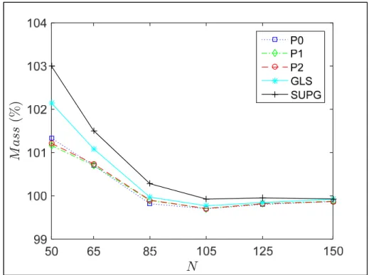
number of elements for each mesh. ...62 Table 4.1: Time-reversed vortex flow. Percentage of the disk mass loss
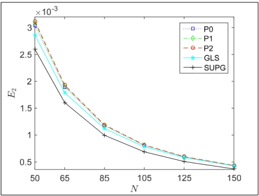
at for . ...90 Table 4.2: Time-reversed vortex flow. Error norms and at . ...90 Table 4.3: Rigid body rotation of Zalesak’s disk. Percentage of
the disk mass loss at for . ...92 Table 4.4: Rigid body rotation of Zalesak’s disk.
Error norms and at . ...92 Table 4.5: Rising bubble. Centre of mass and rise velocity . ...105
t T= t T= T =8 1 E E2 t T= t T= T =6.28 1 E E2 t T= c y vc
LIST OF FIGURES
Page
Figure 2.1: Two-phase domain. ...15
Figure 2.2: Interpolation of the interface. ...18
Figure 2.3: Example of 2-dimensional domain. ...19
Figure 2.4: Configuration of the domain for the fast marching method (FMM). ...20
Figure 2.5: Arborescent structure of a binary tree. ...23
Figure 2.6: Exact level sets solution (a), disturbed level sets (b), level sets after geometric reinitialisation (c), and level sets after the FMM (d) for the 64×64 mesh ...27
Figure 2.7: Error norm versus ...28
Figure 2.8: Error norm versus ...29
Figure 2.9: Error norm versus ...29
Figure 2.10: Error norm versus ...30
Figure 2.11: Error norm versus ...31
Figure 2.12: Error norm versus ...31
Figure 2.13: Error norm versus ...32
Figure 2.14: Error norm versus ...32
Figure 2.15: Time-reversed vortex flow. Interface positions at and with the 125×125 mesh using the Eikonal reinitialisation. Closer view of interface positions at (f). ...34
Figure 2.16: Time-reversed vortex flow. Percentage of disk area versus time using the Eikonal reinitialisation. ...35
Figure 3.1: Exact level sets solution (a), disturbed level sets (b), level sets after the geometric reinitialisation (c) ...50
1 E N 2 E N 3 E N 4 E N 1 E l 2 E l 3 E l 4 E l 0( ), / 4( ), / 2( ), 3 / 4 ( )and ( ) t= a T b T c T d T e T
( )
% MassFigure 3.2: Error norm versus ...51 Figure 3.3: Error norm versus ...52 Figure 3.4: Error norm versus ...52 Figure 3.5: Time-reversed vortex flow. Mesh of 65×65 and
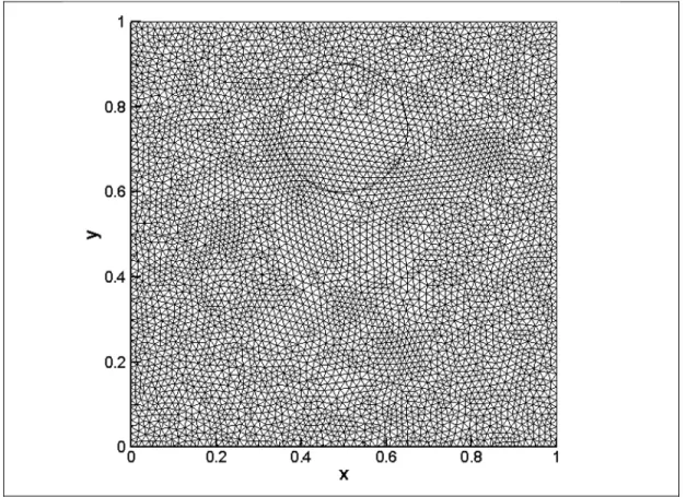
initial interface at t = 0 ...54 Figure 3.6: Time-reversed vortex flow. Percentage of
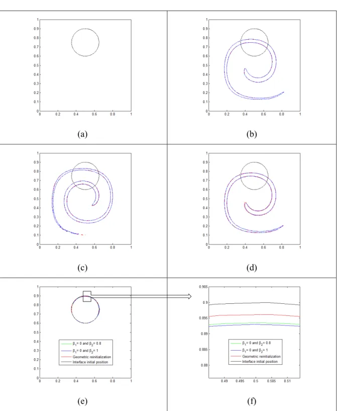
the disk mass at for . ...55 Figure 3.7: Time-reversed vortex flow. Interface positions at
and
with the 85×85 mesh. Closer view of interface positions at (f). ...56 Figure 3.8: Time-reversed vortex flow. Percentage of the disk area
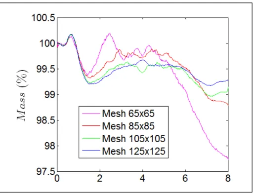
versus time for case 1: and . ...57 Figure 3.9: Time-reversed vortex flow. Percentage of the disk area
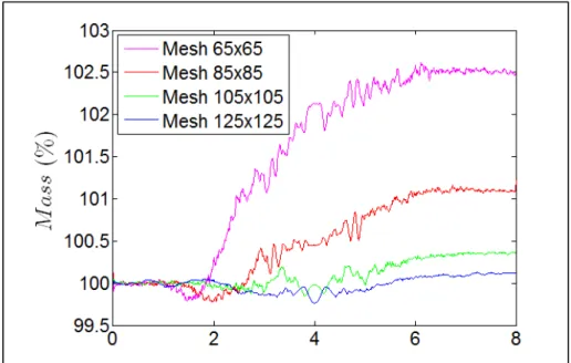
versus time for case 2: and . ...58 Figure 3.10: Time-reversed vortex flow. Percentage of the disk area
versus time for case 3: and
with geometric reinitialisation at each time step. ...58 Figure 3.11: Time-reversed vortex flow. Percentage of the disk area
versus ...60 Figure 3.12: Time-reversed vortex flow. Error norm versus ...61 Figure 3.13: Rigid body rotation of Zalesak’s disk. Coarse mesh and
initial interface at t = 0. ...62 Figure 3.14: Rigid body rotation of Zalesak’s disk. Percentage of
the disk mass at . ...63 Figure 3.15: Rigid body rotation of Zalesak’s disk. Interface positions at
for the stabilized formulation and for with the 85×85 mesh (a). Closer view of interface positions at (b). ...64 Figure 3.16: Rigid body rotation of Zalesak’s disk. Percentage of the disk area
at for . ...65 1 E N 2 E N 3 E N t T= T =8 0( ), / 4( ), / 2( ), 3 / 4 ( )and ( ) t= a T b T c T d T e T
( )
% Mass β1 =1 β2 =0( )
% Mass β1=0 β2 =1( )
% Mass β1 =0 β2 =0( )
% Mass N 2 E N t T= 0, / 4, / 2, 3 / 4, and t= T T T T T( )
% Mass t T= T =6.28Figure 3.17: Dam break. Mesh and initial interface at t = 0 s. ...69 Figure 3.18: Dam break interface position at t = 0.23s for
the geometric reinitialisation and the P1 projection. ...70
Figure 3.19: Dam break interface position at t = 0.5 s for
the geometric reinitialisation and the P1 projection. ...71
Figure 3.20: Dam break interface position at t = 0.75s for
the geometric reinitialisation and the P1 projection. ...71
Figure 3.21: Dam break interface position at t = 0.7s for
the P1, P2 and P3 projections. ...72
Figure 3.22: Dam break interface position at t = 0.8s for
the P1, P2 and P3 projections. ...72
Figure 3.23: Dam break interface position at t = 0.9s for
the P1, P2 and P3 projections. ...73
Figure 3.24: Dam break interface position at t = 1.0s for
the P1, P2 and P3 projections. ...73
Figure 3.25: Dam break. Evolution of the lower subdomain . ...74 Figure 3.26: Dam break. Position of the water column front on the bed (a)
and height of the water column on the left boundary (b). ...74 Figure 4.1: Time-reversed vortex flow. Interface positions at
.
Closer view of the interface at ...88 Figure 4.2: Time-reversed vortex flow. Percentage of disk area
versus time. ...89 Figure 4.3: Rigid body rotation of Zalesak’s disk. Interface positions at
.
Closer view of the interface at (b) ...91 Figure 4.4: Rigid body rotation of Zalesak’s disk.
Evolution history of the . ...91 Figure 4.5: Sloshing flow in a cavity. Initial interface at t = 0 s ...93
( )
% Mass 0( ), / 4( ), / 2( ), 3 / 4 ( )and ( ) t= a T b T c T d T e ( ) T f( )
% Mass 0, / 4, / 2, 3 / 4and (a) t= T T T T T( )
% MassFigure 4.6: Sloshing flow in a cavity. Interface positions at
...94 Figure 4.7: Sloshing flow in a cavity. The mass loss of the lower subdomain. ...95 Figure 4.8: Sloshing flow in a cavity, with the pressure at
. ...96 Figure 4.9: Dam-break. Mesh and initial interface at t = 0 s. ...98 Figure 4.10: Dam-break. Interface positions at
. ...99 Figure 4.11: Dam-break. The mass loss of the lower subdomain. ...100 Figure 4.12: Dam-break. Position of the water column front on the bed (a)
and the height of the water column on the left boundary (b). ...100 Figure 4.13: Dam break. The pressure at
. ...101 Figure 4.14: Rising bubble. Centre of mass ordinate (a), rise velocity (b),
(c), and theinterface at t = 3s (d). ...104 Figure 4.15: Dam break over an obstacle. Mesh and initial interface at t = 0 s. ...105 Figure 4.16: Dam break with an obstacle. Interface positions at
. ...106 Figure 4.17: Dam break with an obstacle. The mass loss of
the lower subdomain. ...107 Figure 4.18: Dam break with an obstacle. The pressure at
. ...108 Figure 4.19: Rayleigh-Taylor instability. Interface position at
with the mass conservation ...110 Figure 4.20: Rayleigh-Taylor instability. Velocity field,
velocity vector and interface position at
0 ( ), 0.5 ( ),1 ( ),1.5 ( ), 2 ( ), 2.5 ( )and 3 ( ) t= s a s b s c s d s e s f s g 0.5 ( ),1 ( ),1.5 ( ), 2 ( ), 2.5 ( )and 3 ( ) t= s a s b s c s d s e s f 0 ( ), 0.2 ( ), 0.4 ( ), 0.6 ( ), 0.8 ( )and1 ( ) t= s a s b s c s d s e s f 0.2 ( ), 0.4 ( ), 0.6 ( ), 0.8 ( )and1 ( ) t= s a s b s c s d s e c y vc (%) Mass 0 ( ), 0.2 ( ), 0.4 ( ), 0.6 ( ), 0.8 ( )and1 ( ) t= s a s b s c s d s e s f 0.2 ( ), 0.4 ( ), 0.6 ( ), 0.8 ( )and1 ( ) t= s a s b s c s d s e 0.25 ( ), 0.7 ( ),1.25 ( ),1.5 ( ),1.85 ( ), t= s a s b s c s d s e 2 ( ), 2.25 ( ), 2.5 ( ), 2.75 ( )and 3 ( )s f s g s h s i s j 0.25 ( ), 0.7 ( ),1.25 ( ),1.5 ( ),1.85 ( ), t= s a s b s c s d s e
with the mass conservation ...111 Figure 4.21: Rayleigh-Taylor instability. Pressure field and
interface position at
with the mass conservation ...112 Figure 4.22: Rayleigh-Taylor instability. The mass loss of
the lower subdomain. ...113 2 ( ), 2.25 ( ), 2.5 ( ), 2.75 ( )and 3 ( )s f s g s h s i s j
0.25 ( ),1 ( ),1.85 ( ), and 3 ( )
INTRODUCTION
Technological advances in recent years in the field of computer science for both hardware and software have contributed to the use of numerical simulations for the prediction of fluid flow. Numerical simulations can be combined with experimental methods to considerably reduce the time and cost of benchmark creation and the development and improvement costs of products. These benefits of numerical simulation software and new computer technologies on experimental methods have contributed to the development of new robust numerical methods in the field of “computational fluid dynamics” (CFD). Numerical simulations often provide accurate results more quickly and cheaply than experimental studies. The simulation of multiphase flows, which is a constituent of CFD, takes advantage of the computer technology benefits of both software and hardware by developing new numerical approaches to analyse these complex flows.
In physics and chemistry, the phase concept is used to specify the diverse states of a system. The phase concept or notion is also known by the term “state of matter”. There are three states of matter: gas, liquid and solid. A system consists of a single phase if it is entirely homogeneous, both physically and chemically. Otherwise, each of the various homogeneous parts that may be continuous or dispersed within each other can be called a phase.
A multiphase flow is the simultaneous flow of several phases. The two-phase flow is a special case of a multiphase flow where there are only two phases. Two-phase models can be classified according to the natures of the phases in the flow:
• gas-solid flow; • liquid-solid flow;
• liquid-liquid flow (immiscible liquids); and • gas-liquid flow.
0.1 Problem
Multiphase flows are present all around us, and there are many examples that we can find both in nature and in technical and industrial processes. For instance, for the flow of gas and liquid mixtures, we have studies of clouds, raindrops, liquid aerosol injection, inkjet printing, the free surface flow of a liquid (river or sea), moulding, liquid sloshing in a tank, air and water mixing through porous soil in geothermal wells, gas and oil mixtures in petroleum extraction, bubble column reactors, steam generators, turbines, electrohydraulic dam design and the hydrodynamics of ships. Studies of mixtures of immiscible liquids of importance include water and oil and pollutant transport after a spill of oil in the ocean.
Phase changes may also result in a transition from a liquid flow to a mixed gas and liquid flow and vice versa. This phenomenon is found in the boiling process of a liquid in a boiler, the liquefaction of saturated vapour exiting a turbine to form a mixture of water and saturated vapour, and the cavitation of a hydraulic pump. Cavitation is an important phenomenon that must be taken into account in the design of hydraulic components and hydraulic systems such as pumps and valves. Cavitation is induced by a pressure drop that is lower than the pressure of the saturated vapour. In the case of pump cavitation, gas bubbles are formed, leading to a loss of efficiency that influences the operation of the device. When there is cavitation in a hydraulic pump, the implosion of the bubbles can cause the tearing of the material on the blades of the pump and thereby drastically damage the pump.
Spraying liquid into fine droplets in the air is another application widely used in the food industry to clean food or to dry a fluid injected by atomisation in hot air to recover it in a solid form, for example, for the production of milk or powdered juice. Liquid spraying can also be found in the injectors that supply fuel to a combustion chamber.
This flow example list is not exhaustive, and we could add many other cases of multiphase flow and phase transition in nature and in industrial processes.
Numerical methods allow us to avoid experimental methods in the study of multiphase flows, which are often difficult to implement. The pressure, velocity and temperature measurements can be obtained by average or local measurements, but the measuring instruments often have
an impact on the fluid flow or require physical access to the field flow. In the case of multiphase flows, the discontinuity of properties between the phases can make the data measurement difficult. For these reasons, computer simulations are very popular currently for the study of multiphase flows. Numerical methods allow us to reproduce and analyse physical phenomena to have a better understanding of them. Numerical simulations let us extrapolate a simulation to other cases after their validation using experimental data. Research on two-phase flows involves many difficulties because of the technical complexity of the phenomena being modelled and the poor resolution of these models using numerical methods.
The modelling of multiphase flow requires not only to solving the Navier-Stokes equations but also finding the position of the interface between the phases. This is not an easy task, not only because of the complexity of the discontinuity of the physical properties at the interface between the phases, resulting in the nonlinearity of the Navier-Stokes equations governing the flow field but also the difficulty of keeping the mass (area or volume) of each phase of the domain constant over time during the numerical simulation. Furthermore, in the case where the surface tension between the phases is taken into account, the level of complexity needed to solve the fluid flow equations in diphasic flow increases considerably. In two-phase flow, there is an interface between the two phases that distinctly separates the two phases into two subdomains. The difference between the fluid properties across the interface presents major difficulties in the resolution of this type of problem because it induces a velocity gradient jump (continuity of shear) and / or a jump in pressure (surface tension) on both sides of the interface. In this work, we use the finite element method for the finite discretisation of the problem. The solution of the equations in 2D is done by the eXtended Finite Element Method (XFEM) with the Crank-Nicholson scheme for time discretisation and a quadratic space discretisation by a grid of triangular elements. Because of the high Reynolds number in some cases, the Galerkin formulation becomes unstable. Stabilisation techniques such as Streamline-Upwind Petrov-Galerkin (SUPG) or Petrov-Galerkin/Least-Squares (GLS) must be applied in this case to obtain a solution without oscillations.
The numerical solution of problems of immiscible phase flow can be classified into two basic approaches known as Eulerian (“interface capturing”) and Lagrangian (“interface tracking”).
In the Eulerian method, the properties are observed at a fixed point in space, while in the Lagrangian approach, the particles are tracked.
For example, an experimental Eulerian approach would entail taking, at a fixed point in a pipe, the measurement of the velocity with an anemometer or the measurement of the temperature with a thermocouple, giving the variation of the velocity or the temperature, respectively, at that fixed location over time. Among the Eulerian numerical methods (“interface capturing”) that describe the interface implicitly by an auxiliary field defined in the entire domain, we can cite the level set method and the Volume of Fluid method (VOF). In contrast, in the case of a Lagrangian approach (“interface tracking”), the particles are followed. In this case, the velocity or the temperature of a particle is a function of time depending on its path. By analogy, numerical methods of monitoring the interface (“interface tracking”) take into account the displacement of the interface by aligning elements that are at the interface during the simulation.
In two-phase flow, there is a discontinuity of the fluid properties through the interface. In the case of the interface-tracking method, this physical property discontinuity does not require additional treatment when the edges of all mesh elements located at the interface position are perfectly aligned with the interface. Furthermore, the interface-capturing method requires special treatment of the discontinuities across the interface because of the jump in the properties along the interface. The standard function forms of the finite element method are not able to correctly reproduce a discontinuous solution. In general, to overcome this problem by using the method of standard finite elements, there are two possible solutions that could be applied to a small band around the interface: refine the mesh on a narrow band around the interface or smooth the physical property discontinuity at the interface. These two methods can be used separately or combined together. However, the mesh refinement approach and the smoothing of physical properties at the interface may induce diffusion effects that could spread from the interface to the entire domain. To avoid the re-meshing and the diffusion effect at the interface, a new method called XFEM, which is based on the enrichment of the approximation space by the Partition of Unity Method (PUM) to take into account the discontinuities of the elements crossed by the interface, was introduced. The approximation space of a classical finite
element is enriched locally by functions that allow the representation of an exact approximation of the discontinuities in the elements cut by the interface. However, the enrichment increases the number of degrees of freedom of the enriched elements and thereby the cost in computation time.
The discretisation of the governing equations is done in time with the semi-implicit Crank-Nicolson scheme, while the spatial discretisation is performed with quadratic triangular elements. The stabilisation method Streamline-Upwind Petrov-Galerkin (SUPG) is used to control the stability problems incurred with the Galerkin formulation method in the case of advection problems.
0.2 Goal (objective)
The main objective of our research is to develop a numerical method that allows obtaining accurate numerical solutions of two-phase flow problems. In detail, we are interested in developing stabilised finite element methods for the level set equation, a correction method for the interface to conserve mass, and a coupling technique of these methods with a Navier-Stokes solver based on the eXtended Finite Element Method (XFEM).
0.3 Announcement of the methodology
The level set method was chosen to follow the evolution of the interface. The level set method, which is a Eulerian method, has the advantage of supporting topological changes such as the coalescence and separation of a phase, in contrast to the Lagrangian methods where an arbitrary criterion must be set to detect the coalescence or separation of a phase. However, the level set method has a drawback that could be significant in some cases. Although the topological changes are intrinsic to the level set method, the level set function initialised as a signed distance can move away from the signed distance property through the simulation depending on the difficulty or the duration of the problem simulation. Currently, the classic method used to maintain the level function as a signed distance function is to reset the level set function
after a certain number of steps selected in an ad hoc manner. This reinitialisation can be done in the whole domain or on a narrow band that is located on both sides of the interface.
We will propose methods for stabilising the level set equation to improve the accuracy of the numerical solution so that the level set function remains as close as possible to a distance function and the proposed methods reduce the use of reinitialisation.
On the other hand, the fact that the level set method does not keep the mass constant has led us to apply a method of correcting the level set function to improve the mass conservation by moving the level set field; this correction involves a small displacement of the interface. The eXtended Finite Element Method (XFEM) is used instead of the conventional finite element method because of the discontinuity of the properties at the interface, which is best represented by shape functions with the enrichment of the space approximation by the eXtended Finite Element Method (XFEM).
The discretisation of the governing equations is done in time with the semi-implicit Crank-Nicolson scheme, while the spatial discretisation is performed with quadratic triangular elements. The stabilisation method Streamline-Upwind Petrov-Galerkin (SUPG) is used to control the stability problems incurred with the Galerkin formulation method in the case of advection problems. The strong coupling between the velocity and pressure fields and the level set field is achieved through an iterative algorithm for solving the Navier-Stokes equation followed by an algorithm for the resolution of the level set equation.
0.4 Plan of the thesis
The thesis has four chapters. The Introduction sets out the background work, describes the research objectives and sets out the thesis plan. CHAPTER 1 describes the state of the art in numerical methods for solving two-phase flows with the classical finite element method and the extended finite element method. This chapter shows the history, progress and usefulness of the research in the field of two-phase flows. We will highlight the areas of application of these methods, as well as the advantages and disadvantages of some techniques. CHAPTER 2 presents different methods for solving the transport problem of the level set function. The classical methods of solving the level set transport equation (section 2.1) and methods of
resetting the level set field are described (section 2.2). The various methods of resetting that are presented are the geometric method (2.2.1), the fast marching method (2.2.2) and the Eikonal reinitialisation method (2.2.3). CHAPTER 3 sets out the proposed stabilisation methods. CHAPTER 4 shows the resolution of the Navier-Stokes equations by the extended finite element method (XFEM) for the spatial discretisation and elaborates upon the mass conservation methods (section 0). The Conclusions succinctly summarise the results of the research and its lessons and outlines proposals and prospects for future research.
CHAPTER 1
LITERATURE REVIEW
1.1 The finite element method
The finite element first appeared in the 1950s in solid mechanics. The use of the finite element method is motivated by the need to solve problems that conventional methods such as strength of materials or machine components cannot resolve because of the complexity of the geometry or the structure. The finite element method was first applied to fluid mechanics in the 1970s. This delay in the use of the finite element method between solid mechanics problems and fluid mechanics problems is the result of, first, the strong coupling between the velocity and pressure and, second, the presence of a convective term in the Navier-Stokes equations, which implies a non-linearity. Furthermore, if the Reynolds number is very high, we could have turbulence phenomena. Among the early work on finite elements, we can include the work of Zienkiewicz and Cheung (Zienkiewicz et Cheung, 1965) in 1965, which presents the finite element method applied to the resolution of a quasi-harmonic partial derivative equation that one finds in conduction heat transfer problems and torsion of prismatic cross-section problems. In 1982, an algorithm based on the method of characteristics was proposed by Pironneau (Pironneau, 1982) to solve the transport-diffusion equation (convection-diffusion) and the Navier-Stokes equations, with a spatial discretisation made using Taylor-Hood elements. A new Streamline Upwind/Petrov-Galerkin (SUPG) formulation, which consists of adding diffusion or viscosity that acts only in the direction of the flow, was proposed (Brooks et Hughes, 1982). The SUPG method is more robust than the Galerkin method. A method called Galerkin/Least-Squares (GLS), which consists of adding the least squares form of the residual to the Galerkin method (Hughes, Franca et Hulbert, 1989), was presented, and it improves the stability while preserving the accuracy of the solution. Hughes et al. (Hughes, Franca et Balestra, 1986) presented a new Petrov-Galerkin formulation to solve the Stokes problem by introducing a stabilisation that avoids the use of Taylor-Hood mixed interpolations. This formulation provides a stable and convergent solution using a C0 approximation of the same order for the
“Discontinuous Galerkin Method” (DGM) formulations were proposed to solve diffusion problems (Oden, Babuŝka et Baumann, 1998) and convection-diffusion problems (Baumann et Oden, 1999). This hp-discontinuous finite element method is conservative, the order of approximation of the elements is adjusted by an element and the stability of the method does not require the insertion of an artificial diffusion term.
1.2 Interface problem solving methods
The numerical methods that allow solving the interface transport problem are generally classified into different approaches that are classified as Eulerian methods, Lagrangian methods and Eulerian-Lagrangian methods. The Eulerian methods include the “front-tracking” methods and the “front-capturing” methods. “Front-tracking” is based on markers and can be divided into two groups: tracking” and “surface-tracking” methods. In the “volume-tracking” methods such as “marker and cell method” (MAC), markers are distributed in all phases of the domain, while with the “surface-tracking” methods, markers are distributed only on the interface. During the simulation, the markers can gather in certain areas, resulting in the need for the redistribution of markers in the domain for the “volume-tracking” methods or on the interface for the “surface-tracking” methods to preserve the precision of the numerical results. The MAC method, which consists of distributing the markers in the domain, was applied to dam break problems (Harlow et Welch, 1965) . The “surface-tracking” methods are generally more accurate than the “volume-tracking” methods to return the interface position. “Surface tracking” methods have been developed by Glimm et al. to simulate shock waves in compressible flows (Glimm, 1982; Glimm et McBryan, 1985), and more recently, Unverdi and Tryggvason developed techniques to solve the Navier-Stokes equations when they are applied to the case of bubbles with a surface tension effect (Unverdi et Tryggvason, 1992). In the Lagrangian approach, the mesh is entirely or partially mobile and is updated at each time step. Lagrangian methods offer accurate solutions, but they are difficult to implement in 3D, in particular in the case of complex deformations of the interface. In the Lagrangian-Eulerian methods, such as the “Arbitrary Lagrangian-Eulerian formulation” (ALE) (Hu, Patankar et Zhu, 2001), the nodes of the mesh can be moved with the fluid according to the Lagrangian
method or can be held stationary according to the Eulerian method. Therefore, some mesh nodes can be moved from an arbitrarily specified criterion to provide a continuous rezoning functionality. Because of this freedom in the movement of the mesh in the ALE formulation, some cases of larger distortions within the domain can be treated, whereas a purely Lagrangian method or purely Eulerian method would not provide as much precision in the results.
The methods of the “front-capturing” are commonly used to study two-phase flow because they represent natural topological changes without additional ad hoc parameter settings. The most common “front-capturing” techniques are the Volume Of Fluid method (VOF) (Hirt et Nichols, 1981; Noh et Woodward, 1976; Youngs, 1982) and the level set method (Osher et Sethian, 1988). These last two methods are based on solving a scalar transport equation. The scalar transported by the VOF method and the level set method are the volume fraction and the level set function, respectively. Among the methods used for VOF, we can cite the method of “Simple Line Interface Calculation” (SLIC) (Noh et Woodward, 1976) and the method of “Piece Linear Interface Calculation” (PLIC) (Rider et Kothe, 1998), which are techniques used to find the position of the interface in the VOF method where the unknown variable is the ratio of each phase in a cell or element. In the level set method, introduced by Osher and Sethian (Osher et Sethian, 1988), the transported scalar is defined as a continuous function corresponding to the signed distance from the interface. Because of numerical errors that occur during the resolution of the level set transport equation, several reinitialisation processes have been suggested to allow the level set function to keep its signed distance property (Adalsteinsson et Sethian, 1999; Chunming et al., 2010; Gross et Reusken, 2011; Hysing et Turek, 2005; Olsson et Kreiss, 2005; Olsson, Kreiss et Zahedi, 2007; Osher et Fedkiw, 2003; Qian, Zhang et Zhao, 2007; Sethian, 1996; Sethian, 1998; So, Hu et Adams, 2011; Sussman, Smereka et Osher, 1994; Zhao, 2005). The main difficulty when re-distancing the level set function or using the approach of the mass conservation is that these methods can slightly move the position of the interface according to their frequency of use (Gomes et Faugeras, 2000). In our proposed technique (Touré et Soulaïmani, 2012; 2016), we combine the level set function transport equation and the reinitialisation equation in one variational formulation. However, the level set method can cause quite significant mass loss in some cases. There are many ways to overcome this weakness, such as
- The application of a mass conservation method after the reinitialisation of the level set function;
- The coupling of the level set method with the VOF method that conserves the mass in an intrinsic way; or
- The global refinement of the mesh or the local refinement of the mesh in the vicinity of the interface.
Several studies were conducted to enforce the mass property conservation in the context of the application of the level set method (Ausas, Dari et Buscaglia, 2011; Desjardins, Moureau et Pitsch, 2008; Di Pietro, Lo Forte et Parolini, 2006; Doyeux et al., 2013; Kees et al., 2011; Kuzmin, 2014; Laadhari, Saramito et Misbah, 2010; Le Chenadec et Pitsch, 2013; Olsson et Kreiss, 2005; Olsson, Kreiss et Zahedi, 2007; Owkes et Desjardins, 2013; Smolianski, 2001; Sussman, 2003; Sussman et Puckett, 2000; van der Pijl et al., 2005; Wang, Simakhina et Sussman, 2012). In our two-phase flow studies, only one of the two phases is forced to preserve its global mass (Gross et Reusken, 2011; Smolianski, 2001).
1.3 The methods of solving the Navier-Stokes equations by the eXtended Finite Element Method (XFEM)
The Navier-Stokes equations for two-phase flow can be solved by the “eXtended Finite Element Method” (XFEM) (Chessa et Belytschko, 2003a) or the ghost fluid method (Ménard, Tanguy et Berlemont, 2007), which takes into account the discontinuities of the physical properties of elements cut by the interface. The XFEM is established based on the partition of unity method (Babuška et Melenk, 1997; Babuška, Caloz et Osborn, 1994; Melenk et Babuška, 1996), where the discontinuities of properties in the finite elements are treated through the enrichment of the shape functions by adding degrees of freedom.
We find the practical application of XFEM in fluid mechanics problems in many areas and past research (Chessa et Belytschko, 2003a; Chessa et Belytschko, 2003b; Fries, 2009; Fries et Belytschko, 2006; Groß et Reusken, 2007; Gross et Reusken, 2011; Reusken, 2008). Chessa and Belytschko proposed solving the Navier-Stokes equations for a two-phase flow with and without the effect of surface tension by the XFEM method using the “abs-enrichment”
formulation, which consists of introducing the absolute value of the level set function into the shape functions to reflect the jump in the velocity field at the interface (Chessa et Belytschko, 2003a; Chessa et Belytschko, 2003b). Gross and Reusken proposed the enrichment of the pressure approximation space using a Heaviside function (Groß et Reusken, 2007). Their XFEM method was applied to 3D two-phase flows with surface tension. An adaptive mesh and a mesh refinement at the interface are also presented. Fries and Belytschko (Fries et Belytschko, 2006) introduced the intrinsic XFEM, which is applied to two-phase flow (Fries, 2009). The intrinsic XFEM, unlike the extrinsic XFEM, does not require the addition of supplementary unknowns. Coppola-Owen and Codina (Coppola-Owen et Codina, 2005) introduced an enrichment function for discontinuous pressure gradients of two-phase flow, which are zero at the nodes of the cut elements whose gradient is constant on either side of the interface. Zlotnik and Díez (Zlotnik et Díez, 2009) generalised the “abs-enrichment” function according to Moës et al. (Moës et al., 2003) for multiphase flow problems by introducing a hierarchical collection of (n-1) level set functions for n phases in the domain. The approximation spaces of the velocity and the pressure are enriched for the numerical simulation of the Stokes problem. The coupling of the “abs-enrichment” method of Moës and the enrichment method using the Heaviside function were investigated for incompressible fluids (Legrain, Moës et Huerta, 2008).
Although the XFEM method ensures a better approximation than the standard finite element method for discontinuous solutions, we can face convergence problems with the iterative numerical methods. Indeed, XFEM may tend to poorly conditioned matrix systems, especially when the interface is very close to a node or when the ratio between the volumes of the two sides of the interface of the cut elements is very high (Fries et Belytschko, 2010). On the other hand, the “Generalised Finite Element Method” (GFEM) is a “Partition of Unity Method” (PUM), where the space of the Finite Element Method (FEM) is increased by using non-polynomial shape functions with compact support. Recently, Babuška and Banerjee presented a new method called the “Stable Generalised Finite Element Method” (Stable GFEM/XFEM) (Babuška et Banerjee, 2012). The Stable XFEM method was applied to two-phase flows (Sauerland et Fries, 2013). A preconditioner can be used so that the matrix systems are well-conditioned. Bechet et al. applied a preconditioner based on a local Cholesky decomposition
(Béchet et al., 2005), while Menk and Bordas (Menk et Bordas, 2011) used a preconditioner related to the domain decomposition procedure. Another method consists of moving the nodes of the cut elements in which the interface is very close to one of their nodes to obtain a proportional volume ratio of the two sides of the interface of the cut elements that can greatly improve the conditioning of the matrix system (Choi, 2011).
1.4 The coupling between the Navier-Stokes and the level set equation
The coupling between the velocity/pressure field and the level set field can be done by
- a resolution of a unique matrix system including the Navier-Stokes equations and the level set transport equation;
- a weak coupling of the Navier-Stokes equations whose unknowns are the couple of velocity and pressure obtained from the previous level set solution step and then doing an update of the level set function; or
- a strong coupling by performing iterations of the weak coupling method until the equilibrium (or balance) of the velocity, pressure and level set fields is achieved.
The weak coupling can lead to non-physical results, according to Akkerman et al. (Akkerman et al., 2011). The strong coupling is less expensive than the resolution of the Navier-Stokes equations and transports the level set function equation combined in a unique matrix system. Strong coupling was used in our case of a two-phase flow study.
CHAPTER 2
CLASSIC LEVEL SET METHODS
2.1 The level set method
The level set method was introduced in 1988 by Osher and Sethian (Osher et Sethian, 1988). The starting point of this method is the definition of a level set scalar function
φ
. The zero value of the level set function is the interface that is transported by the velocity field. The contours of the level set function initialized as a distance function may move away from the level set distance function due to the accumulation of numerical errors; hence, in classical reinitialisation methods the solution needs to be reset after a certain number of time steps. The moving interface Γ( )
t is defined as the zero-level for the scalar functionφ( )
x,t :( )
t{
x 3|φ
( )
x t, 0}
Γ = ∈R = . (2.1)
For example, in a two-phase flow, as illustrated in Figure 2.1, the entire domain Ω = Ω1Ω2 is divided into two subdomains Ω1 and Ω2 separated by the interface Γ
( )
t according to the sign of the level set function:( )
( )
( )
1 2 , 0 , 0 , 0 t if t if t if φ φ φ < ∈Ω = ∈Γ > ∈Ω x x x x x x . (2.2)Most often, the level set function is the signed distance function, which is defined by:
( )
( )
( )
1 2 , if , 0 if , if signed d t d t d t − ∈Ω = ∈Γ ∈Ω x x x x x x (2.3) with( )
, min(
)
d t Γ Γ ∀ ∈Γ = x − x x x (2.4)The signed distance function has the following useful property:
1
signed
d
∇ = (2.5)
which is an Eikonal equation. The level set function is initialized by the signed distance,
( )
, 0 dsigned( )
, 0φ x = x , and its evolution is governed by the transport equation:
( )
,( )
,( )
, 0 D t t t Dt t φ ∂φ φ = + ⋅∇ = ∂ x x u x (2.6) or 0 F t φ φ ∂ + ∇ = ∂ (2.7) where F un φ φ ⋅∇ = = ∇ uis the velocity component in the normal direction to the isocontours of
φ
. Equation (2.6) or (2.7) is called the level set equation (Osher et Sethian, 1988).The unit (outward) normal vector is determined by ˆ φ
φ
∇ =
∇
n and the mean curvature
κ
isdefined as the divergence of ˆn so that κ ˆ φ
φ
∇ = ∇⋅ = ∇⋅
∇
n . Since the interface is moving with a conservative flow field, the total area is conserved for both phases:
( )
( )
1 2 0 if , 0 0 if , 0 D t Dt D t Dt φ φ Ω = < Ω = > x x (2.8)2.2 The reinitialisation methods
The numerical discretisation of the level set transport equation (2.6) does not necessarily conserve the signed distance function property (2.5). However, this latter property is essential to maintain good accuracy in the calculation of geometric quantities related to the interface and in the determination of the position of the interface. In the case of two-phase flows where the velocity fields can significantly stretch or tighten the level set, it is necessary to apply a constraint on the evolution of
φ
in such a way that ∇φ
signed remains close to 1 withoutsignificantly moving the interface Γ .
2.2.1 The geometric reinitialisation method
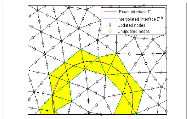
The geometric reinitialisation is a “brute force search algorithm” and is described as follows: The elements crossed by the interface Γ are first found (Figure 2.2). We suppose that any element crossed by the interface has only two points with a zero level such that each point belongs to a different edge. Next, a piecewise linear approximation Γh of the interface is computed by joining these zero-level points, as illustrated by the blue segments in Figure 2.2. The nodes belonging to the crossed elements (cut elements) are labelled as “un-updated nodes” because their level set values are unchanged from the results computed by solving (2.6). For the other nodes (labelled as updated nodes), the level set values are corrected and set to the recomputed signed distance to the interface Γh. When this reinitialisation algorithm is used at
each time step, it is expected to produce accurate results that can serve as references for comparison. Therefore, we do not expect or claim that the proposed stabilisation algorithms will perform better, but rather will produce acceptable results with simplified implementation.
Figure 2.2: Interpolation of the interface.
2.2.2 The fast marching method (“The boundary value formulation”)
The fast marching method (FMM) (Sethian, 1996; Sethian, 1998) is a popular technique for reinitialisation and describes an interface that only expands or only contracts. It is expressed with the boundary value formulation,
1
T F
∇ = (2.9)
where T is the arrival time function and F x
( )
is the normal velocity un at the interface. This equation is an Eikonal equation and applies only when the front moves in one direction. The arrival function T T= x( )
gives the duration that the front starting from the interface takes to reach the point x=( )
x y, . This arrival function is the basic function of the fast marching method (FMM) (Sethian, 1996; Sethian, 1998). Furthermore, we have the relation( ) ( )
,t T tthen we must use the Eikonal reinitialisation method (also known as the “Initial Value Formulation”) (see Section 2.2.3).
The proposed upwind scheme (Sethian, 1998) for the 3D spatial discretisation is
(
)
(
)
(
)
1 2 2 2 2 max , , 0 1 max , , 0 max , , 0 x x ijk ijk y y ijk ijk ijk z z ijk ijk D T D T D T D T F D T D T − + − + − + − + − + = − (2.10)where D is the difference operator such as for example the forward difference operator is
( , ) ( , ) x x x t x t D x α α α + = + Δ −
Δ , the backward difference operator
( , ) ( , ) x x t x x t D x α α α − = − − Δ Δ and the centred difference operator is 0 ( , ) ( , )
2 x x x t x x t D x α α α= + Δ − − Δ Δ .
In 2D, as illustrated in Figure 2.3, on a structured Cartesian grid of size element h= Δ Δ
(
x y,)
, we obtain the following spatial discretisation:( )
(
)
2 , 1, 1, , 2 , , 1 , 1 , 2 max , ,0 1 max , ,0 , i j i j i j i j i j i j i j i j T T T T x x T T T y y F x y T − + − + − − − + Δ Δ − − − = Δ Δ (2.11)For this boundary value formulation, the normal velocity should be strictly positive (F >0) or strictly negative (F<0), regardless of the time. The FMM is useful when the interface can only move in one direction, while in the initial value formulation (see section 2.2.3), there is no limitation on the sign of the normal velocity F of the interface.
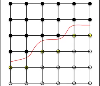
The goal of the method is to propagate a front from the interface along the outward normal direction by progressively computing the distance from the interface to the nodes of the mesh that are reached by the propagated front, as illustrated in Figure 2.4, where the front moves toward the southeast direction.
Legend 1 Interface Known or frozen nodes Accepted or narrow band nodes Not accepted or far away nodes
Figure 2.4: Configuration of the domain for the fast marching method (FMM).
The initialisation of the distance of the nodes is performed using, as a reference, the nodes of the elements that are cut or adjacent to the interface. The aim of the method is to determine the distance between the interface and the nodes that are adjacent to the nodes whose distance to the interface is already known. The front is moving along the outward normal direction with a normal velocity F.When the front crosses a new node of the mesh, it becomes part of the known nodes (or frozen nodes) set, and its signed distance will be computed. The distances of the closest nodes to the interface (accepted or narrow band nodes) that are on the opposite side of the known nodes are computed one after the other. The distances of the other nodes (not accepted or far away nodes) are temporary. They must be recalculated using the newly admitted nodes and their distance. The fast marching method (FMM) must perform quickly and recursively the following process.
Algorithm or procedure of reinitialisation by the fast marching method (FMM)
Initialisation step
1. Initialise the front by detecting the points on the interface. The nodes on the interface and upstream of the interface are labelled “Known nodes” (or “Frozen nodes”) , and their value of T is assigned to them. The nodes immediately adjacent to the “Known nodes” are labelled “Accepted nodes” (or “Narrow band nodes”) . The value of T
of the “Accepted nodes” (or “Narrow band nodes”) is initialised by solving equation (2.11). All other nodes are labelled “Not accepted nodes” (or “Far away nodes”) , and they are on the downstream side of the “Accepted nodes” (or “Narrow band nodes”). The value T of the “Not accepted nodes” (or “Far away nodes”) is initialised numerically to +∞.
Iterative loop stage 2. Start of the loop.
Determine the node p (“Trial node”) of coordinates xp such that the distance
( )
p min(
( )
)
Narrow Band T T ∈ =xx x and then add the node to the Known (or Frozen) nodes and remove it from the “Accepted nodes” (or “Narrow band nodes”).
3. Label all nodes that are adjacent to the node p to the “Accepted nodes” (or “Narrow band nodes”) if they do not belong to the “Known nodes” (or “Frozen nodes”). If some of the neighbouring nodes that meet these last criteria are part of the “Not accepted nodes” (or “Far away nodes”), add them to “Trial nodes” and remove them from “Not accepted nodes” (or “Far away nodes”).
4. Recalculate value T for all the neighbours of the node p by solving equation (2.11). 5. Return to the start of the loop at step 2.
End of the loop
Sorting and efficiency of the algorithm
To speed up step 2 of the search algorithm, we use a complete binary tree including the nodes of the “Accepted nodes” (or “Narrow band nodes”) and their temporary distance as shown in Figure 2.5 and
Table 2.1, where k is the position of the node and T is the nodal value.
The node p (“Trial node”) that has the smallest distance is the root of the binary tree. When the node is removed from the tree, the other nodes are moved to the top of the tree to form a new tree.
Figure 2.5: Arborescent structure of a binary tree.
Table 2.1: Structure of a binary tree in an array
Property of the binary tree implemented in an array
The access time to a node is O(1). A balanced insertion or removal of a node in the tree spends
(log )
O N in time. The fast marching method calculates the distance of N nodes in
( log )
O N N in the worst case. For example, in a two- or three-dimensional mesh of n nodes in each direction, the total number of operations is n2logn or n3logn, respectively.
2.2.3 The Eikonal reinitialisation method (“The initial value formulation”)
The transport equation of the level set (2.6) is solved for a number of time steps using temporal discretisation and spatial discretisation. If the level set function is no longer a distance function because of error accumulation, a correction procedure is usually adopted, such as solving a
reinitialisation (or redistancing) equation as proposed by Sussman, Smereka and Osher (Sussman, Smereka et Osher, 1994),
( )
0(
1)
0 S t ϕ ϕ ϕ ∂ + ∇ − = ∂ (2.12)where τ is a pseudo-time. Equation (2.12) is solved with the initial condition
( )
,0 0( )
,tϕ
x = =ϕ φ
x . At convergence, a corrected level setϕ
( )
x,t is obtained, satisfying1 0
ϕ
∇ − . The sign function S
( )
ϕ
0 is defined by( )
0 00 0 1 0 0 0 1 0 si S si si ϕ ϕ ϕ ϕ > = = − < (2.13)where S
( )
ϕ
0 can also be smoothed to( )
00 2 2
0
S ϕ
ϕ ε
ϕ =
+ , as proposed by Sussman et al.
(Sussman, Smereka et Osher, 1994), or
( )
00 2 2 2 0 0 S ε ϕ ϕ ϕ ϕ =
+ ∇ , as suggested by Peng et al. (Peng et al., 1999).
The accuracy of this method depends on the time interval between the two reinitialisation steps. The time after which the level set solution is reinitialised should be chosen in a suitable manner. The reinitialisation process may move the zero level set contours from their initial position (Gomes et Faugeras, 2000). However, when the level set function
φ
( )
x,t is too far from the signed distance functiondsigned, the reinitialisation process may fail. It is correctly stated inGross-Reusken (Gross et Reusken, 2011) that ‘using this technique, one faces the following difficulties. Firstly, the method contains control parameters τ and ε , and there are no good practical criteria on how to select these. Secondly, the partial differential equation (2.12) is nonlinear and hyperbolic; accurate discretisation of this type of partial differential equation is rather difficult’, and the stability and convergence depend on those parameters involved in the stabilised formulation.
In fact, we have implemented a finite element discretisation of the multiscale variational formulation proposed by Akkerman et al. (Akkerman et al., 2011; Kees et al., 2011), and we faced the same difficulties as those reported in Gross-Reusken (Gross et Reusken, 2011), namely, that the stability and convergence depend on the control parameters t and ε and the parameters involved in the stabilised formulation. Akkerman et al. (Akkerman et al., 2011) proposed the formulation
( )
( )
0 d h h d h h x d h h d h h x x d S d t S d t ε φ ε φ η φ φ φ τ η φ φ Ω Ω ∂ + ⋅∇ − Ω ∂ ∂ + ⋅∇ + ⋅∇ − Ω = ∂ a a a (2.14) where( )
h x dh h x d Sε φ φ φ ∇ = ∇ a and Sε( )
φ
=2Hε( )
φ
−1 (2.15)Hε is the regularised Heaviside function.
Akkerman et al. suggested to add a penalty term to equation (2.14) to maintain the interface at its position during the reinitialisation (Akkerman et al., 2011). The proposed penalty term is
( )(
)
' h h h h penalHε d d η λ φ φ φ Ω +
− Ω (2.16)where λpenal is a constant parameter.
The numerical tests
The following numerical tests were carried out to compare the accuracies of the proposed methods. First, in section 2.2.4, a numerical test was performed to evaluate the accuracy of the level set geometric reinitialisation and the fast marching method, described in section 2.2.1 and section 2.2.2, respectively, using disturbed level sets of a rectangular interface. In section 2.2.5, a test is performed to show the performance of the Eikonal reinitialisation previously presented in section 2.2.3. To analyse the solution accuracy, the following norms are defined:
( ) ( )
1 Ω ,0 , E =
φ x −φ xT dΩ (2.17)( ) ( )
(
)
2 2 Ω ,0 , E =
φ x −φ x T dΩ (2.18)( ) ( )
(
)
( )
2 3 2 ,0 , , 0 T d E d φ φ φ Ω Ω − Ω = Ω
x x x (2.19)( )
(
2)
4 , 1 E φ T d Ω =
∇ x − Ω (2.20)where
φ
( )
x,0 is the finite element interpolation of the exact solution at the initial time. Furthermore, to assess the mass (or area) conservation of a phase, the following percentage is defined as area( ) (%) 1 00 area( 0) t Mass t = = (2.21)2.2.4 The comparison of reinitialisation methods by the geometric method and the fast marching method
The interface Γ is defined as a rectangle. The nodal level set values are then obtained by computing the signed distance to the rectangular interface. The disturbed level set function is found by adding to the exact level set function a perturbing term, sin sin(20 )
20 2 r d r π θ ,
where r=1, d r= − x2+y2 and tan 1 y x θ = −
.
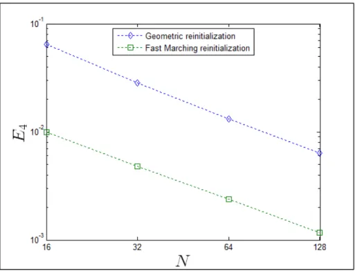
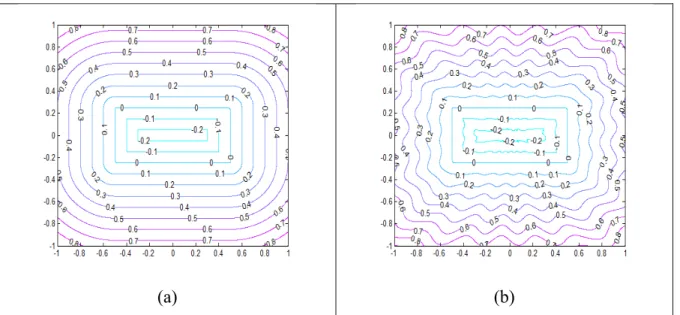
The computational domain is a unit square. The grid convergence study is performed for the structured meshes (N N× ) 16×16, 32×32, 64×64, and 128×128. The spatial discretisation is obtained with quadratic triangular elements. Figures 2.6 (a-d) show the level sets for the 64×64 mesh: for the exact level sets solution, the disturbed level sets, the level sets after the geometric reinitialisation is applied to the disturbed level sets, and the level sets after the fast marching method is applied to the disturbed level sets. The error norms of the reinitialisation method are shown in Figure 2.7 to Figure 2.10. The mass error is approximately ± ×2.5 10−12 for the
different meshes.
(a) (b)
Figure 2.6: Exact level sets solution (a), disturbed level sets (b), level sets after geometric reinitialisation (c),
Figure 2.6 continuation
(c) (d)
Figure 2.7: Error norm versus
-0.2 -0.2 -0.1 -0.1 -0 .1 0 0 0 0 0 0.1 0.1 0. 1 0.1 0.1 0.2 0.2 0.2 0.2 0.2 0.2 0.3 0.3 0. 3 0.3 0.3 0. 3 0.3 0.4 0.4 0.4 0.4 0.4 0.4 0. 4 0.4 0.5 0.5 0.5 0.5 0.5 0.5 0.5 0.5 0.6 0.6 0.6 0.6 0.6 0.6 0.6 0.6 0.7 0.7 0.7 0.7 0.7 0.7 0.8 0.8 0.8 0.8 -1 -0.8 -0.6 -0.4 -0.2 0 0.2 0.4 0.6 0.8 1 -1 -0.8 -0.6 -0.4 -0.2 0 0.2 0.4 0.6 0.8 1 1 E N
Figure 2.8: Error norm versus
Figure 2.9: Error norm versus 2
E N
3