A Simple Test of Learning Theory

Texte intégral

(1)2006s-30. A Simple Test of Learning Theory Jim Engle-Warnick, Ed Hopkins. Série Scientifique Scientific Series. Montréal December 2006. © 2006 Jim Engle-Warnick, Ed Hopkins. Tous droits réservés. All rights reserved. Reproduction partielle permise avec citation du document source, incluant la notice ©. Short sections may be quoted without explicit permission, if full credit, including © notice, is given to the source..

(2) CIRANO Le CIRANO est un organisme sans but lucratif constitué en vertu de la Loi des compagnies du Québec. Le financement de son infrastructure et de ses activités de recherche provient des cotisations de ses organisations-membres, d’une subvention d’infrastructure du Ministère du Développement économique et régional et de la Recherche, de même que des subventions et mandats obtenus par ses équipes de recherche. CIRANO is a private non-profit organization incorporated under the Québec Companies Act. Its infrastructure and research activities are funded through fees paid by member organizations, an infrastructure grant from the Ministère du Développement économique et régional et de la Recherche, and grants and research mandates obtained by its research teams. Les partenaires du CIRANO Partenaire majeur Ministère du Développement économique, de l’Innovation et de l’Exportation Partenaires corporatifs Alcan inc. Banque de développement du Canada Banque du Canada Banque Laurentienne du Canada Banque Nationale du Canada Banque Royale du Canada Banque Scotia Bell Canada BMO Groupe financier Bourse de Montréal Caisse de dépôt et placement du Québec DMR Conseil Fédération des caisses Desjardins du Québec Gaz de France Gaz Métro Hydro-Québec Industrie Canada Investissements PSP Ministère des Finances du Québec Raymond Chabot Grant Thornton State Street Global Advisors Transat A.T. Ville de Montréal Partenaires universitaires École Polytechnique de Montréal HEC Montréal McGill University Université Concordia Université de Montréal Université de Sherbrooke Université du Québec Université du Québec à Montréal Université Laval Le CIRANO collabore avec de nombreux centres et chaires de recherche universitaires dont on peut consulter la liste sur son site web. Les cahiers de la série scientifique (CS) visent à rendre accessibles des résultats de recherche effectuée au CIRANO afin de susciter échanges et commentaires. Ces cahiers sont écrits dans le style des publications scientifiques. Les idées et les opinions émises sont sous l’unique responsabilité des auteurs et ne représentent pas nécessairement les positions du CIRANO ou de ses partenaires. This paper presents research carried out at CIRANO and aims at encouraging discussion and comment. The observations and viewpoints expressed are the sole responsibility of the authors. They do not necessarily represent positions of CIRANO or its partners.. ISSN 1198-8177. Partenaire financier.

(3) A Simple Test of Learning Theory * Jim Engle-Warnick †, Ed Hopkins‡ Résumé / Abstract Nous faisons le compte rendu d'expériences élaborées afin de tester la possibilité théorique, découverte par Shapley (1964), que dans certains jeux, l'apprentissage ne converge pas vers un équilibre, que ce soit en termes de fréquences marginales ou de jeu moyen. Les sujets ont joué à répétition en paires fixes à un de deux jeux 3 × 3, chaque jeu ayant un équilibre de Nash unique avec stratégies mixtes. On prévoit que l'équilibre du premier jeu soit stable après apprentissage, et le deuxième jeu instable, à condition que les gains soient suffisamment élevés. Pour chaque jeu, nous avons eu recours à deux différents traitements : un avec gains faibles et l’autre avec gains élevés. Nous avons constaté que dans tous les traitements, le jeu moyen est près de l'équilibre bien qu'il y ait présence de cycles importants dans les données. Mots clés : jeux, apprentissage, expériences, jeu fictif stochastique, équilibres à stratégie mixte. We report experiments designed to test the theoretical possibility, first discovered by Shapley (1964), that in some games learning fails to converge to any equilibrium, either in terms of marginal frequencies or of average play. Subjects played repeatedly in fixed pairings one of two 3 × 3 games, each having a unique Nash equilibrium in mixed strategies. The equilibrium of one game is predicted to be stable under learning, the other unstable, provided payoffs are sufficiently high. We ran each game in high and low payoff treatments. We find that, in all treatments, average play is close to equilibrium even though there are strong cycles present in the data. Keywords: games, learning, experiments, stochastic fictitious play, mixed strategy equilibria. Codes JEL : C72, C73, C92, D83.. *. We thank John Galbraith, Steffen Huck, Tatiana Kornienko and Martin Sefton for helpful discussions. We thank Sara Constantino and Julie Héroux for research assistance. We gratefully acknowledge financial support from the Economic and Social Research Council, UK, the Nuffield Foundation, and Nuffield College, University of Oxford, UK. We thank the Economics Department, Royal Holloway, University of London and the Centre for Interuniversity Research and Analysis on Organizations (CIRANO) and the Bell University Laboratory in Electronic Commerce and Experimental Economy for use of the experimental laboratory. Errors remain our own. † Department of Economics, 855 Sherbrooke St. West, McGill University, Montreal, Quebec, H3A 2T7, Canada, e-mail: jim.engle-warnick@mcgill.ca; tel.: (514) 398-1559; fax: (514) 398-4938. ‡ Corresponding author, E.Hopkins@ed.ac.uk, http://www.homepages.ed.ac.uk/hopkinse.

(4) 1. Introduction. Recent work on learning is marked by the integration of theory and experimental investigation. There has been significant recent success in explaining observed laboratory decision-making through the use of learning theories (for example, Camerer and Ho, 1999; Erev and Roth, 1998). This has spurred theorists to do new work that advances in our understanding of how learning models work. This field in surveyed in Fudenberg and Levine (1998). However, there have been fewer experiments designed explicitly to test learning theory’s predictions.1 In this paper, we examine one particularly striking implication of learning theory: there are games in which play should never converge. We investigate experimentally two games that possess a unique Nash equilibrium in mixed strategies. In one game, learning theory predicts convergence to the mixed strategy equilibrium. In the other game, theory predicts that the equilibrium is unstable. That is, if the learning model we consider, stochastic fictitious play, accurately predicts the behavior of experimental subjects, their play should never settle down but rather should continue to cycle. We ran two treatments for both games, one with high and one with low monetary payoffs. Theory suggests that higher payoffs should increase divergence in the unstable game, but make play closer to equilibrium in the stable game. Our experiments reveal limited support for these hypotheses. In all treatments, average play seems to converge to close to Nash equilibrium. However, strong cycles that follow simple best response patterns are always detectable in the data. While the observed behaviour is not consistent with classical fictitious play, it gives greater support for stochastic fictitious play with a relatively short memory. The first theoretical result of this type was due to Shapley (1964), who demonstrated that there existed 3 × 3 games in which fictitious play would not converge. Instead, the empirical frequencies of the strategies played would continuously cycle. Shapley’s original result has been extended and generalised over the years. In particular, Hofbauer and Hopkins (2005) show that for fictitious play’s modern descendent, stochastic fictitious play, most mixed strategy equilibria are unstable. Furthermore, under the traditional assumption that players’ beliefs are based on average past behaviour by opponents, divergence occurs both for marginal frequencies, that is players’ mixed strategies, and for empirical frequencies. Thus, for many games with no pure strategy equilibria, one should not expect Nash equilibrium play to emerge. Bena¨ım, Hofbauer and Hopkins (2005) recently have analyzed “weighted” stochastic fictitious play where agents place greater weight on more recent experience. This new research suggests the difference between divergence from and convergence to equilibrium may not be as clear cut as with classical assumptions on players’ beliefs. Specifically, with 1 Exceptions include Van Huyck et al. (1994), Huck, Normann and Oechssler (1999), Tang (2001), Duffy and Hopkins (2005).. 1.

(5) weighted beliefs average behaviour always converges, even when the only equilibrium is unstable. It is only players’ actual mixed strategies, which are not directly observable in experiments, that are predicted to diverge in the unstable case.2 Thus, we should not be too surprised if average behaviour is close to equilibrium in both stable and unstable treatments. We will have to look more closely to distinguish differences between them. What we find is that there are simple best response cycles clearly present in all treatments. By this we mean that subjects seem often to play a best response to the last choice of their opponent in that such choices are statistically significantly more common than other patterns of play. This results in certain strategy profiles being chosen far more often than if each player randomised independently of her opponent. This correlation does seem to be stronger in the unstable treatments than in the low payoff stable treatment, but correlation in the high payoff stable treatment on some measures is higher than in the unstable treatments. Thus, while one would expect cycling behaviour to be more prominent in the unstable games, even this has limited support in the data. In summary, while the apparent convergence of average behaviour seems to suggest equilibrium play, the high level of correlation in play argues against it. Learning theory, which would predict continued correlation in the unstable treatments, cannot easily explain the correlation present in the stable treatments. The observed behaviour is not well captured by any theory. The stability or instability of mixed equilibria is not of purely theoretical interest. In fact, there are a number of important economic models where equilibria are mixed and therefore the same issues arise. For example, while there are a number of competing theoretical models that seek to explain price dispersion as an equilibrium phenomenon, perhaps the most popular has been Varian (1980). In this model, there are only mixed strategy equilibria.3 Price dispersion is therefore a consequence of sellers randomising over prices. One conclusion of both theoretical and experimental work on learning is that convergence to mixed strategy behavior is difficult. There is therefore reasonable doubt whether actual price behaviour will be similar to the equilibrium behaviour predicted by such models. Testing these models with data has happened only recently. Cason and Friedman (2003) and Morgan, Orzen, and Sefton (2006) provide important tests of comparative static predictions in the experimental laboratory. The advantage to these studies is that they are realistic; sellers have many prices from which to choose. The disadvantage is that the multiplicity of choices makes individual decisions difficult to analyse. Our project differs from the existing literature by, first, simplifying the framework by reducing the size of the strategy set so that we can, second, formally test qualitative predictions of learning theory as an explanation of behaviour that emerges. Thus, we study two-player games with only three actions available to each player; for those familiar with economics 2. This seems broadly consistent with the analysis of Cason, Friedman and Wagener (2005) of data from experiments on a game with an equilibrium only in mixed strategies. 3 This model has also been the basis of more recent work, for example, Baye and Morgan (2001).. 2.

(6) experiments and/or children’s games they are related to the game “rock-paper-scissors”. In the experiments, subjects were randomly and anonymously matched to play one game 100 times. The length of repetition is required to give every chance for learning to converge. Each player always plays against the same opponent. This contrasts with many other experiments in which a random matching protocol is implemented.4 We chose constant pairing so as to be able to investigate individual learning. In a situation where a group of players are repeatedly randomly matched, the behaviour of every subject is linked to the behaviour of every other. In contrast, in constant pairing it is possible to treat the behaviour of an individual pair as being independent of the actions of other subjects. The reason often advanced against common pairing is that, in such circumstances, subjects will play repeated game strategies, not adjust myopically as learning theory suggests. In some games, such as the prisoner’s dilemma, this has been documented to occur, but how widespread is this phenomenon is unclear. In order to reduce collusion, each subject was only informed of her own payoff matrix, but not that of her opponent. Note that knowledge of others’ payoffs is not required by either of the two most popular learning models, reinforcement learning and stochastic fictitious play. As we will see, although these games were not zero sum and so there were potential gains to collusion in all the games, learning theory describes play well. That is, constant pairing in itself does not invalidate the use of adaptive learning theory. In the first experimental treatment the game is a rescaled constant sum game. That is, it is a linear transformation of a constant sum game. In this case stochastic fictitious play predicts convergence to Nash equilibrium (i.e., the equilibrium is “stable”). This means that subjects’ play should eventually cease to cycle. In the second treatment only the game payoffs are altered so that the equilibrium is unstable under learning and cyclic behaviour should be persistent. Thus the next action should become predictable from one round to the next. The design includes two stable and two unstable experimental manipulations. The two unstable games are essentially the same game, but with different levels of monetary incentives. This is because, as we will see, theory predicts that instability of Nash equilibrium under learning depends on the level of incentives in a game. The two stable games also only differ in terms of incentives, with the aim of examining the effect of incentives on the precision of equilibrium play.. 2. RPS Games and Edgeworth Cycles. The children’s game of Rock-Paper-Scissors (RPS) is well known around the world. But it is also an interesting metaphor for various price setting games (Hopkins and Seymour 4. For example, Tang (2001), which otherwise is perhaps the closest study to our current one, uses random matching.. 3.

(7) (2002); Cason, Friedman and Wagener (2005)). What they have in common with RPS is that there is a cycle of best responses. In RPS, Rock beats Scissors which beats Paper which beats Rock. In a number of different oligopoly games, the best response to a high price is a medium price to which the best response is a low price to which the best response is a high price, restarting the cycle. This phenomenon was first noted by Edgeworth (1925), in the context of price-setting oligopolists under capacity constraints. But the same best response cycle is present, as Hopkins and Seymour (2002) point out, in a number of models of price dispersion, including that of Varian (1980). The fact that there is a cycle of best responses indicates that there can be no equilibrium in pure strategies, the only Nash equilibria that these games possess are mixed. In this paper, we study a number of simple games that have these characteristics. We chose two two player 3 × 3 games. The first game which we call AB is a game of opposed interest. Player 1 would like to play along the diagonal, whereas Player 2 wants to avoid the diagonal.. AB :. Left Centre Right Up 323, 0 17, 432 153, 108 Middle 289, 108 323, 0 0, 405 Down 85, 324 187, 108 187, 0. (1). This game’s unique Nash equilibrium consists of the first player placing the following weights (17, 20, 24)/61 ≈ (0.279, 0.328, 0.393) on her three strategies and (63, 65, 116)/244 ≈ (0.258, 0.266, 0.475) being the corresponding probabilities for Player 2. Equilibrium payoffs are approximately 161 for Player 1 and 163 for Player 2. The second game BB is constructed by giving the payoffs of Player 2 to both players.. BB :. Left Centre Right Left 0, 0 108, 432 324, 108 Centre 432, 108 0, 0 108, 405 Right 108, 324 405, 108 0, 0. (2). This has a unique mixed strategy equilibrium with relative probabilities (17, 20, 24)/61 ≈ (0.279, 0.328, 0.393), which gives an equilibrium payoff of approximately 163. Shapley (1964) was the first to offer the example of games where learning failed to converge. Those games were also 3 × 3 games with a cycle of best responses. However, what more recent research indicates (Ellison and Fudenberg (2000); Hofbauer and Hopkins (2005)) is that in some games of this class, the mixed equilibrium is unstable under learning and in others, it is stable. Indeed, while the games given above might seem quite similar, they have quite different theoretical properties. The equilibrium of the first game AB is predicted to be stable under learning, the equilibrium of the second BB is potentially unstable. Whether it is actually unstable depends on whether incentives are sufficiently sharp (we discuss this issue in detail in Section 4). With that question in mind, we introduce a 4.

(8) new game based on BB, but with higher incentives. In fact, it is a simple multiple of this ˆB ˆ is BB multiplied by 16/9. Again the unique Nash equilibrium is game. The game B mixed with probabilities (17, 20, 24)/61 ≈ (0.279, 0.328, 0.393), with equilibrium payoff now equal to approximately 290.. ˆB ˆ: B. Left Centre Right Left 0, 0 192, 768 576, 192 Centre 768, 192 0, 0 192, 720 Right 192, 576 720, 192 0, 0. (3). ˆ by taking the second player’s payoffs from B ˆB ˆ and Similarly we can construct AˆB multiplying the A matrix by a suitable constant. The following game has the same mixed strategy equilibrium as AB but equilibrium payoffs of approximately 284 for player 1 and 290 for player 2.. ˆ: AˆB. Left Centre Right Up 570, 0 30, 768 270, 192 Middle 510, 192 570, 0 0, 720 Down 150, 576 330, 192 330, 0. (4). All these games have cycles of best responses and no equilibrium in pure strategies. Edgeworth (1925) was the first to notice that the Cournot adjustment process could lead to cycles in behaviour. For the games we consider here also, if each player simply plays the best response to the previous choice of her opponent then we would have perpetual cycles. For the game AB there are six strategy profiles where only one player has an incentive to deviate and they are joined by the following cycle (where the symbol Á indicates a return to the first state of the cycle): UL → UC → MC → MR → DR → DL Á. (5). In the three remaining profiles, both players have an incentive to deviate and the profiles are connected by this cycle: UR → DC → ML Á (6) For the game BB, there are equivalent asymmetric,. and symmetric cycles,. LC → RC → RL → CL → CR → LR Á. (7). LL → CC → RR Á. (8). As we will see, there is some evidence for these cycles being apparent in experimental play.. 5.

(9) 3. Convergence to Mixed Strategy Equilibrium. In both the existing empirical and theoretical literature on mixed strategy equilibria, there are two principal criteria for determining whether players do actually play a mixed strategy equilibrium. For example, Foster and Young (2003) make the distinction between what they call convergence in time average and convergence in behaviour. In the experimental literature, this form of distinction was first raised by Brown and Rosenthal (1990). Take the game BB of the previous section. Suppose indeed that the players play a simple best response to the play of their opponent in the previous period. Play will then follow one of the cycles identified above. After many periods, the time average of play, simply the number of times each action is chosen divided by the total number of decisions, for each player will be close to (1/3, 1/3, 1/3). This approximates the actual mixed strategy equilibrium. Thus, one could say that play had converged in time average to (close to) the Nash equilibrium. However, there are at least two ways that play has not converged in behaviour. First, if a player was choosing at random each period using the equilibrium probabilities, then the previous period’s choice would have no effect on choice this period. Yet, if players are following a simple Edgeworth cycle, then their choices would in fact follow a deterministic cycle (in the asymmetric cycle, C is followed by L which is followed by R). There would be high serial dependence, rather than serial independence. Second, notice that in the asymmetric cycle of BB, players never choose to play any of diagonal cells, LL, CC or RR. If players randomised independently of each other, this would not be possible. Instead, the best response cycle induces a high degree of correlation in play across opponents. Since the influential work of Brown and Rosenthal (1990), most researchers would only accept that play had converged in behaviour to mixed Nash equilibrium if there was neither serial correlation in individual play, nor correlation across the play of opponents. Obtaining such results experimentally has been difficult. Brown and Rosenthal examined data from experiments by O’Neill (1987) and found that although there was evidence of convergence in time average, there was also considerable evidence of correlation. Walker and Wooders (2001) report more positive results from field data on professional tennis players, a context where play was for extremely high stakes. This motivates the idea that play by subjects should be less correlated when the monetary payoffs are higher.. 4. Theoretical Predictions. In this section we introduce our learning model. Stochastic fictitious play was introduced by Fudenberg and Kreps (1993) and is further analysed in Bena¨ım and Hirsch (1999) and 6.

(10) Ellison and Fudenberg (2000). It has been applied to experimental data by Cheung and Friedman (1997) and Battalio et al. (2001) among others. We will see that under the classical case of fictitious play beliefs, where every observation is given an equal weight, that stochastic fictitious play gives clear predictions. Specifically, some mixed equilibria are stable, others unstable and the behaviour of learning in the two different cases is quite different. Recently, variants and generalisations of stochastic fictitious play, such as the EWA learning of Camerer and Ho (1999), have been introduced. We go some of the way to accommodate this by also considering weighted stochastic fictitious play, which assumes that players place greater weight on more recent events. In this case, the difference between the stable and unstable cases is significantly weakened, with very little difference in terms of average play. We further consider other learning models in Section 4.4. Stochastic fictitious play embodies the idea that players play, with high probability, a best response to their beliefs about opponents’ actions. Imagine that one of the 3 × 3 games introduced in the previous section was played repeatedly by the same pair of players at discrete time intervals n = 1, 2, 3, .... Let the payoff matrix for player i be Ai . We suppose that both players have beliefs about the probability of different strategies being chosen by their opponent. We write the beliefs about player i as (bi1n , bi2n , bi3n ), where in this context bi1n is j’s subjective probability in period n that her opponent i will play his first strategy in that period. That is, bin ∈ S 3 where S N is the simplex {x = (x1 , ..., xN ) ∈ IRN : Σxi = 1, xi ≥ 0, for i = 1, ..., N }. This implies that the vector of expected payoffs of the different strategies of player i, given her beliefs about j, will be uin = Ai bjn where Ai is player i’s payoff matrix. We will write bn = (b1n , b2n ) as a summary of the two players’ beliefs. We assume that each period, each player chooses one of her actions, randomly and independently. Each period, each player receives an independent random shock to her payoffs, and chooses the action with the highest perturbed payoff. We have u˜in = uin +. i n /β. = Ai bjn +. i n /β. (9). where uikn is Player i’s expected payoff to strategy k given the beliefs over her opponent’s actions in period n. The parameter β is a precision parameter, which scales the noise. Importantly, we assume that in is a vector of random variables, identically and independently distributed. Let the probability that agent i plays strategy k in period n be pikn . If each ikn is distributed according to the double exponential or extreme value distribution, it is well known that the probability of taking each action will be given by the exponential or logit rule, exp βuikn = φ(bjn ). i m=1 exp βumn. pikn = P3. (10). Note that for the logit rule, if β is large, the strategy with highest expected payoff is chosen with probability close to one. If β is (close to) zero, then each strategy is chosen with probability (close to) one third, irrespective of the relative expected payoffs. 7.

(11) As is now well known, the limit points of stochastic fictitious play are not the Nash equilibria of the underlying game. Rather, they are perturbed equilibria known as quantal response equilibria (QRE) or logit equilibria. Specifically, a perturbed equilibrium pˆ satisfies pî = φ(ˆ pj ), pˆj = φ(ˆ pi ) (11) When the parameter β in (10) is large, the set of QRE, will be close to that of Nash equilibria (see McKelvey and Palfrey (1995)). In the class of games we look at which have a unique mixed strategy equilibrium p∗ , we would expect a QRE that was a close approximation to p∗ when β is large. But note if the logit choice rule (10) is an accurate reflection of subject behaviour, then multiplying all payoffs by a constant should have exactly the same effect as a similar increase in β. Hence, this theory suggests that average play should be closer to Nash equilibrium when payoffs are large. One problem in experimental work is that we cannot directly observe either players’ beliefs bn or their intended mixed strategies pn . One thing that can be observed is which choices are actually made. We will therefore find it useful to consider the actual play, defined as i i i Xni = (I1n , I2n , I3n ) (12) i where Imn = 1 if player i plays strategy m at time n, else Imn = 0. That is, the vector i Xn simply records the choice of player i in period n. We will also consider the historical or time average of past play which evolves according to. himn+1 = himn +. i − himn Imn , for m = 1, ..., 3 n. (13). i = 1 if player i plays strategy m at time n, else Imn = 0. Of course, in where again Imn the first period we have no history, so hi1 = X1i for i =1,2.. Thus, to summarise, we have bin , player j’s beliefs about what i will do in period n. We have pin , which is i’s actual mixed strategy in period n. The vector Xni gives i’s choice in period n, and hin the history of play prior to the period.. 4.1. Classical Fictitious Play Beliefs. One possible method of forming beliefs is the fictitious play assumption that beliefs are based on the average of past play. That is, suppose a player observes his opponent i plays action k in period n. Then, bimn+1 = bimn +. i − bimn Imn , for m = 1, ..., 3 n+t. (14). i i = 1 if m = k, else Imn = 0. The expression for beliefs allows for an initial where Imn i belief b1 which is non-zero and has weight t ≥ 0. Note, consequently, there is a difference. 8.

(12) between bin and hin : beliefs are based on past play but they are not identical. Subjects may come to an experiment with priors over their opponent’s play. That is, specifically bimn+1 =. i i i Imn + Imn−1 + ..... + Im1 + tbim1 . n+t. Of course, however, these beliefs are what has been called in the literature “asymptotically empirical”, or in other words, asymptotically any priors are washed out by experience and so, if limn→∞ bin exists then limn→∞ hin exists and is equal. We now give two simple results due to Ellison and Fudenberg (2000) and Hofbauer and Hopkins (2005), whose predictions we test experimentally. We are interested in the class of games that possess a fully-mixed equilibrium p∗ = (p1∗ , p2∗ ). For the first result, we need to introduce the concept of a rescaled zero sum game. A two player zero sum game is one where A1 = −(A2 )T . A rescaled zero sum game (Hofbauer and Sigmund (1998, 11.2)) is a game that can be made into a zero sum game by a linear transformation, that is, multiplying the payoff matrices by positive constants and/or adding constants to each column. The game AB is an example of such a game. Here, the learning process converges to the perturbed equilibria with probability one (omitted proofs are in the Appendix) in both time average and in behaviour. Proposition 1 Suppose the game is a rescaled zero sum game. Then, there is a unique perturbed equilibrium point pˆ satisfying the equilibrium conditions (11). And, for stochastic fictitious play (choice rule (10) and updating rule (14)), we have Pr( lim bn = pˆ) = Pr( lim pn = pˆ) = Pr( lim hn = pˆ) = 1. n→∞. n→∞. n→∞. Given the influential critique of Brown and Rosenthal (1990), it is important to be clear about the nature of this convergence. As they pointed out, for play to be close on average to equilibrium is necessary but not sufficient for true convergence to equilibrium. Here, however, not only does average play, hn in current notation, converge to equilibrium, but the actual mixed strategies of both players pn do so as well. Furthermore, the beliefs of each player, which under fictitious play assumptions are just past average play, must also converge to that point. Finally, Brown and Rosenthal argued that if experimental subjects were truly playing a mixed equilibrium there should be no serial correlation in play. Here, since the choice probabilities converge to a constant and as the random shocks assumed in (9) are iid, so must be each player’s choices. That is, we have the following corollary which implies in rescaled zero sum games, under stochastic fictitious play, there is convergence to a mixed strategy equilibrium that satisfies even the strict criteria of Brown and Rosenthal (1990). Corollory 1 Asymptotically, in a rescaled zero sum game, play Xni for each player will be an iid sequence. 9.

(13) We have a corresponding result on instability. Proposition 2 Suppose the game is not a rescaled zero sum game and is symmetric so that A1 = A2 . Let xˆ be a perturbed equilibrium point corresponding to a completely mixed Nash equilibrium. Then, for stochastic fictitious play (choice rule (10) and updating rule ˆ (14)), there is a βˆ > 0 such that for all β > β, Pr( lim bn = pˆ) = Pr( lim pn = pˆ) = Pr( lim hn = pˆ) = 0. n→∞. n→∞. n→∞. That is, in symmetric games mixed strategy equilibria are unstable. This implies ˆB ˆ are symmetric and only have equilibria in mixed stratethat, as the games BB and B gies, learning should not converge at all in these games. Notice that this applies both to mixed strategies and to beliefs or equivalently, average play. That is, the time average of play should also diverge from the perturbed equilibrium. In this class of games, we have behaviour which is the diametric opposite to the previous case. There is one caveat, however. This latter result requires that the parameter β be sufficiently large. Note that if β were zero, the exponential choice rule in effect requires players to choose entirely at random. Hence, if β is very small, then the perturbed equilibrium will be at approximately (1/3, 1/3, 1/3) irrespective of the game payoff matrix and this equilibrium will be asymptotically stable, as noise swamps the payoffs. One important consideration, however, is that given the way the perturbed best response choice rule is constructed, a proportional increase in all payoffs is equivalent to an increase in β. In particular, given the exponential choice rule (10), if all expected payoffs uin were doubled, this would have exactly the same effect on the choice probabilities and the stability properties of an equilibrium as doubling β (note that adding a constant to all payoffs, in contrast, has no effect at all). Thus, a way of translating Proposition 2 into an empirical hypothesis is that the mixed equilibrium of a symmetric game will be unstable, provided incentives are high enough.. 4.2. Weighted Stochastic Fictitious Play. Up to now, it has been assumed that all observations are given equal weight. This has the effect that as the number of periods progresses, the marginal impact of new experiences upon behaviour decreases, asymptotically approaching zero. As we have seen this has a certain mathematical convenience. However, both Erev and Roth (1998) and Camerer and Ho (1999) find that experimental data seems to support the hypothesis that agents discount previous experience, which implies that learning will not come to a complete halt even asymptotically (as Cheung and Friedman (1997) point out, disaggregated data indicates that the level of discounting varies enormously between individuals). It has been hypothesised that this form of learning would be useful in non-stationary 10.

(14) environments but this claim has received little analysis. In any case, learning with this type of belief formation is now often referred to as weighted fictitious play. Again, suppose a player observes that his opponent i plays action k in period n. But now ¡ i ¢ i i i − bimn ) = (1 − δ) Imn + δImn−1 + ... + δn−1 Im1 + bim1 (15) bimn+1 = bimn + (1 − δ)(Imn. i for m=1,...,3, where again Imn = 1 if m = k and zero otherwise. The parameter δ ∈ [0, 1) is a recency parameter. More recent experiences are given greater weight. In the extreme case of δ = 0, only the last experience matters (“Cournot beliefs”). In contrast, as δ approaches 1, beliefs approach the previous classical case, where all experience is given equal weight.. We are able to show the following. Take any 2 player game. Then, stochastic fictitious play, with memory parameter δ strictly less than 1, is ergodic. That is, irrespective of the game being played, the time average of play must converge. This is in contrast to the classical results with fictitious play beliefs, where in some games, the time average of play does not converge. Proposition 3 The Markov process defined by weighted stochastic fictitious play is ergodic, with an invariant distribution νδ (b) on S N × S M . This implies that Pr( lim hn = p˜) = 1 n→∞. where p˜ ∈ S N × S M =. R. p(b) dνδ (b).. That is, for a given game, whatever the initial conditions, the time average will always converge to the same point p˜. The weakness of this result is that it does not say anything about p˜, the point to which the time average converges. However, in some cases it is possible to characterise some aspects of the invariant distribution νδ (b). The first conclusion we can draw from the theory of stochastic approximation is that in the stable case the limit distribution will be in the following sense clustered around the perturbed equilibrium pˆ. The second is that when the equilibrium is unstable, the distribution places no weight near the equilibrium. Proposition 4 Let ν1 = limδ→1 νδ and pˆ be a perturbed equilibrium satisfying (11). Then for any rescaled zero sum game pˆ is unique and p) = 1; ν1 (ˆ ˆ for values of δ close to one, What this implies is that for the games AB or AˆB, marginal frequencies pn and the long term time average hn will be close to pˆ. However, 11.

(15) even in this stable case, play will not satisfy the strict conditions of Brown and Rosenthal (1990), in that it will not be iid. Specifically, the probability each period that a player plays a particular action will be an independent draw, but from a changing distribution. Proposition 5 At any time under weighted stochastic fictitious play with δ ∈ [0, 1), play Xn is not independent of play in the previous period Xn−1 . ˆ B, ˆ given our earlier negative result (Proposition 2), one For the games BB and B might expect to be able to provide a similar result on instability under weighted stochastic fictitious play. However, unfortunately this is not the case, as existing technical results in stochastic approximation theory are weaker in this case.5 However, the numerical analysis in the next section demonstrates that for a sufficiently high precision parameter β, the mixed equilibrium of BB is indeed unstable.. 4.3. Numerical Analysis of the Games in the Experiments. In this section we try to apply the above theoretical results more closely to the actual payoff matrices used experimentally. We have seen that while the stability of the equilibrium of the game AB is independent of the level of incentives, the equilibrium of the ˆB ˆ will be unstable only if the parameter β is higher than some critical games BB and B ˆ This threshold level βˆ depends critically on the level of incentives. As B ˆB ˆ offers level β. ˆ ˆ ˆ higher incentives than BB, the critical level β will be lower in B B than in BB. Note that it is possible to calculate the critical βˆ numerically, and in the the case of ˆB ˆ are 16/9 those in BB, βˆ for the game BB, we find that βˆ ≈ 0.0125.6 As payoffs in B ˆB ˆ will be approximately 0.007 (0.0125×9/16 ≈ 0.007). Battalio et al. (2001) estimate B the current model of stochastic fictitious play from experimental data and find values of β (λ in their notation) from 0.14 to 0.3, when payoffs are in cents per game. To be directly comparable, we have to divide their estimates by 10, as in our experiments only one out of 10 games were paid. Furthermore, the subjects in our experiments were paid in Canadian dollars. There are arguments that the real exchange rate is much closer to 1:1, but using the nominal exchange rate (about 1:1.4 at the time the experiments were carried out), converting their estimates to our scale, they range from 0.01 to 0.021. 5. Mixed equilibria of games such as BB are saddlepoints under stochastic fictitious play. Recent results on unstable equilibria under stochastic processes with a constant step due to Bena¨ım (1998) and Fort and Pages (1999) only apply to saddlepoints under special conditions. 6 We first find an analytic expression for the linearisation of the dynamics (17) given in the Appendix. We fix a certain value for β, we solve numerically the equations (11) to calculate the perturbed equilibrium pˆ corresponding to that level of β, substitute these values into the linearisation, and then calculate the eigenvalues numerically. If all eigenvalues are negative, which they will be for low values of β, we raise the value of β and repeat.. 12.

(16) This highlights an important issue. The level of incentives commonly used in experiments may not in fact be adequate to generate unstable behaviour. Specifically, the game BB, given the parameter estimates of Battalio et al. (2001), may not generate unstable behaviour, even if subjects play according to stochastic fictitious play. However, ˆB ˆ should provide adequate incentives. our approximate calculations indicate the game B When beliefs exhibit recency, that is, δ < 1, we know that the learning process is ergodic, and that its time average exists. Hence, we know also that the time average of any simulation will converge to that time average. We conclude this section with some numerical simulations of stochastic fictitious play. The following table gives time averages of the first player’s choices (h11n , h12n ) where n is sufficiently large for convergence to 3 decimal places (between 500 and 100,000 periods for different parameter values) for the game AB (the frequency of the third strategy is omitted for reasons of space but can be easily calculated by subtracting the sum of the figures given from 1). The final column gives the quantal response equilibrium (QRE) for the corresponding value of the precision parameter β. This is calculated independently by numerical solution to the equilibrium equations (11). β 0.001 0.0125 0.1 0.5. δ=0 (0.334, 0.341) (0.314, 0.400) (0.330, 0.341) (0.333, 0.333). δ = 0.5 (0.330, 0.346) (0.295, 0.398) (0.328, 0.342) (0.333, 0.333). δ = 0.85 (0.331, 0.342) (0.293, 0.389) (0.273, 0.381) (0.266, 0.387). δ = 0.999 (0.330, 0.341) (0.294, 0.383) (0.278, 0.340) (0.278, 0.330). pˆ (0.330, 0.343) (0.294, 0.384) (0.278, 0.339) (0.278, 0.330). δ = 0.999 (0.324, 0.338) (0.256, 0.314) (0.248, 0.274) (0.255, 0.269). pˆ (0.326, 0.338) (0.256, 0.313) (0.250, 0.273) (0.256, 0.268). Similarly, for Player 2 in game AB we have: β 0.001 0.0125 0.1 0.5. δ=0 (0.328, 0.336) (0.276, 0.326) (0.329, 0.331) (0.333, 0.333). δ = 0.5 (0.330, 0.335) (0.250, 0.329) (0.327, 0.327) (0.333, 0.333). δ = 0.85 (0.325, 0.339) (0.255, 0.317) (0.255, 0.280) (0.261, 0.266). The numerical simulations conform with the theoretical predictions. See that, for very short memory and for β reasonably large, the time average is effectively at the centre of the simplex, that is (1/3,1/3) which is what would be produces by a simple Edgeworth cycle. However, for δ close to 1, the time average of play is extremely close to the perturbed equilibrium, given in the final column. And, consequently, for the precision parameter β high, the time average is close to the Nash equilibrium. We then repeat the exercise for the game BB.. 13.

(17) β 0.001 0.0125 0.1 0.5. δ=0 (0.325, 0.340) (0.322, 0.338) (0.333, 0.333) (0.333, 0.333). δ = 0.5 (0.327, 0.337) (0.300, 0.344) (0.308, 0.328) (0.333, 0.333). δ = 0.85 (0.326, 0.337) (0.295, 0.342) (0.299, 0.343) (0.297, 0.338). δ = 0.999 (0.328, 0.338) (0.295, 0.344) (0.296, 0.344) (0.296, 0.344). pˆ (0.327, 0.338) (0.295, 0.343) (0.281, 0.332) (0.277, 0.329). Notice the difference here. For β ≤ βˆ ≈ 0.0125 and when δ is close to one, the time ˆ as then average is close to the QRE, pˆ. However, this is no longer true when β > β, this equilibrium is unstable. Bena¨ım, Hofbauer and Hopkins (2005) have recently found that, when a mixed strategy is unstable, the time average can still converge to a point that is close but not identical to the QRE (compare for β ≤ βˆ and δ close to 1 where the time average hits the perturbed equilibrium exactly). This point, which they call the TASP, can be calculated for the game BB to be (0.295, 0.344, 0.361). One can see that the simulations show the time average of play to be closer to the TASP than the QRE for β large and δ close to one.. 4.4. Alternative Learning Models. Stochastic fictitious play is obviously not the only learning model. We briefly outline here some alternatives and whether they offer qualitatively different predictions for the games we consider. First, there has been one other stochastic learning model that has been popular in the recent literature. The use of reinforcement learning in explaining experimental data has been advocated by Erev and Roth (1998). It can be shown that mixed equilibria of symmetric games are also repulsive for reinforcement learning (Hopkins (2002), Hofbauer and Hopkins (2005)), and that mixed equilibria of rescaled zero sum games are locally attractive for a perturbed form of reinforcement learning (Hopkins (2002)). That is, reinforcement learning makes qualitatively similar predictions to stochastic fictitious play for the games that we test experimentally. Second, there are two learning models that have different convergence properties from stochastic fictitious play. One is due to Hart and Mas Colell (2000). In their model, the time average of play always converges to a correlated equilibrium of the game in question. There are no firm predictions about marginal frequencies. What does this imply for the games analysed here? The only correlated equilibrium for AB is the Nash equilibrium. In contrast, BB has many correlated equilibria and so the prediction of this model is not precise. However, one correlated equilibrium of BB is one that has the same frequencies as the asymmetric Edgeworth cycle, that is, equal probabilities on the states LC, RC, RL, CL, CR, LR. So, the model of Hart and Mas Colell is not necessarily in conflict with the weighted version of stochastic fictitious play. However, in predicting that the time average of play will converge in BB, it differs from fictitious play under classical beliefs. 14.

(18) Finally, Foster and Young (2003) introduce a learning model that always converges to Nash equilibrium. More precisely, there are parameter values of the model, such that players’ mixed strategies will be close to Nash equilibrium for most of the time. It thus offers a different prediction from stochastic fictitious play, whether beliefs are weighted or classical, which predicts that players’ mixed strategies should diverge from equilibrium in game BB.. 4.5. Summary of Predictions from Theoretical Findings. Under fictitious play beliefs, where agents place an equal weight on all previous observations, the main predictions from stochastic fictitious play for the games conducted experimentally are the following. ˆ mixed strategies and the time average of play should 1. (a) In games AB and AˆB, converge to the perturbed equilibrium. The perturbed equilibrium will be ˆ then in game AB. Any serial depencloser to Nash equilibrium in game AˆB dance should disappear with time. (b) Theory predicts that for high enough incentives, in games of type BB, and ˆ B, ˆ the equilibrium is unstable. Since incentives are higher in B ˆB ˆ than in B BB, the dispersion of mixed strategies and the time average of play away from the mixed equilibrium and the presence of best response cycles should ˆB ˆ than in BB than in AB or in AˆB. ˆ There should be be no smaller in B growing cycles in the time average of play. Under beliefs with recency where agents place a greater weight on more recent observations, the main predictions from stochastic fictitious play for the games conducted experimentally are the following. ˆ historical frequencies should converge to a point close 2. (a) In games AB and AˆB, to the perturbed equilibrium. Mixed strategies do not converge to a point but remain close to the perturbed equilibrium. Serial dependence is decreasing over time but persistent. (b) Theory predicts that for high enough incentives, in games of type BB and ˆ B, ˆ the equilibrium is unstable. Since incentives are higher in B ˆB ˆ than in B BB, the dispersion of mixed strategies away from the mixed equilibrium and ˆB ˆ than in BB the presence of best response cycles should be no smaller in B ˆ However, in both games the time average of play than in AB or in AˆB. converges to a point, close to but not identical to the perturbed equilibrium. Finally, allowing for the possibility that the theory does not predict behaviour, we put forward two alternative hypotheses. The first is simply that subjects will play 15.

(19) equilibrium in all the games considered. Second, there is a weaker hypothesis which assumes that subjects cannot be expected to play mixed Nash equilibrium precisely. For example, the learning theory of Hart and Mas-Colell (2000) concerns convergence of time average alone but is silent about convergence in behaviour. This allows for the correlation effects discovered by Brown and Rosenthal (1990) and/or time averages different from Nash equilibrium as implied by QRE theory (McKelvey and Palfrey (1995)). If either hypothesis is correct, it would imply that the learning theory we consider does not help to explain the data. 3. (a) Play converges to equilibrium in both AB and BB treatments independent of the level of incentives. (b) Play converges approximately to equilibrium both in time average but not in behaviour in all treatments. Hence, there are no substantial differences between the AB and BB treatments.. 5. Experimental Design and Procedures. ˆ B, ˆ AB and AˆB. ˆ We often We ran four different experimental treatments labelled BB, B ˆ refer to BB and BB as the low payoff and high payoff unstable treatments, and AB ˆ as the low payoff and high payoff treatments respectively. Thirty-four subjects and AˆB ˆ B, ˆ and thirty subjects (i.e., seventeen subject pairs) participated in each of BB and B ˆ No subject participated (i.e., fifteen subject pairs) participated in each of AB and AˆB. in more than one session. All the rules of the game were common knowledge and subjects were given complete information regarding their opponent’s behavior. In the upper-right corner of their computer screen the subjects were presented with a 3 × 3 payoff matrix called the earnings table. At the left side of the screen they could scroll through the entire history of their and their opponent’s decisions. At the bottom of the screen they were shown their and their opponent’s past frequency and proportion of play of each of the three stage-game strategies. We included these summaries of play to minimize forgetting, or discounting, past play. The history information was updated after each period. The computer interface presented payoff information to all subjects as if they were the row player, and the screen revealed only the subject’s, and not the opponent’s, payoff in each cell. We hid the opponent’s payoffs to suppress the possibility of collusive behavior, for which there is a mountain of experimental evidence. Note that most theories of learning, including those considered here, do not assume any knowledge of opponents’ payoffs. We presented the “earnings table” in the instructions in symbolic form, using the letters A through I to represent payoffs. Thus the only difference between experimental 16.

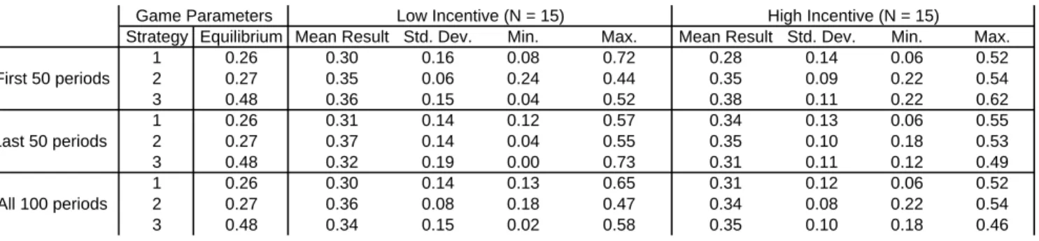
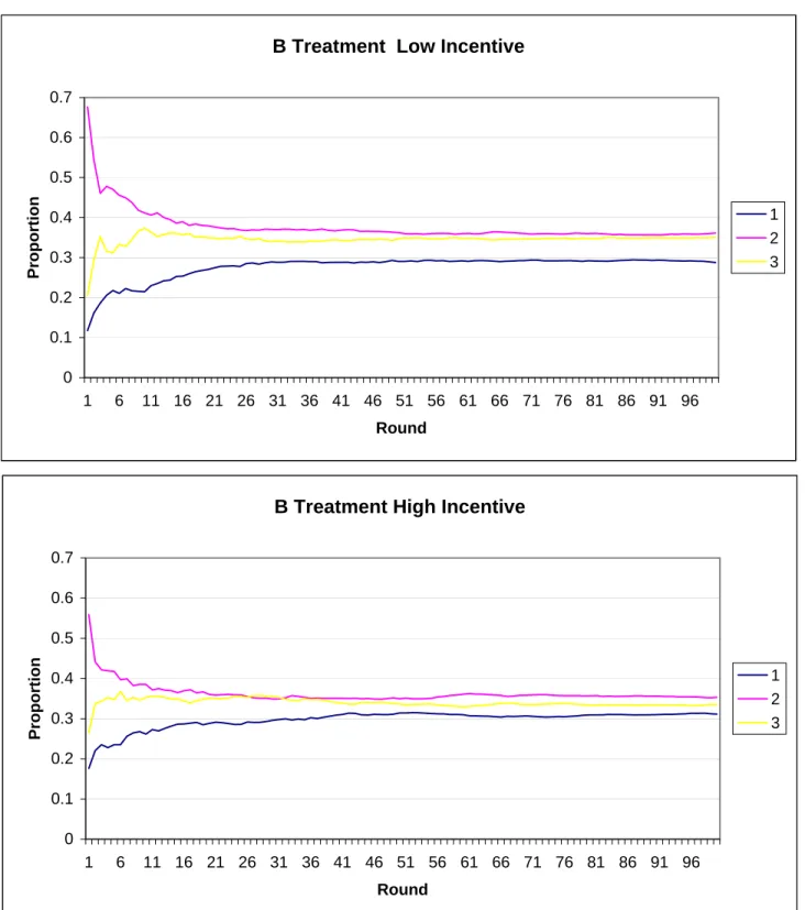
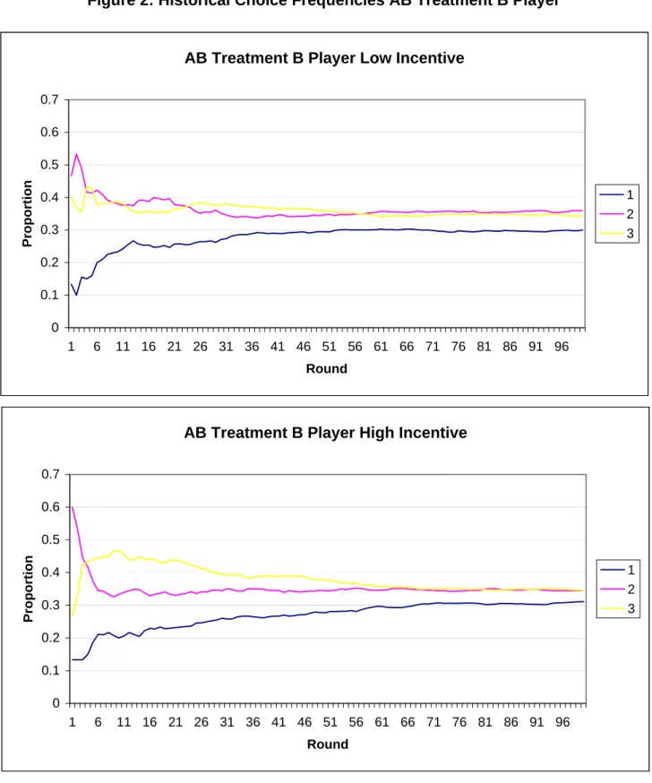
(20) treatments was the numbers presented to the subjects in the earnings table on the computer screen. Identical instruction sheets were used for all treatments. In fact, in principle it would have been possible to run multiple treatments in a session, but we did not do so. Subjects were told that they would make one-hundred decisions, and that the participant with whom they were randomly paired would stay the same throughout the entire session. They were informed that they would be paid for a randomly-chosen ten periods of play to be determined by the computer (to control for wealth effects). The subjects had to correctly answer questions on a quiz indicating that they understood how to read the earnings table, and that they understood that they did not know the content of their opponent’s earnings table. Subjects were then randomly assigned to the role of player 1 or player 2 (for example, to have the row payoffs or the column payoffs in game AB), though as noted above it was always presented to them that they were the row player. The sessions never lasted more than an hour and a half. A total of 128 subjects, who were English-speaking university students in Montreal, participated in the four experimental treatments. The experiment was programmed and conducted with the software z-Tree (Fischbacher 1999). The experiments were run in May and June, 2004 at the Bell Experimental Laboratory for Commerce and Economics at the Centre for Research and Analysis on Organizations (CIRANO). Subjects earned CAD $10.00 for showing up on time and participating fully (our show-up fee must take into account the fact that the laboratory is not on campus), and an average of $23.90 for the results of their decisions and the decisions of their opponent. Alternative opportunities for pay in Montreal for our subjects is considered to be approximately $8.00 per hour.. 6 6.1 6.1.1. Experimental Results Data and Data Analysis Aggregate Statistics. Tables 1 and 2 present the basic summary statistics from BB and AB treatments, where Table 2a presents results for B players and Table 2b for A players. The three main sections of the table, which are divided into rows, show the proportion of times subjects played each strategy in the first 50, last 50, and all 100 periods of the game, averaged over 34 subjects; the statistics presented are averages of individual player averages. The table is further divided into three sections from left to right: mixed-strategy equilibrium predictions, results from the low-incentive treatment, and results from the high-incentive treatment. The table shows that the mean frequencies are close to equilibrium in all 17.

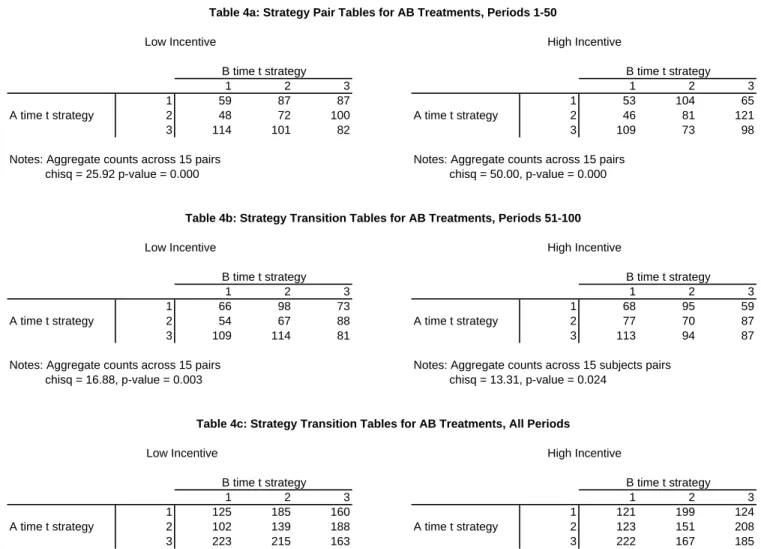
(21) cases. For example, across all 100 periods of the game strategies 1, 2, and 3 were chosen with a mean frequency of 0.29, 0.36 and 0.35 in the low-incentive BB treatment, and ˆ B. ˆ This compares with the mixed0.31, 0.35, and 0.34 in the high-incentive treatment B strategy equilibrium 0.28, 0.32, and 0.35 for both treatments, and this result is similar across the sessions and treatments. In the case of AB, B players overweight strategies 1 and 2 with respect to equilibrium, and underweight strategy 3. By contrast the mean frequencies of play of the A players are very close to equilibrium in both high and low payoff treatments.7 One of the principal questions is whether the time average of play is convergent. Figures 1-3 show the average of strategy choices for games BB and AB for both the low and high incentive treatments over time. The figures were generated by counting the number of times each player had chosen each of her three strategies throughout the entire game for each round in the game, then averaging the choices across players. The figures primarily show stability of choices during the sessions: play converges after approximately 25 periods of play in both treatments. The averages for all three strategies are similar between high and low incentive treatments in both the AB and BB games after 100 periods, despite being different at the start of the game. Players’ marginal frequencies are equally important but are not directly observable. We attempt to establish an approximate pattern for them by dividing the data on choices into ten period blocks. In Figures 4-6, the vertical axis gives the frequencies of choices of the three strategies and the horizontal axis corresponds to ten blocks of ten periods each. That is, the first block gives the decisions made in the first ten periods averaged over all subjects. These figures seem to indicate that marginal choice frequencies are reasonably stable over time. Average data could hide considerable heterogeneity at the level of individual pairs. However, if one looks at Tables 1 and 2, standard deviations are stable over time and are similar in AB and BB treatments. Tables 3 and 4 present 3 × 3 aggregate strategy pair tables for the BB and AB treatments. The row in each table represents the strategy played by a player at time t, and the column represents the strategy played by her opponent at time t. Each cell in the table is a count of number of times the corresponding strategy pair occurred in the data, summed across periods and all subject pairs. For example, the top section of Table 2 indicates that strategy pair LL occurred in the first 50 periods of the low-incentive treatment 55 times, and in the high-incentive treatment 84 times. Below the table is the chi-squared test statistic for independence between rows and columns (where a low p-value implies rejection of the null hypothesis of independence). The left table always represents the low-incentive treatment and the right table represents the high-incentive 7 The differences and similarities between the empirical and empirical frequencies are not in fact very well explained by QRE analysis (see the estimates of QRE for AB and BB in Section 4.3) even though it has had much success in other games (see McKelvey and Palfrey (1995)). The fit might be improved by taking into account risk aversion (Goeree et al., (2003)) but as our main focus here is on the dynamics of play, this is not something we have explored.. 18.

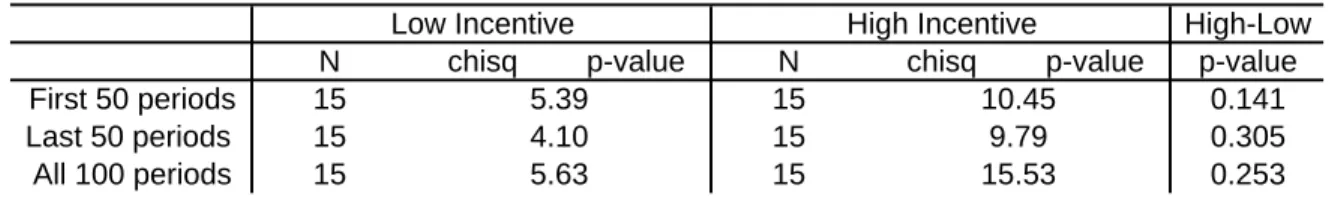
(22) treatment. The sub-tables a, b, and c present results from the first 50, last 50, and all 100 periods of the game. In the BB games (Table 3), we detect a difference within the high-incentive treatment and across both the low- and high-incentive treatments. We reject independence in the low-incentive treatment both in the first and last half of the session. However, we do not reject independence in the first half of the high-incentive treatment, and then we do reject independence in the second half. Thus the frequency tables suggest that, when summing over all subject pairs in the sessions, play between subjects is never independent with low incentives and loses its independence over time with high incentives. Table 4 presents 3 × 3 aggregate strategy pair tables for the AB treatments. In all cases, i.e., for both player types and in both the beginning and end of the game we reject independence of play between the row and the column players. Recall that in the BB treatments, play was independent early in the high-incentive treatment. 6.1.2. Analysis by subject pair. Tables 5 and 6 further explore correlated play, this time on a pair-by-pair basis. We computed the same chi-squared statistic for independence between the actions of row players and column players and interpreted it as a measure of the distance the play of a subject pair was from independence for each player pair in each treatment. We conducted Wilcoxon-Mann-Whitney tests for differences in this statistic between the two treatments. For example, in the first 50 periods of the low-incentive treatment the average chi-squared statistic was 7.17; in the high-incentive treatment it was 4.38; and the p-value of the Wilcoxon-Mann-Whitney test for the difference between treatments was 0.117. Tables 5 and 6 show that the mean chi-squared statistic increased from the first to the last half of the session for the B treatment, but declined slightly for the A treatment. In the B treatment (Table 5), there was nearly a statistical difference between high and low payoff treatments in the first 50 periods of the game, with a distance closer to independence in the high incentive treatment (p-value 0.117). The difference between treatments evaporated in the second half of play. This analysis, which takes into account subject pair heterogeneity, is consistent with the aggregate results previously discussed: play is less independent at the start of the low-incentive treatment and becomes nonindependent with time in both treatments. Table 6 shows that in the AB games the magnitude of the mean chi-squared statistic increased from the low- to the high-incentive treatment in both the first and last half of the session, but not significantly so. The bottom line resulting from this analysis is that play is correlated across opponents in all of our treatments. We explore the most likely explanation for this in the next subsection.. 19.

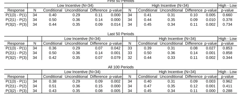
(23) 6.1.3. Best response cycles. If play is not independent across time or across opponents, then the most likely alternative explanation is that subjects are playing best-response cycles. In the BB treatments, best response cycles call for the following responses to opponent play in the previous period: 1 if the opponent plays 3; 2 if the opponent plays 1; 3 if the opponent plays 2. We estimated the conditional probability of each of the three responses in the cycle, and then subtracted the unconditional probability of playing the best response for each subject. That is, we computed Pr(1|3) − Pr(1), Pr(2|1) − Pr(2), Pr(3|2) − Pr(3). If subjects’ choices are independent of their opponent’s last choice, then these differences will be zero. If they are cycling, the differences will be positive. The results for the BB treatments are presented in Table 7. The table shows the conditional probability, the unconditional probability, the difference between the two measures, and the p-value of the t-test that this difference is zero. At the far right of the table we show the p-value of the Wilcoxon-Mann-Whitney test for a difference between experimental treatments. The table shows that all best responses are statistically significant no matter how we cut the data and no matter the treatment. The table also shows no statistical difference between any period of play or any treatment. Table 8 presents results from tests for best-response cycling in the AB treatments, with Table 8a presenting results for B players and Table 8b for A players. The only difference between these tables and Table 7 is the Player A best response pattern: 1 if the opponent plays strategy 1; 2 if the opponent plays strategy 2; and 3 if the opponent plays strategy 3. Table 8a shows that B players have a tendency to play their cycle, as they did in the BB treatments. In every case the difference between the conditional and conditional choice frequencies is statistically higher than zero (t-tests). By contrast with B-player behavior in the BB treatments, there is a statistical difference for two of the three best responses (with the third best response having a p-value of 0.133) between the high and low incentive treatments during the first 50 periods of play. This result goes away in the second 50 periods of play. Table 8b shows that in most cases the A players cycle as well. As with the B-players, there is evidence for a difference between the two treatments with two out of three of the best responses in the cycle. Unlike the B-players this difference persists throughout all 50 periods of the game. In Table 9 we compare cycling across treatments. We test whether the behaviour of B-players in AB treatments is different from the behaviour of B-players in BB treatments. In most cases, the differences are not significant. However, there is evidence that cycling is more pronounced in the high incentive AB treatment than in the high incentive BB treatment initially, but the difference is not significant in the second half of the data, nor overall. 20.

(24) We conclude from the analysis in this section that (1) players have a strong tendency to play their best-response cycles, (2) B-players cycle more in the high incentive treatment early in the game, but that the difference induced by high incentives goes away with experience in the game and (3) that A-players cycle more in the high incentive treatment throughout the game. These results contradict the theoretical predictions. 6.1.4. Regression analysis. For one final look at the data we ran a multinomial regression on each half-session of data separately. In the regressions the dependant variable is the decision at time t, and the independent variables are dummies for each of the three opponent’s strategies at time t − 1. We clustered on the subject id number for the purpose of computing the standard errors. The regression reports the probability of playing a strategy conditional on the various independent variables. Rather than report the regression output directly, for simplicity we present a grid in which we place an “X” whenever a strategy is significantly more probable than another strategy. For example, the right-most column in the top of Table 10 shows that in periods 1-50 in the low-incentive treatment, strategy 3 was more likely to be played than either strategy 1 or 2 whenever the opponent played strategy 2 at time t − 1. The two X’s that represent this result are both bold-faced to show that they are consistent with a bestresponse cycle. The table provides evidence that whenever an opponent’s one-period lagged strategy affects decision-making, it is overwhelmingly likely for the response to be on a best-response cycle. And several best-response cycles are represented by the behavior that generated this table. Table 11 shows results from the multinomial regressions for the AB games. Table 11a shows statistically significant responses to opponent actions at time t − 1 for B players, and Table 11b presents the same results for A players. As in the BB treatments, the tables show many responses to opponent actions and most of them are on a best-response cycle. There appear to be more of these responses by B players than A players, and this is consistent with results presented in the previous subsection.. 6.2. Comparison of Results with the Theoretical Hypotheses. The first thing to observe is that Figures 1-3 indicate that the time average of play in ˆ and B ˆB ˆ converges. Divergence would imply persistent all four treatments AB, BB, AˆB cycles in the data, giving radically different values in different time periods and different sessions. Notice that the time averages after 50 periods do not change substantially over ˆ B. ˆ This leads us to reject divertime. There is also little difference between BB and B gence of the time averages and, hence, also Hypothesis 1(b). It is true that the figures use aggregated data. However, the summary statistics including standard deviation in 21.

(25) ˆB ˆ than Table 1 do not indicate any greater dispersion amongst individual subjects in B in BB or than in the AB treatments. Convergence of the time average is consistent with Hypotheses 2 and 3. Of course, as we noted in Section 3, convergence in time average does not imply convergence in behaviour. We cannot directly observe the marginal frequencies of different strategies employed by each subject. However, Figures 4-6 that report choice frequencies in ten period blocks give no indication of non-stationarity in choices. Divergence in behaviour would imply considerable and increasing variation between blocks in choice frequencies. This we do not see. Again, subject heterogeneity may be hidden by aggregation. However, again the standard deviations reported in Table 1 indicate that play is not more dispersed in the BB treatments than in AB. The third major observation is that both types of correlation of play, across time and across opponents, are present. Intertemporal correlation is indicated by Tables 79 to be found in all treatments. If subjects randomised independently of each other, then we would expect little difference between the unconditional probability of playing an action and the probability conditional on the opponent’s previous action. Instead, Tables 7 and 8 indicate that subjects often played a best response to the previous action of their opponent. Similarly, in Tables 10-11 we have a number of significant coefficients, indicating both a lack of independence and, again, a tendency to best respond. This would lead to a rejection of Hypotheses 1(a) and 3(a) which suggest that there should be convergence in behaviour. Evidence on contemporaneous correlation between opponents is found in Tables 3-6. The chi-squared statistic leads us to reject independence of play between row and column players very strongly in all cases except the low incentive stable treatment (Table 6). This evidence again is not consistent with Hypotheses 1(a) and 3(a). Hypothesis 2(b) based on learning theory includes the claim that there should be ˆB ˆ than in BB than in the AB treatments. Hypothesis greater evidence of cycling in B 3(b) claims there should not. If we compare Tables 3c and 4c, then there appears not to ˆB ˆ or between BB and AB in that, be too great a difference, either between BB and B in all cases, play of row and column players seems to be heavily correlated. Similarly, an examination of Tables 5 and 6, would lead us to reject iid play over the 100 periods in all cases, except perhaps in the low incentive stable treatment AB. Further, Table 9 that directly compares AB and BB treatments finds only one significant difference in cyclical behaviour over the complete experiment (and this is in the wrong direction). Thus, if we look at statistics for the complete 100 periods, Hypothesis 3(b), that there is no great difference between the (supposed) stable and unstable games, fares best. However, if we compare the differences over time, we see a different picture. First, looking at Table 3, compare the chi-squared statistics for the first 50 periods with those for the second half of the experiments. While there is little change in BB, cycling seems ˆB ˆ from the first 50 periods to the second. Table 4 to have increased considerably in B 22.

(26) ˆ While the chi-squared provides evidence for the opposite effect in games AB and AˆB. scores indicate that we reject independence both in the first and second half of the data, the level of correlation has decreased over time. We find a similar pattern in Tables 5 and 6. The average level of correlation increases from the first to the second half in both BB treatments but decreases in both AB treatments. These results are consistent with ˆ subjects get closer to equilibrium a learning story: in the stable games AB and AˆB, play over time, so that correlation decreases over time (however, the level of correlation ˆ in Table 6 remains high). In B ˆ B, ˆ however, learning takes players displayed in AˆB further from equilibrium, and the cycling becomes more pronounced. This is supportive of Hypothesis 2(b). In summary, we can reject both strict equilibrium play, that is, independent randomisation, and complete divergence. This is enough to cast doubt on both classical learning models (Hypotheses 1(a) and 1(b)) and the simple assumption that subjects always play equilibrium (Hypothesis 3(a)). However, while we find significant evidence for best response cycles in all treatments, there is some evidence that these cycles weaken ˆ B. ˆ This is consistent with over time in the AB treatments, but strengthen over time in B converging learning in the first case, and diverging learning in the second. Thus, there is some support for the learning hypotheses 2(a) and 2(b). However, the differences between the stable and unstable treatments are not very strong and so it is difficult to rule out Hypothesis 3(b), that is, there is weak convergence to equilibrium in all the games.. 7. Conclusions. We tested the theoretical possibility, first discovered by Shapley (1964), that in some games learning fails to converge to any equilibrium, either in terms of marginal frequencies or of average play. Subjects played repeatedly in fixed pairings one of two classes of 3 × 3 game, each having a unique Nash equilibrium in mixed strategies. The equilibrium in one class of games is predicted to be stable under learning, in the other class unstable. Thus, if we take learning theory seriously, play should be more dispersed in the second class. Furthermore, in the second class, there should be greater correlation of play both across time and across players. Our experimental design provided a tough test of the theory by studying play in fixed pairings. This potentially allowed players to attempt to collude, which would conflict with the myopic maximisation assumed by fictitious play. However, the lack of information about opponents’ payoffs seems to have successfully prevented collusive behaviour. Otherwise, by providing the subjects with the entire history of play as well as history of marginal choice frequencies, the design kept the subjects well informed. One conjecture would be that withholding information on past choices might encourage more divergent behaviour in unstable games. 23.

(27) As it was, the performance of the theory was mixed. Play in both classes of games was on average not too far from equilibrium. However, we found play from round-toround not to be independent in either treatment. On some measures it looks as though that play is more strongly correlated in the unstable class of game than in the stable and this would be consistent with the theory. But it is not possible to make a clear distinction between the stable and unstable cases, as strong correlation is present in all treatments. As is often the case, theoretical predictions that are clearly different on the page are not so distinct once one tries to reproduce them in the laboratory. This highlights a more general point. Theorists typically obtain results in complex models by taking limits. In this case, stochastic fictitious play seems to predict significant differences in behaviour between the stable and unstable games. However, this is only really true for parameter values being close to their limit values, in particular the level of noise must be sufficiently small and memory must be sufficiently long. In practice, the observed differences are much smaller than the apparent theoretical predictions. However, this is still consistent with the predictions of the model but with a high level of noise and with a short memory. This is consistent with the findings of Camerer and Ho (1999) whose estimates of similar learning models find parameter values far from their limiting values. This is also consistent with the findings of the literature on logit equilibrium (see Anderson et al. (2002) for a survey) that explains significant and persistent deviation from Nash equilibrium play on the basis that noise is nonvanishing. We present evidence here that similar considerations hold for dynamics as well as equilibrium behaviour. If one wants to predict the dynamics of play, one should also take into account that noise is substantial and correlation is persistent.. Appendix Most of the theoretical results follow from application of the theory of stochastic approximation. Note that that, given the updating rules (14) or (15), the expected change in beliefs can be written E[bimn+1 |bn ] − bimn = γn (pimn − bimn ), for m = 1, ..., 3. (16). where γn is the step size (equal to 1/(n + t) under fictitious play beliefs, equal to 1 − δ under recency). In the terminology of stochastic approximation, the associated system of ordinary differential equations (ODE) can be written in vector form as b˙ i = φ(bj ) − bi , b˙ j = φ(bi ) − bj .. (17). It is possible to predict the behaviour of the stochastic learning process by the analysis of the behaviour of these ODE’s. Proof of Proposition 1: In this game, the perturbed equilibrium is unique and globally stable under the associated ODE (17) by Theorem 3.2 of Hofbauer and Hopkins (2005). 24.