Behrens: Department of Economics, Université du Québec à Montréal (UQAM) and CIRPÉE, Canada; CEPR, UK [email protected]
Murata: Advanced Research Institute for the Sciences and Humanities (ARISH), Nihon University, 12-5, Goban-cho, Chiyoda-ku, Tokyo 102-8251, Japan; and Nihon University Population Research Institute (NUPRI), Japan
Cahier de recherche/Working Paper 09-40
Trade, Competition, and Efficiency
Kristian Behrens Yasusada Murata
Abstract:
We present a general equilibrium model of monopolistic competition featuring pro-competitive effects and a pro-competitive limit, and investigate the impact of trade on welfare and efficiency. Contrary to the constant elasticity case, in which all gains from trade are due to product diversity, our model allows for a welfare decomposition between gains from product diversity and gains from pro-competition effects. We then show that the market outcome is not efficient because too many firms operate at an inefficiently small scale by charging prices above marginal costs. Using pro-competitive effects and the competitive limit, we finally illustrate that trade raises efficiency by narrowing the gap between the equilibrium utility and the optimal utility.
Keywords: Pro-competitive effects, competitive limit, excess entry, trade and efficiency, monopolistic competition
1
Introduction
Few trade theorists would disagree with the statement that product diversity, scale economies, and pro-competitive effects are central to any discussion about gains from trade and efficiency with differentiated goods under imperfect competition.1 Yet, it is fair to say that these ques-tions have not been fully and jointly explored within a simple and solvable general equilibrium model of monopolistic competition.2 This is largely due to the fact that the workhorse ap-proach to international trade under monopolistic competition, namely the constant elasticity of substitution (henceforth, CES) framework, displays two peculiar features. First, it does not allow for pro-competitive effects so that “there is no effect of trade on the scale of production, and the gains from trade come solely through increased product diversity” (Krugman, 1980, p.953). Second, the equilibrium in the CES model is usually constrained (second-best) optimal, i.e., the market provides the socially desirable number of varieties at an efficient scale (Dixit and Stiglitz, 1977). Consequently, trade is not efficiency enhancing in the CES model because it does not correct the only existing market failure, pricing above marginal cost.
In order to more fully explore gains from trade and efficiency under monopolistic competi-tion, we must depart from the standard CES model. Doing so, however, has long been difficult since variable elasticity of substitution (henceforth, VES) models have “not proved tractable, and from Dixit and Norman (1980) and Krugman (1980) onwards, most writers have used the CES specification” (Neary, 2004, p.177). Building on the new general equilibrium model of monopolistic competition by Behrens and Murata (2007), we present a simple VES model of in-ternational trade featuring pro-competitive effects (i.e., profit-maximizing prices are decreasing in the mass of competing firms) and a competitive limit (i.e., profit-maximizing prices converge to marginal costs when the mass of competing firms becomes arbitrarily large). Within this framework, we investigate the impact of trade on welfare and efficiency.
Our results can be summarized as follows. First, unlike in the standard CES model, the market outcome is not efficient under autarky because too many firms operate at an inefficiently small scale by charging prices above marginal costs.3 Second, due to pro-competitive effects, markups in autarky are no longer the same across countries of different sizes. Nevertheless,
1Dixit (2004, p.128) summarizes the gains from trade under monopolistic competition as follows: (i)
avail-ability of greater variety; (ii) better exploitation of economies of scale; and (iii) greater degree of competition, driving prices closer to marginal costs. More recently, the World Trade Organization (2008, pp.48-50) provides a similar classification: (i) gains from increased variety; (ii) gains from increased competition; and (iii) gains from increased economies of scale.
2For instance, the World Trade Organization (2008, p.48) states that “(a)s far as the gains from
intra-industry trade are concerned, most studies have focused on either one of the variety, scale or pro-competitive (price) effects of trade opening”.
3Note that in a more general CES model, where market power and taste for variety are disentangled, the
equilibrium mass of firms can be larger or smaller than the optimal one (Benassy, 1996). However, that discrepancy is not due to pro-competitive effects because the model displays constant markups.
we show that free trade leads not only to the equalization of price-wage ratios but also to both product and factor price equalization, even when products are differentiated. Third, we concisely illustrate that trade leads to an increase in the mass of varieties consumed, and to a decrease in the mass of varieties produced in each country. In addition, we show that such exit of firms due to pro-competitive effects is accompanied by an increase in output per firm, which leads to a better exploitation of firm-level scale economies. Fourth, contrary to the CES case, in which all gains from trade are due to greater product diversity, our model allows for a welfare decomposition between gains from product diversity and gains from pro-competitive effects. Finally, using pro-competitive effects and the competitive limit, we illustrate that trade raises efficiency by narrowing the gap between the equilibrium utility and the optimal utility.
The remainder of the paper is organized as follows. Section 2 develops the model, and Section 3 focuses on the autarky case. Section 4 analyzes the trade equilibrium, decomposes the gains from trade, and shows that trade integration drives prices closer to marginal costs, thus enhancing efficiency. Section 5 concludes.
2
Model
Consider a world with two countries, labeled r and s. Variables associated with each country will be subscripted accordingly. There is a mass Lr of workers/consumers in country r, and
each worker supplies inelastically one unit of labor. Thus, Lr also stands for the total amount
of labor available in country r. We assume that labor is internationally immobile and that it is the only factor of production.
2.1
Preferences
There is a single monopolistically competitive industry producing a horizontally differentiated consumption good with a continuum of varieties. Let Ωr (resp., Ωs) be the set of varieties
produced in country r (resp., s), of measure nr (resp., ns). Hence, N ≡ nr+ ns stands for the
endogenously determined mass of available varieties in the global economy. A representative consumer in country r solves the following consumption problem, with ‘constant absolute risk aversion’ (CARA) sub-utility functions (Behrens and Murata, 2007):
max qrr(i), qsr(j) Ur ≡ Z Ωr £ 1− e−αqrr(i)¤di + Z Ωs £ 1− e−αqsr(j)¤dj s.t. Z Ωr prr(i)qrr(i)di + Z Ωs psr(j)qsr(j)dj = Er, (1)
where α > 0 is a utility parameter; Er stands for the expenditure; pr(i) denotes the price of
variety i, produced in country r; and qsr(j) stands for the per-capita consumption of variety j,
We show in Appendix A that the demand functions for country-r consumers are given as follows: qrr(i) = Er− 1 α Z Ωr ln · pr(i) pr(j) ¸ pr(j)dj− 1 α Z Ωs ln · pr(i) ps(j) ¸ ps(j)dj Z Ωr pr(j)dj + Z Ωs ps(j)dj , (2) qsr(j) = Er− 1 α Z Ωr ln · ps(j) pr(i) ¸ pr(i)di− 1 α Z Ωs ln · ps(j) ps(i) ¸ ps(i)di Z Ωr pr(i)di + Z Ωs ps(i)di . (3)
Mirror expressions hold for country-s consumers. Because of the continuum assumption firms are negligible, so that the own-price derivatives of the demand functions are given as follows:
∂qrr(i) ∂pr(i) =− 1 αpr(i) ∂qsr(j) ∂ps(j) =− 1 αps(j) , (4)
which then yields the variable demand elasticities εrr(i) = [αqrr(i)]−1 and εsr(j) = [αqsr(j)]−1.
Mirror expressions hold again for country s.
2.2
Technology
All firms have access to the same increasing returns to scale technology. To produce Q(i) units of any variety requires l(i) = cQ(i) + F units of labor, where F is the fixed and c is the marginal labor requirement. We assume that firms can costlessly differentiate their products and that there are no scope economies. Thus, there is a one-to-one correspondence between firms and varieties, so that the mass of varieties N also stands for the mass of firms operating in the global economy. There is free entry and exit in each country, which implies that nr and ns
are endogenously determined by the zero profit conditions. Consequently, the expenditure Er
equals the wage wr in country r.
International markets are assumed to be integrated, so that firm i ∈ Ωr sets a unique
free-on-board price pr(i) for consumers in both countries. Its profit is then as follows:
Πr(i) = [pr(i)− cwr] Qr(i)− F wr, (5)
where Qr(i)≡ Lrqrr(i) + Lsqrs(i) stands for its total output.
2.3
Equilibrium
Country-r (resp., country-s) firms maximize their profit (5) with respect to pr(i) (resp., ps(j)),
taking the vectors (nr, ns) and (wr, ws) of firm distribution and factor prices as given.4 This
4It is well known that price and quantity competition yield the same outcome in monopolistic competition
yields the following first-order conditions: ∂Πr(i) ∂pr(i) = Qr(i) + [pr(i)− cwr] · Lr ∂qrr(i) ∂pr(i) + Ls ∂qrs(i) ∂pr(i) ¸ = 0, (6) ∂Πs(j) ∂ps(j) = Qs(j) + [ps(j)− cws] · Ls ∂qss(j) ∂ps(j) + Lr ∂qsr(j) ∂ps(j) ¸ = 0. (7)
Conditions (6) and (7) highlight a fundamental property of monopolistic competition models: although each firm is negligible to the market, it must take into account the aggregate pricing decisions of the other firms since their prices enter its first-order condition.
We define a price equilibrium as a distribution of prices satisfying (6) and (7) for all i∈ Ωr
and j ∈ Ωs. We will discuss its existence, uniqueness, and some other properties in the following
sections.5
An equilibrium is a price equilibrium and vectors (nr, ns) and (wr, ws) of firm distribution
and factor prices such that national factor markets clear, trade is balanced, and firms earn zero profits. More formally, an equilibrium is a solution to the following three conditions:
Z Ωr £ cQr(i) + F ¤ di = Lr, (8) Z Ωs £ cQs(j) + F ¤ dj = Ls, (9) Ls Z Ωr pr(i)qrs(i)di = Lr Z Ωs ps(j)qsr(j)dj, (10)
where all quantities are evaluated at a price equilibrium. It is readily verified that firms earn zero profits when conditions (8)–(10) hold. One may set either wr or ws as the numeraire.
However, we need not choose a numeraire, since the model is fully determined in real terms.6
3
Autarky
Assuming that the two countries cannot trade initially with each other, we first characterize the equilibrium and the optimum in the closed economy, and show that there is excess entry in equilibrium. Without loss of generality, we consider country r in what follows.
5As shown by Roberts and Sonnenschein (1977), the existence of (price) equilibria is usually problematic in
monopolistic competition models, since firms’ reaction functions may be badly behaved. Because our model relies on a continuum of firms, which are individually negligible, we do not face this problem. In a similar spirit, Neary (2003) uses a general equilibrium model of oligopolistic competition with a continuum of sectors, in which firms are ‘large’ in their own markets but ‘negligible’ in the whole economy. This also allows to restore equilibrium since firms cannot directly influence aggregates of the whole economy.
6The choice of the numeraire is immaterial in our monopolistic competition framework. This is an important
departure from general equilibrium oligopoly models, where the choice of the numeraire is usually not neutral (Gabszewicz and Vial, 1972).
3.1
Equilibrium
Inserting (2)–(4) into (6), and letting qrs(i) = ∂qrs(i)/∂pr(i) = 0 and qsr(j) = ∂qsr(j)/∂ps(j) = 0,
one can show that the unique price equilibrium is symmetric and given as follows (see Behrens and Murata, 2007, for the proof):
par = µ 1 + α cna r ¶ cwar, (11)
where an a-superscript henceforth denotes autarky values. At the symmetric price equilibrium, the profit of each firm is given by Πar = Lrqarr(par − cwar)− F war. Using the consumer’s budget
constraint war = narparqrra, the above expression can be rewritten as
Πar = parqarr[Lr(1− cnarq a
rr)− F n a r].
Zero profits then imply that the quantities must be such that
qrra = 1 c µ 1 na r − F Lr ¶ , (12)
which are positive because narF < Lr must hold from the resource constraint when nar firms
operate. Utility is then given by
U (nar) = nar · 1− e−αc “ 1 nar− F Lr ”¸ . (13)
Note that (12) and (13) hold whenever prices are symmetric and firms earn zero profit. Inserting qa
rr = war/(narpar) into the labor market clearing condition (8), we get:
nar = Lr F µ 1− cw a r pa r ¶ . (14)
The equilibrium mass of firms can then be found by using (11) and (14), which yields:7
nar = p
4αcF Lr+ (αF )2− αF
2cF > 0. (15)
Finally, inserting (15) into (13), the equilibrium utility in autarky is given by
U (Lr) = p 4αcF Lr+ (αF )2− αF 2cF · 1− e− 2αF √ 4αcF Lr +(αF )2+αF ¸ > 0, (16)
which is a strictly increasing and strictly concave function of the population size Lr for all
admissible parameter values, i.e., α > 0, c > 0, F > 0, and Lr > 0.
3.2
Optimum
We now determine the socially optimal mass of varieties. The planner maximizes the utility, as given by (1), subject to the technology and resource constraints (8). The first-order conditions of this problem with respect to qrr(i) show that the quantities must be symmetric. This,
together with (8), implies that:
qrr = Qr Lr = 1 c µ 1 nr − F Lr ¶ . (17)
Hence, the planner maximizes
U (nor) = nor · 1− e−αc “ 1 nor− F Lr ”¸ , (18) with respect to no
r, where an o-superscript henceforth denotes the optimal values.8 Standard
calculations show that
∂U ∂no r = 1− µ 1 + α cno r ¶ e−αc “ 1 nor− F Lr ” (19)
and that U is a strictly concave function of no
r. Equating (19) to zero, utility maximization
requires the first-order condition
cno r α + cno r = e−αc “ 1 nor− F Lr ” =⇒ − µ 1 + α cno r ¶ e− “ 1+cnoα r ” =−e−1−cLrαF . (20)
By definition of the Lambert W function, the latter can be rewritten as9
− µ 1 + α cno r ¶ = W ³ −e−1−αF cLr ´ .
Solving this equation for no
r yields a unique optimal mass of firms
nor =− α c h 1 + W−1 ³ −e−1−cLrαF ´i > 0, (21)
where W−1 is the real branch of the Lambert W function satisfying W (−e−1−αF /(cLr)) ≤ −1
(Corless et al., 1996, pp.330-331).10 Note that W
−1 is increasing in Lr and that −∞ < W−1 <
−1 for 0 < Lr <∞. Furthermore, using (20) we can show the following excess entry result.
Proposition 1 There are too many firms operating at an inefficiently small scale in equilibrium,
i.e., na r > nor.
Proof. See Appendix B.
8As shown in Behrens and Murata (2006, Appendix B), alternative policies: (i) marginal cost pricing and
lump-sum transfers; and (ii) profit-maximizing prices and non-negative profits, boil down to the same problem.
9Formally, the Lambert W function is defined as the inverse of the function x7→ xex (Corless et al., 1996).
10As−e−1 <−e−1−αF /(cLr)< 0, there is another possible real value of W (−e−1−αF /(cLr)) satisfying−1 <
W (−e−1−αF /(cLr)) < 0. However, it leads to no
Note that excess entry arises because of pro-competitive effects (∂pa
r/∂nar < 0 by (11)). The
negative externality each firm imposes on the other firms gives rise to the ‘business-stealing effect’ (Mankiw and Whinston, 1986, p.49), i.e., the equilibrium output per firm declines as the number of firms grows (∂Qa
r/∂nar = ∂(Lrqarr)/∂nar < 0 by (12)).
Interestingly, this result contrasts starkly with the constant elasticity case, where the equi-librium mass of varieties is (second-best) optimal.11 Stated differently, the basic CES model does not account for the tendency that too many firms produce at inefficiently small scale in autarky (the so-called ‘Eastman-Stykolt hypothesis’; Eastman and Stykolt, 1967), an argument often used to criticize import-substituting industrialization policies (Krugman and Obstfeld, 2003, pp.261-263) or tariff barriers (Horstmann and Markusen, 1986) on efficiency grounds.
Finally, combining (18) and (20) yields Uo(no
r) = αnor/(α + cnor). Inserting (21) into this
expression, the optimal utility is given by
Uo(Lr) = − α cW−1 ³ −e−1−αF cLr ´ > 0, (22)
which is a strictly increasing function of the population size Lr for all admissible parameter
values, i.e., α > 0, c > 0, F > 0, and Lr > 0.
4
Free trade
We now analyze the impacts of trade on welfare and efficiency in a world with pro-competitive effects and a competitive limit. Section 4.1 analyzes the equilibrium. Section 4.2 then shows the existence of gains from trade and decomposes them into gains from product diversity and gains from pro-competitive effects. Section 4.3 finally illustrates that trade narrows the gap between the equilibrium utility and the optimal utility by driving prices closer to marginal costs.
4.1
Equilibrium
We have shown that the profit-maximizing price under autarky is given by (11), where na r is
given by (15). Therefore, unlike in the standard CES model, markups in autarky are no longer the same across countries of different sizes. Nevertheless, we now show that free trade leads not only to the equalization of price-wage ratios, but also to product and factor price equalization. Assume that both countries can trade freely. The profits and the first-order conditions are still given by (5)–(7), respectively. Using these expressions, we establish the following proposition.
11This can be seen from Dixit and Stiglitz (1977, p.301), when letting s = 1 and θ = 0 in their equations
(20) and (21), since there is no homogeneous good in our setting. Note that the two-factor two-sector CES trade model by Lawrence and Spiller (1983, p.68) even displays insufficient entry. This runs against the general tendency of excess entry obtained under “a range of very plausible situations” (Vives, 1999, p.176).
Proposition 2 Free trade leads to product and factor price equalization for all admissible
pa-rameter values.
Proof. See Appendix C.
Note that there is a priori no reason for product price equalization to hold in our setting, even under free trade.12 This is because firms sell differentiated varieties, factor markets are segmented, and firms are imperfectly competitive.
From Proposition 2, we know that pr = ps = p and wr = ws = w, which allows us to rewrite
(2)–(4) as follows: qrr= qsr = qss= qrs = w N p (23) and ∂qrr ∂pr = ∂qsr ∂ps = ∂qss ∂ps = ∂qrs ∂pr =− 1 αp. (24)
Inserting (23) and (24) into the first-order condition (6), we obtain the price equilibrium:
p = ³ 1 + α cN ´ cw, (25)
which is an extension of the autarky case (11). Since prices and wages are equalized, all firms sell the same total quantity Q = (Lr + Ls)q. Labor market clearing then implies that
nr/ns = Lr/Ls, which yields nr = Lr F µ 1−cw p ¶ . (26)
Plugging (25) into (26) and the analogous expression for country s, we obtain two equations with two unknowns nr and ns. Solving for the equilibrium masses of firms, we get
nr = Lr Lr+ Ls p 4αcF (Lr+ Ls) + (αF )2− αF 2cF ns = Ls Lr+ Ls p 4αcF (Lr+ Ls) + (αF )2− αF 2cF .
Thus, the equilibrium mass of firms in the global economy is given by
N = nr+ ns =
p
4αcF (Lr+ Ls) + (αF )2 − αF
2cF , (27)
which is an extension of the autarky expression (15). It is readily verified that N > max{na r, nas},
thus implying that p/w < min{par/wra, pas/was} from (11) and (25). Finally, from expressions
(14) and (26), we obtain nr < nar and ns < nas. Hence, the relationship between trade and
product diversity can be summarized as follows:
Proposition 3 When compared with autarky, the mass of varieties produced in each country
decreases under free trade, whereas the mass of varieties consumed in each country increases.
12Most studies assume, rather than prove, that product price equalization holds under free trade (e.g.,
Proposition 3 illustrates exit of firms due to the pro-competitive effects of international trade. Once trade occurs, the price-cost margins in both countries decrease, thus driving some firms out of each national market (Krugman, 1979; Feenstra, 2004, Ch.5).13 Factor market clearing then makes sure that firm-level and total production expands, as labor is reallocated from the fixed requirements of closing firms to the marginal requirements of surviving firms. This is an important departure from the CES model, in which such an effect does not arise. Note also that Proposition 2 holds regardless of country size. In autarky, a smaller country tends to have a smaller mass of firms, which implies a higher price-wage ratio. Therefore, the price-wage ratio in a small country decreases more than that in a large country under free trade, i.e., we observe convergence in price-wage ratios across countries.
Note, finally, that although there is a growing literature on firm heterogeneity in interna-tional trade (e.g., Melitz, 2003), the price-cost margin for each firm is usually assumed to be constant in these models because of the CES specification.14 By contrast, our model captures the ‘old idea’ that international trade under imperfect competition leads to lower markups and hence to exit of firms even without firm heterogeneity (Dixit and Norman, 1980).
4.2
Welfare decomposition and gains from trade
We now discuss gains from trade by decomposing welfare as in Krugman (1981). Since varieties are symmetric under both free trade and autarky, the utility difference is given by:
Ur− Uar = N ³ 1− e−αwN p ´ − na r µ 1− e− αwar nar par ¶ .
Adding and subtracting nare−αw/(narp), and rearranging the resulting terms, we obtain the
fol-lowing welfare decomposition:
Ur− Uar = N ³ 1− e−αwN p ´ − na r ³ 1− e−naαwr p ´ | {z } Product diversity + nar ³ e− αwar nar par − e− αw nar p ´ | {z } Pro-competitive effects , (28)
which isolates the two channels, namely product diversity and pro-competitive effects, through which gains from trade materialize in our model.
We now examine the role and the sign of each component in expression (28) in more details, both from a theoretical and an empirical point of view.
13In Lawrence and Spiller (1983, Proposition 7), international trade leads to a redistribution of existing firms
between the two countries while the total mass of firms remains unchanged. This result is driven by changes in relative factor prices under free trade and, as pointed out by the authors, need not hold under variable markups.
14One notable exception is Melitz and Ottaviano (2008) who recently proposed a model that explains
trade-induced exit by combining pro-competitive effects and firm heterogeneity in a quasi-linear framework. Yet, the quasi-linear specification rules out income effects and gives their model a partial equilibrium flavor.
Product diversity: As shown in Proposition 3, trade expands product diversity, as in the CES case, despite the exit of some domestic producers. Ceteris paribus this raises utility via ‘love-of-variety’, which can be seen as follows. Given the wage-price ratio under free trade,
w/p, we have Ur = N ³ 1− e−αwN p ´ , ∂Ur ∂N = 1− e −αw N p µ 1 + αw N p ¶ > 0 ∀N.
To obtain the last inequality, let z≡ αw/(Np) and h(z) ≡ 1−e−z(1 + z). Clearly, h(0) = 0 and
h0(z) > 0 for all z > 0, which shows that for any given wage-price ratio w/p, utility increases with the range of varieties consumed.
Despite its central theoretical role in new trade theory, little is known until now about the empirical importance of gains from product diversity (Feenstra, 1995). Using extremely disaggregated data, Broda and Weinstein (2006) document that the number of product varieties in US imports rose by 212% between 1972 and 2001, and according to their estimates this maps into US welfare gains of about 2.6% of GDP. This finding suggests that product diversity is an important real-world channel through which gains from trade materialize.
Pro-competitive effects: The second term in (28) captures the beneficial effects of increased price competition in the product market, driving prices closer to marginal costs. This can be seen by comparing expressions (11) and (25). Note that wa
r/par = w/p would hold in the CES
case, i.e., there would be no gains from trade due to pro-competitive effects.
It is well known from various industrial organization studies that prices in many imperfectly competitive industries are increasing functions of producer concentration (see Schmalensee, 1989, pp.987-988, for a survey). In our symmetric equilibrium, the Herfindahl-index of con-centration, defined as the sum of squared market shares, reduces to H = N (1/N )2 = 1/N . Since the mass of firms is increasing in market size in our model, markups are lower in larger markets (see Campbell and Hopenhayn, 2005, for empirical evidence). Similarly, by increas-ing the number of competitors in each market, import competition decreases concentration, which maps into lower consumer prices. Several case studies confirm this ‘imports-as-market-discipline hypothesis’ (e.g., Levinsohn, 1993; Harrison, 1994; Tybout, 2003). More recently, Badinger (2007) finds solid evidence that the Single Market Programme of the EU has reduced markups by 26% in aggregate manufacturing of 10 member states.
Let us summarize our results as follows:
Proposition 4 Free trade raises welfare both by expanding consumers’ choice sets (‘product
diversity’) and by driving prices closer to marginal costs (‘pro-competitive effects’).
Proof. To prove our claim, it is sufficient to examine the sign of the two components in (28). As shown above, they are both positive, which ensures gains from trade.
4.3
Competition and efficiency
In Section 3.2 we have considered the case in which each national government maximizes its own welfare under its domestic resource constraint (‘decentralized’ first-best). As shown by Behrens and Murata (2006, Appendix D), doing so is equivalent to letting a global planner maximize world welfare under a global resource constraint (‘centralized’ first-best). Put differently, if no r
and nos is a decentralized optimum, then No = nor+ nos is a centralized optimum. Conversely, if No is a centralized optimum, then no
r = (Lr/L)No and nos = (Ls/L)No is a decentralized
optimum, where L≡ Lr+ Ls. The optimal utilities under both regimes are the same.
Since in our model free trade amounts to increasing the population size, the result on excess entry established in Section 3.2 continues to hold, even under free trade. Stated differently, there is a unique optimal mass of firms No< N satisfying the first-order condition (20) under
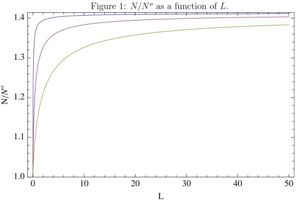
free trade. Hence, there are too many firms operating at an inefficiently small scale and the market outcome is not efficient. Figure 1 depicts a typical example of N/No as a function of
L.15 It shows that excess entry gets larger as population increases. Yet, for any given value of
L, the smaller the value of α the narrower the gap between the equilibrium and the optimum.
Furthermore, limL→0N/No = 1 and limL→∞N/No =
√
2 hold regardless of parameter values.
[Insert Figure 1 around here]
On the contrary, combining (25) and (27) we obtain pro-competitive effects as follows:
p cw = 1 + 2αF p 4αcF L + (αF )2− αF and ∂ ∂L ³ p cw ´ < 0. (29)
It is then readily verified that our model exhibits a competitive limit
lim L→0 p cw =∞ and Llim→∞ p cw = 1,
so that prices converge to marginal costs as population gets arbitrarily large. Despite the fact that excess entry tends to get worse as population increases, such losses are dominated by efficiency gains from the competitive limit, thus yielding the following efficiency result.16
Proposition 5 When the population gets arbitrarily large in the integrated economy, the
equi-librium utility converges to the optimal utility, i.e.,
lim
L→∞U (L) = limL→∞U
o(L) = α
c.
15The parameter values are as follows: α = 0.1, 1, 5 from above; c = 0.5; and F = 1. Other admissible
parameter values yield qualitatively similar figures, thus suggesting that the underlying property is robust.
16This result is reminiscent of Mankiw and Whinston (1986, Proposition 3) who establish conditions for the
Proof. Applying the l’Hospital’s rule to (16), it is readily verified that limL→∞U (L) = α/c.
Furthermore, by definition of the Lambert W function, limL→∞W−1(−e−1−αF/(cL)) =−1 holds.
Hence, taking the limit of expression (22) yields limL→∞Uo(L) = α/c.17
The limit result established in Proposition 5 may be extended to a finite economy by inves-tigating whether max ½ U (Lr) Uo(L r) , U (Ls) Uo(L s) ¾ < U (L) Uo(L) < 1, (30)
where the last inequality comes from the definition of the optimum. To this end, we check whether the ratio of equilibrium to optimal utility U/Uo monotonically increases in L. This is
not a trivial question since both the equilibrium and the optimal utility increase in L, as can be seen from (16) and (22).
[Insert Figure 2 around here]
Figure 2 depicts a typical example of U/Uo as a function of L.18 As U/Uo < 1 the market
outcome remains inefficient for finite population sizes. However, for any given value of L, the smaller the value of α, the narrower the gap between the equilibrium and the optimum. The reason is that a smaller value of α implies lower p/(cw) for all L by (29). Furthermore, since
U/Uo increases monotonically with L, trade between larger countries yields higher efficiency
than trade between smaller countries.
5
Conclusions
We have developed a VES model of international trade displaying pro-competitive effects and a competitive limit and investigated the impact of trade on welfare and efficiency. First, we have shown that, unlike in the standard CES model, there is excess entry due to pro-competitive effects. Second, even in the presence of pro-competitive effects and product differentiation, free trade leads to product and factor price equalization between countries of different sizes. Third, we have illustrated the well-known property that trade leads to an increase in the mass of varieties consumed, and to a decrease in the mass of varieties produced, in each country. In addition, we have shown that exit due to pro-competitive effects is accompanied by an increase in output per firm because of resource reallocation from the fixed to the marginal labor requirement, leading to a better exploitation of firm-level scale economies. Fourth, contrary to the CES case, our model allows for a welfare decomposition between gains from product diversity and gains from pro-competitive effects. Finally, we have illustrated that trade is
17See Behrens and Murata (2006, Appendix E) for an alternative proof without using the Lambert W function. 18The parameter values are as follows: α = 0.1, 1, 5 from above; c = 0.5; and F = 1. Other admissible
parameter values yield qualitatively similar figures, thus suggesting that the underlying property is robust. Furthermore, limL→0U/Uo= 1− e−1≈ 0.63 holds regardless of parameter values.
efficiency enhancing through increased competition. In particular, as the population size gets arbitrarily large in the integrated economy, the equilibrium utility converges to the optimal utility because of a competitive limit.
The framework presented in this paper is flexible enough to allow for many extensions, including heterogeneous firms and trade costs (Behrens et al., 2009) and heterogeneous con-sumers (Behrens and Murata, 2009). The next step is to extend our model to a multi-sector setting in order to fully explore the impact of trade on efficiency. In our model, trade tends to reduce within-sector efficiency losses, which disappear at the competitive limit. However, as is well known, markup heterogeneity across sectors is a source of between-sector distortions (Bilbiie et al., 2008; Epifani and Gancia, 2009), which may become more important with freer trade. Whereas Epifani and Gancia (2009) show that trade may reduce efficiency, the existence of a competitive limit in our model suggests that trade ultimately leads to efficiency gains even with multiple sectors since prices in each sector converge to marginal costs as the mass of firms gets sufficiently large. Establishing this formally is left for future research.
Finally, as we have obtained the closed form solutions for the equilibrium utility and the optimal utility, our model can also be extended to a multi-region setting in a spatial economy. Doing so sheds new light on whether or not larger cities are more efficient. In such a setting, a larger population exacerbates not only excess entry but also congestion in cities while achieving prices closer to marginal costs. Although we have shown that efficiency gains from the com-petitive limit dominate efficiency losses from excess entry, it is not obvious whether or not our result carries over to a spatial economy with urban congestion. Exploring this formally is also left for future research.
Acknowledgements: This paper is a substantially revised version of the paper formerly cir-culated under the title “Gains from trade and efficiency under monopolistic competition: a variable elasticity case”. We thank Giordano Mion, Takumi Naito, J. Peter Neary, Gianmarco I.P. Ottaviano, Pierre M. Picard, Fr´ed´eric Robert-Nicoud, Takaaki Takahashi, Hylke Vanden-bussche, Anthony J. Venables, and seminar participants at the LSE for useful comments on earlier drafts of the paper. Kristian Behrens gratefully acknowledges financial support from the European Commission under the Marie Curie Fellowship MEIF-CT-2005-024266, from UQAM (PAFARC), and from FQRSC Qu´ebec (Grant NP-127178). Yasusada Murata gratefully ac-knowledges financial support from Japan Society for the Promotion of Science (17730165) and MEXT.ACADEMIC FRONTIER (2006-2010). This research was partially supported by the Ministry of Education, Culture, Sports, Science and Technology, Grant-in-Aid for 21st century COE Program. Part of the paper was written while both authors were visiting KIER, Kyoto University, and while Kristian Behrens was visiting ARISH, Nihon University. We gratefully acknowledge the hospitality of these institutions. The usual disclaimer applies.
References
[1] Badinger, H. (2007) Has the EU’s Single Market Programme fostered competition? Test-ing for a decrease in mark-up ratios in EU industries, Oxford Bulletin of Economics and
Statistics 69, 497-519.
[2] Behrens, K., G. Mion, Y. Murata and J. S¨udekum (2009) Trade, wages, and productivity,
CEPR Discussion Paper #7369.
[3] Behrens, K. and Y. Murata (2009) Globalization and individual gains from trade, CEPR
Discussion Paper #7448.
[4] Behrens, K. and Y. Murata (2007) General equilibrium models of monopolistic competi-tion: a new approach, Journal of Economic Theory 136, 776-787.
[5] Behrens, K. and Y. Murata (2006) Gains from trade and efficiency under monopolistic competition: a variable elasticity case, CORE Discussion Paper 2006/49.
[6] Benassy, J.-P. (1996) Taste for variety and optimum production patterns in monopolistic competition, Economics Letters 52, 41-47.
[7] Bilbiie, F.O., F. Ghironi and M.J. Melitz (2008) Monopoly power and endogenous product variety: distortions and remedies, NBER Working Paper #14383.
[8] Broda, C. and D. Weinstein (2006) Globalization and the gains from variety, Quarterly
Journal of Economics 121, 541-585.
[9] Campbell, J.R. and H.A. Hopenhayn (2005) Market size matters, Journal of Industrial
Economics 53, 1-25.
[10] Corless, R.M., G.H. Gonnet, D.E.G. Hare, D.J. Jeffrey and D.E. Knuth (1996) On the Lambert W function, Advances in Computational Mathematics 5, 329-359.
[11] Dixit, A.K. and J.E. Stiglitz (1977) Monopolistic competition and optimum product di-versity, American Economic Review 67, 297-308.
[12] Dixit, A.K. and V. Norman (1980) Theory of International Trade: A Dual General
Equi-librium Approach. Cambridge, MA: Cambridge Univ. Press.
[13] Dixit, A.K. (2004) Some reflections on theories and applications of monopolistic compe-tition. In: Brakman, S. and B.J. Heijdra (eds.) The Monopolistic Competition Revolution
in Retrospect. Cambridge, MA: Cambridge Univ. Press, pp. 123-133.
[14] Eastman, H. and S. Stykolt (1967) The Tariff and Competition in Canada. Toronto: Macmillan.
[15] Epifani, P. and G.A. Gancia (2009) Trade, markup heterogeneity and misallocations,
CEPR Discussion Paper #7217.
[16] Feenstra, R.E. (1995) Estimating the effects of trade policy. In: Grossman, G.E. and K. Rogoff (eds.) Handbook of International Economics, vol. 3. North-Holland: Elsevier, pp. 1553-1595.
[17] Feenstra, R.E. (2004) Advanced International Trade: Theory and Evidence. Princeton, NJ: Princeton Univ. Press.
[18] Gabszewicz, J.-J. and J.P. Vial (1972) Oligopoly `a la Cournot in general equilibrium
analysis, Journal of Economic Theory 4, 381-400.
[19] Harrison, A.E. (1994) Productivity, imperfect competition, and trade reform: theory and evidence, Journal of International Economics 36, 53-74.
[20] Helpman, E. (1981) International trade in the presence of product differentiation, economies of scale, and monopolistic competition, Journal of International Economics 11, 305-340.
[21] Horstmann, I. and J.R. Markusen (1986) Up the average cost curve: inefficient entry and the new protectionism, Journal of International Economics 20, 225-247.
[22] Krugman, P.R. (1979) Increasing returns, monopolistic competition, and international trade, Journal of International Economics 9, 469-479.
[23] Krugman, P.R. (1980) Scale economies, product differentiation and the pattern of trade,
American Economic Review 70, 950-959.
[24] Krugman, P.R. (1981) Intraindustry specialization and the gains from trade, Journal of
Political Economy 89, 959-973.
[25] Krugman, P.R. and M. Obstfeld (2003) International Economics: Theory and Policy, sixth edition. Boston, MA: Addison Wesley.
[26] Lawrence, C. and P.T. Spiller (1983) Product diversity, economies of scale, and interna-tional trade, Quarterly Journal of Economics 98, 63-83.
[27] Levinsohn, J. (1993) Testing the imports-as-market-discipline hypothesis, Journal of
In-ternational Economics 35, 1-22.
[28] Mankiw, N.G. and M.D. Whinston (1986) Free entry and social inefficiency, RAND Journal
[29] Melitz, M.J. (2003) The impact of trade on intra-industry reallocations and aggregate industry productivity, Econometrica 71, 1695-1725.
[30] Melitz, M.J. and G.I.P. Ottaviano (2008) Market size, trade, and productivity, Review of
Economic Studies 75, 295-316.
[31] Neary, P.J. (2003) Globalization and market structure, Journal of the European Economic
Association 1, 245-271.
[32] Neary, P.J. (2004) Monopolistic competition and international trade theory. In: Brak-man, S. and B.J. Heijdra (eds.) The Monopolistic Competition Revolution in Retrospect. Cambridge, MA: Cambridge Univ. Press, pp. 159-184.
[33] Roberts, J. and H. Sonnenschein (1977) On the foundations of monopolistic competition,
Econometrica 45, 101-113.
[34] Schmalensee, R. (1989) Inter-industry studies of structure and performance. In: Schmalensee, R. and R.D. Willig (eds.) Handbook of Industrial Organization, vol.2. North-Holland: Elsevier, pp. 951-1009.
[35] Tybout, J.R. (2003) Plant- and firm-level evidence on “new” trade theories. In: Choi, E.K. and J. Harrigan (eds.) Handbook of International Trade. Oxford, UK: Blackwell Publishing, pp. 388-415.
[36] Vives, X. (1999) Oligopoly Pricing: Old Ideas and New Tools. Cambridge, MA: MIT Press.
Appendix A: Derivation of the demand functions
A representative consumer in country r solves problem (1). Letting λ stand for the Lagrange multiplier, the first-order conditions for an interior solution are given by:
αe−αqrr(i) = λp
r(i), ∀i ∈ Ωr (31)
αe−αqsr(j) = λp
s(j), ∀j ∈ Ωs (32)
and the budget constraint Z Ωr pr(k)qrr(k)dk + Z Ωs ps(k)qsr(k)dk = Er. (33)
Taking the ratio of (31) with respect to i and j, we obtain
e−α[qrr(i)−qrr(j)] = pr(i) pr(j) =⇒ qrr(i) = qrr(j) + 1 αln · pr(j) pr(i) ¸ ∀i, j ∈ Ωr.
Multiplying the last expression by pr(j) and integrating with respect to j ∈ Ωr we obtain:
qrr(i) Z Ωr pr(j)dj = Z Ωr pr(j)qrr(j)dj + 1 α Z Ωr ln · pr(j) pr(i) ¸ pr(j)dj. (34)
Analogously, taking the ratio of (31) and (32) with respect to i and j, we get:
e−α[qrr(i)−qsr(j)] = pr(i) ps(j) =⇒ qrr(i) = qsr(j) + 1 αln · ps(j) pr(i) ¸ ∀i ∈ Ωr,∀j ∈ Ωs.
Multiplying the last expression by ps(j) and integrating with respect to j ∈ Ωs we obtain:
qrr(i) Z Ωs ps(j)dj = Z Ωs ps(j)qsr(j)dj + 1 α Z Ωs ln · ps(j) pr(i) ¸ ps(j)dj. (35)
Summing (34) and (35), and using the budget constraint (33), we finally obtain the demands (2). The derivations of the demands (3) are analogous.
Appendix B: Proof of Proposition 1
We need to compare the market outcome nar and the optimum nor defined as the solution of the
equation: f (nr) = g(nr), where f (nr)≡ cnr α + cnr and g(nr)≡ e− α c( 1 nr− F Lr). (36)
Note first that f is strictly increasing in nr, taking values from 0 to 1, and that g is also strictly
increasing, taking values from 0 to eαF/(cLr) > 1. Some standard calculations show that there
is a unique intersection since: (i) both functions are continuous; (ii) f is concave, whereas g is convex for nr sufficiently small; (iii) the slope of f is strictly greater than that of g for nr
sufficiently small;19 and (iv) g admits a single value for which its second-order derivative is equal to zero.
We next show that na
r > nor. To prove our claim, we use a convexity argument. The
equilibrium mass of varieties is given by (15), whereas the optimal mass of varieties is the unique solution to (36). First, evaluate f at nar, which yields
f (nar) = cn a r α + cna r = −αF + p αF (4cLr+ αF ) αF +pαF (4cLr+ αF ) = −2αF + Xr Xr , (37) where Xr ≡ αF + p
αF (4cLr+ αF ). Second, evaluate g at nar to get
g(nar) = e− α c “ 1 nar− F Lr ” = e−2αFXr . (38)
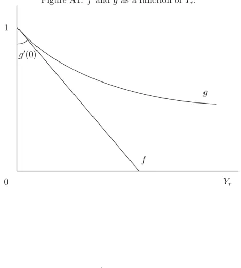
Let Yr ≡ (2αF )/Xr < 1 and g(Yr) = e−Yr. Note that (37) can then be expressed as f (Yr) =
1− Yr, which is tangent to (38) at Yr = 0:
1− Yr = g(0) + g0(0)(Yr− 0).
Since (38) is strictly convex, it lies strictly above its tangent. Put differently, f (Yr) = 1− Yr <
e−Yr = g(Y
r) holds for all Yr > 0 (see Figure A1). Hence, the right-hand side of (36) exceeds
the left-hand side of (36) at the equilibrium mass of firms nar. By uniqueness of the optimal mass of firms, and since the right-hand side of (36) exceeds the left-hand side if and only if
nr > nor, we may conclude that nar > nor, which proves our claim (see Figure A2).
[Insert Figures A1 and A2 around here]
Appendix C: Proof of Proposition 2
Conditions (6) and (7) must hold for both country-r and country-s firms at every price equi-librium which, using (2)–(4), yields
∂Πr(i) ∂pr(i) − ∂Πs(j) ∂ps(j) = 0 ⇐⇒ c · wr pr(i)− ws ps(j) ¸ = ln µ pr(i) ps(j) ¶ . (39)
19To check this, note that lim
nr→0f0(nr) = c/α > limnr→0g0(nr) = 0. The last equality is obtained as
follows. Noting that
ln g0(nr) =− 2 nr · ln(nr) 1/nr + α 2c ¸ + ln ³α c ´ +αF cL,
and that limnr→0ln nr/(1/nr) = 0 by l’Hospital’s rule, we have
lim nr→0 ln g0(nr) =− lim nr→0 2 nr× limnr→0 · ln(nr) 1/nr + α 2c ¸ + ln ³α c ´ +αF cL =−∞,
It is also readily verified that Qr(i)T Qs(j) ⇐⇒ − Lr+ Ls α ln · pr(i) ps(j) ¸ T 0. (40)
Furthermore, an equilibrium is such that firms earn zero profit, i.e.,
Πr(i) = wr ½· pr(i) wr − c ¸ Qr(i)− F ¾ = 0 Πs(j) = ws ½· ps(j) ws − c ¸ Qs(j)− F ¾ = 0.
Assume that there exists i ∈ Ωr and j ∈ Ωs such that pr(i) > ps(j). Then condition (39)
implies that wr pr(i) > ws ps(j) =⇒ pr(i) wr < ps(j) ws ,
whereas condition (40) implies that Qr(i) < Qs(j). Hence, Πr(i) < Πs(j), which is incompatible
with an equilibrium. We may hence conclude that pr(i) = ps(j) must hold for all i∈ Ωr and
j ∈ Ωs, which shows that product prices are equalized. Condition (39) then shows that wr = ws,
Figure 1: N/No as a function of L. 0 10 20 30 40 50 1.0 1.1 1.2 1.3 1.4 L N N o
Figure 2: U/Uo as a function of L.
0 10 20 30 40 50 0.6 0.7 0.8 0.9 1.0 L U U o
Figure A1: f and g as a function of Yr. Yr 1 f g 0 g0(0)
Figure A2: Excess entry.
n 0 no r nar 1 f g g(na r) f (nar)