An Empirically-Based Taxonomy of Dutch Manufacturing: Innovation Policy Implications

Texte intégral

(1)2004s-36. An Empirically-Based Taxonomy of Dutch Manufacturing: Innovation Policy Implications Wladimir Raymond, Pierre Mohnen, Franz Palm, Sybrand Schim van der Loeff. Série Scientifique Scientific Series. Montréal Juin 2004. © 2004 Wladimir Raymond, Pierre Mohnen, Franz Palm, Sybrand Schim van der Loeff. Tous droits réservés. All rights reserved. Reproduction partielle permise avec citation du document source, incluant la notice ©. Short sections may be quoted without explicit permission, if full credit, including © notice, is given to the source..

(2) CIRANO Le CIRANO est un organisme sans but lucratif constitué en vertu de la Loi des compagnies du Québec. Le financement de son infrastructure et de ses activités de recherche provient des cotisations de ses organisations-membres, d’une subvention d’infrastructure du ministère de la Recherche, de la Science et de la Technologie, de même que des subventions et mandats obtenus par ses équipes de recherche. CIRANO is a private non-profit organization incorporated under the Québec Companies Act. Its infrastructure and research activities are funded through fees paid by member organizations, an infrastructure grant from the Ministère de la Recherche, de la Science et de la Technologie, and grants and research mandates obtained by its research teams. Les organisations-partenaires / The Partner Organizations PARTENAIRE MAJEUR . Ministère du développement économique et régional et de la recherche [MDERR] PARTENAIRES . Alcan inc. . Axa Canada . Banque du Canada . Banque Laurentienne du Canada . Banque Nationale du Canada . Banque Royale du Canada . Bell Canada . BMO Groupe Financier . Bombardier . Bourse de Montréal . Caisse de dépôt et placement du Québec . Développement des ressources humaines Canada [DRHC] . Fédération des caisses Desjardins du Québec . GazMétro . Hydro-Québec . Industrie Canada . Ministère des Finances du Québec . Pratt & Whitney Canada Inc. . Raymond Chabot Grant Thornton . Ville de Montréal . École Polytechnique de Montréal . HEC Montréal . Université Concordia . Université de Montréal . Université du Québec à Montréal . Université Laval . Université McGill . Université de Sherbrooke ASSOCIE A : . Institut de Finance Mathématique de Montréal (IFM2) . Laboratoires universitaires Bell Canada . Réseau de calcul et de modélisation mathématique [RCM2] . Réseau de centres d’excellence MITACS (Les mathématiques des technologies de l’information et des systèmes complexes) Les cahiers de la série scientifique (CS) visent à rendre accessibles des résultats de recherche effectuée au CIRANO afin de susciter échanges et commentaires. Ces cahiers sont écrits dans le style des publications scientifiques. Les idées et les opinions émises sont sous l’unique responsabilité des auteurs et ne représentent pas nécessairement les positions du CIRANO ou de ses partenaires. This paper presents research carried out at CIRANO and aims at encouraging discussion and comment. The observations and viewpoints expressed are the sole responsibility of the authors. They do not necessarily represent positions of CIRANO or its partners.. ISSN 1198-8177.

(3) An Empirically-Based Taxonomy of Dutch Manufacturing: Innovation Policy Implications* Wladimir Raymond†, Pierre Mohnen‡, Franz Palm§, Sybrand Schim van der Loeff** Résumé / Abstract Dans cette étude, nous examinons empiriquement dans quelle mesure le comportement innovateur est homogène dans les entreprises néerlandaises, afin d'établir une classification industrielle du secteur manufacturier des Pays-Bas, qui puisse servir à mettre en place une politique d'innovation. Nous utilisons un modèle tobit à double censure qui explique à la fois la décision d'innover et l'intensité d'innovation des firmes innovantes. Le modèle est estimé pour onze industries définies suivant la classification industrielle type néerlandaise (SBI 1993). À partir d'un test de rapport de vraisemblance sur l'égalité des paramètres, nous arrivons à cerner trois groupes d'industries qui se ressemblent dans leur comportement innovateur: un groupe high-tech, un groupe low-tech et les entreprises du secteur du bois. La même classification ressort des enquêtes communautaires d'innovation CIS 2, CIS 2.5 et CIS 3 des Pays-Bas. Mots clés : enquête communautaire d'innovation, classification industrielle, politique d'innovation, modèle tobit à double censure. The paper studies the degree of homogeneity of innovative behavior in order to determine empirically an industry classification of Dutch manufacturing that can be used for policy purposes. We use a twolimit tobit model with sample selection, which explains the decisions by business enterprises to innovate and the impact these decisions have on the share of innovative sales. The model is estimated for eleven industries based on the Dutch Standard Industrial Classification (SBI 1993). A likelihood ratio test (LR) is then performed to test for equality of the parameters across industries. We find that Dutch manufacturing consists of three groups of industries in terms of innovative behavior, a hightech group, a low-tech group and the industry of wood, where firms seem to have a rather different innovative behavior from the remaining industries. The same pattern shows up in the three Dutch Community Innovation Surveys. Keywords: generalized tobit, high-tech industry, homogeneity, innovation policy, likelihood ratio test, model of friction, sample selection, two-limit tobit model, TPP innovator. Codes JEL : C34, C51, O33, O38 *. The empirical part of this study has been carried out at the Centre for Research of Economic Microdata at Statistics Netherlands. The authors wish to thank Statistics Netherlands, and in particular Bert Diederen, for helping us in accessing and using the Micronoom data set. The views expressed in this paper are solely those of the authors. The authors also wish to thank François Laisney, Patrick Waelbroek and participants at presentations in Maastricht, Strasbourg, Leuven and Lille for their helpful comments. The first author acknowledges financial support from METEOR. † University of Maastricht, P.O. Box 616 6200 MD Maastricht, The Netherlands W.Raymond@KE.unimaas.nl ‡ University of Maastricht, MERIT and CIRANO; P.Mohnen@MERIT.unimaas.nl § University of Maastricht and CESifo fellow, F.Palm@KE.unimaas.nl ** University of Maastricht, S.Loeff@KE.unimaas.nl.

(4) 1. Introduction. Industry classification is of great importance for innovation policy. In order to encourage R&D or innovation, governments are interested in targeting their support towards certain types of firms or industries. It is easier to work with a few well-defined industries than with a multitude of heterogeneous firms. But these industries should be as homogeneous as possible. Therefore, in order to avoid misclassification costs, industries have to be classified as accurately as possible. The objective of this paper is to study the degree of homogeneity of innovative behavior in order to determine empirically an industry classification of Dutch manufacturing that can be used for policy purposes. Two well-known and frequently used taxonomies are the Pavitt (1984) and the Organization for Economic Cooperation and Development (OECD (1999)) industry classifications. Using data on about 2000 significant innovations in Britain from 1945-79, Pavitt (1984) derives a classification where three categories of innovating firms are identified: supplier-dominated, production intensive, and science-based. The OECD uses the ratio of R&D expenditures over gross output as an indicator to classify manufacturing industries of the OECD countries in the categories of high-technology, medium-high-technology, medium-low-technology and low-technology. In contrast, Baldwin and Gellatly (2000) argue against the use of too rigid industry classifications. They perform a principal component analysis (PCA) on different innovation indicators on new technology based firms in Canada. They find that industry classification is highly sensitive to the choice of the underlying indicators, and that high-technology firms can be found in the industries that are commonly labeled low-technology and vice versa. The above classifications all suffer from the absence of a model of innovative behavior. The OECD classification relies on a single indicator, and is therefore too incomplete to be useful for innovation policies. The PCA approach is firmbased, therefore, unless very detailed information at the firm level is available to the policy maker, innovation policies based on this approach are almost impossible. The Pavitt classification, which is the most useful for innovation policies, is constructed more on a priori knowledge and assumptions about industry characteristics and interrelationships than on empirical findings regarding their innovative behavior. Like the OECD classification and the PCA approach, the Pavitt classification is essentially descriptive. He even reports regressions results that contradict his theory. The main contribution of our study is that we use, to set up an industry classification, an econometric model that explains the decisions by business enterprises in Dutch manufacturing to innovate and the impact of these decisions on the share of innovative sales. Our model belongs to the class of the generalized tobit models used among others by Crépon et al. (1996), Felder et al. (1996), Brouwer and Kleinknecht (1996), Mohnen and Dagenais (2001), and Mairesse and Mohnen (2001) to explain innovation performance in the presence of censored data.1 It combines the two-limit tobit and the generalized tobit models. In order to study homogeneity among the manufacturing industries, we shall estimate the model for each industry as described in Appendix A. Then, we shall estimate the model for categories formed 1 The first two studies use a generalized tobit model to study the determinants of innovation input (as measured by R&D or total innovation expenditures) while the other three study the determinants of innovation output (as measured by the share of innovative sales in total sales).. 2.

(5) by grouping industries, and test whether industries included in a category are similar in terms of innovative behavior. A category is called homogeneous if the parameters of the model for each industry in that category are identical. To implement our model, we use firm-level data stemming from three Dutch Community Innovation Surveys (CIS) pertaining to the periods 1994-96, 199698 and 1998-2000, and merged with production (PS) and finance (SFO) survey data for the periods 1996, 1998 and 2000. The paper is organized as follows. Section 2 describes existing taxonomies and implications for innovation policies. The model and the likelihood ratio (LR) test are explained in Section 3. In Section 4 we describe the data sources, the variables constructed from the data samples, and some descriptive statistics. Empirical results for the model and the industry classification resulting from the LR test, and its policy implications are presented and discussed in Section 5. In Section 6 we summarize and conclude.. 2. Existing taxonomies and innovation policy. In the literature on technical change, existing taxonomies are often driven by the need to identify technology-intensive industries. Indeed, firms that belong to these industries behave differently: they tend to innovate more, conquer new markets, use available resources more efficiently and offer higher remuneration to their employees. It is also admitted that, in the knowledge-based economy, innovation is the key to firms’ performance in terms of survival and productivity. Thus, the characteristics and the innovative behavior of an industry are important to innovation policy makers. In order to encourage innovation, they try to allocate, as efficiently as possible, resources to these industries. As a consequence, a misclassification of industries can have important social costs resulting from a suboptimal allocation of resources. In this section some existing taxonomies and the implications for innovation policies are explained.. 2.1. The Organization for Economic Cooperation and Development (OECD) classification. There are two OECD industry classifications. In the first one, the OECD uses the direct R&D intensity expressed as the ratio of R&D expenditures over gross output or over value-added. The first classification consists of three categories of industries, namely the high-technology, the medium-technology, and the lowtechnology industries. This classification has several drawbacks, for instance, it is not stable across the two measures used for R&D intensity.2 The revised indicator is the overall R&D intensity, which is the intensity of an indirect R&D. This latter measure is defined as the ratio of R&D expenditures plus technology embodied in intermediate and capital goods over gross output. The revised classification, which is currently used, consists of four categories of industries: the high-technology, the medium-high-technology, the medium-low-technology and the low-technology industries.3 The OECD taxonomy is based on one single innovation-input indicator, namely the R&D intensity. R&D is an important input to the innovation pro2 See. Hatzichronoglou (1997) for more details. that belong to these categories are described in details in OECD (1999).. 3 Industries. 3.

(6) cess. Calvert et al. (1996) find that, for the European countries included in their analysis, enterprises with the highest R&D intensities have the highest returns to innovation as measured by the percentages of sales from new or improved products. Nevertheless, R&D is not the only important innovation-input indicator to innovation, and there are many other innovation policy instruments besides R&D support. For instance, a few of the wide-ranging policy reforms suggested by the OECD (1998) are ‘improving the efficiency and the leverage of industrial R&D support’, or ‘strengthening technology diffusion mechanisms by encouraging more competition in product markets’. Thus, the OECD taxonomy, because of its unidimensional feature, is not suitable for innovation policies and ignores various other facets of the innovation process.. 2.2. A principal component analysis approach (PCA). Baldwin and Gellatly (2000) use data from The Survey of Operating and Financing Practices provided by Statistics Canada for their classification. The population of interest in their study is the population of small new technologybased firms (NTBFs) that entered the commercial sector (both goods and services) during the period 1983-86, and survived to 1993. They state that, in existing taxonomies (such as the OECD taxonomy), small firms are underrepresented, since the aggregate measures at the industry level are often determined by large firms. They also point out that existing industry taxonomies have a unidimensional characteristic and are therefore too narrow and incomplete. To set up their classification, they perform a principal component analysis (PCA) by accounting for innovation indicators, such as worker skills and technology use, that are commonly used to classify industries. Their framework constitutes a multidimensional approach to industry classification, and reveals two findings: first, industry classifications are highly sensitive to the indicators that are used to construct them; and high-technology firms are found in many industries, especially in the ones that are labeled low-technology. Policy implications depend strongly on the characteristics of the PCA approach to industry classification. As seen earlier, the PCA framework has a multidimensional feature. ‘High-tech’ firms may focus on developing innovations, e.g. by introducing new or improved products onto the market, integrating existing technologies into current production methods (technology use), or investing in improving worker skills (human capital development). These three activities may be disparate and, therefore, ‘high-tech’ firms may have different objectives. As a result, any innovation policy should account for these three objectives. The multidimensional facet of the PCA framework implies multidimensionally faceted innovation policies. Another motivation of the authors is to deal with the underrepresentation of small firms, when industry aggregates are used to classify industries. Small new technology-based firms (NTBFs) are often ignored by policy makers. They suggest that, in the future, such firms should be given great considerations in innovation policies, as they are ‘...spearheading the new technological revolution in many industries’. Finally, as we saw earlier, one of the findings of the authors is that hightech firms may be found in low-tech industries and vice versa. That means industries consist of heterogeneous firms, as opposed to the assumption of homogeneity underlying industry classifications. Thus, a large number of firms 4.

(7) may be penalized when innovation policies are carried out at the industry level. Such firms are advanced firms that belong to the low-tech industries. These firms are ‘often more sophisticated,..., than ‘average firms’ in a ‘high-tech’ sector’. Consequently, this type of firms should be treated differently from the remaining firms in the low-tech industries by policy makers. Similarly, low-tech firms belonging to the high-tech industries may be unfairly rewarded by innovation policy makers, and should be treated differently from the remaining firms in the high-tech industries. According to the PCA approach to industry classification, innovation policies may favor certain indicators of technological performance over others, but they should be discretionary, and should not view the high-tech and low-tech divide between firms or industries as schematic. Specifically, the high-tech firms that belong to the low-tech industries should be identified by innovation policy makers. However, it is a difficult task, as policies are usually carried out at the industry level. Consequently, the PCA approach to industry classification may not be very useful for innovation policies.. 2.3. The Pavitt classification. Pavitt (1984) uses data on about 2000 ‘significant innovations’ in Britain from 1945-79 for his classification. A significant innovation is qualified as such by ‘experts’, who for each sector, define the threshold of significance for an innovation. Pavitt (1984) starts from these significant innovations, identifies the innovating firms and their sectors of economic activity. He also identifies the type of the innovations (product or process innovations) according to whether or not they are produced and used in the same sector, and the sources of knowledge inputs to them (e.g. universities). On the basis of some a priori assumptions coming from previous theories and possibly supported by the data, he sets up an industry classification where similarities and differences among sectors in the sources, nature and impact of innovations, as well as in the characteristics of the innovating firms are explained. Pavitt’s classification consists of three categories, namely the ‘supplier-dominated’, the ‘production intensive’ and the ‘sciencebased’ categories. The middle category consists of two sub-categories: scale intensive and specialized-suppliers. At a two-digit level of the Minimum List Heading (MLH),4 the distribution of industries across categories is as follows: the supplier-dominated category consists of innovating firms in textiles, leather and footwear; the scale intensive sub-category of the production intensive category consists of the industries of food, metal manufacturing, shipbuilding, motor vehicles and glass and cement; the specialized-suppliers sub-category consists of the industries of mechanical engineering and instrument engineering; and the science-based category consists of innovating firms in the industries of chemicals, electrical, and electronic engineering. The first policy implication of the Pavitt classification is the relative importance of ‘science and technology push’ and ‘demand pull’ in innovative activities. Pavitt finds that in supplier-dominated and production intensive firms demand pull stimulates innovative activities. More specifically, he finds that in these categories of firms demand pull, as measured by investment activities in user industries, is likely to stimulate ‘innovative activities in both the production en4 The. MLH is the UK equivalent of the Standard Industry Classification (SIC).. 5.

(8) gineering departments of user firms, and the upstream firms supplying capital goods’. No such evidence is found for science-based firms. Another implication of his classification is the relative importance of product and process innovation. It suggests that, in product groups with a high number of science-based firms, i.e. firms with a high R&D intensity, it may be expected that a high proportion of product/market opportunities are generated outside the group products. In other words, R&D intensity influences strongly and positively product innovation (as defined by Pavitt in his study) in science-based firms. In such firms, patent intensity is expected to have a stronger influence on product innovation. Additionally, in industries with production intensive firms, Pavitt’s classification suggests that a high proportion of resources may be expected to be devoted to process innovations, and that these firms have high capital intensities, plant size and industrial concentration. Pavitt (1984) also examines the extent to which firms develop their own process innovations, or buy them from suppliers. Supplier-dominated firms, with small production plants, tend to buy innovations from suppliers. On the other hand, production intensive and science-based firms, with generally large production plants, develop in-house process innovations. In other words, the Pavitt taxonomy suggests that there is a positive relationship between the ‘proportion of a sector’s process technology generated in-house, ..., and the size of firms and production plant’.. 2.4. Aim of the study. As the OECD taxonomy relies on a single innovation input indicator, R&D intensity, it is too narrow and will be incomplete for policy purposes. R&D expenditures cannot explain by itself the complicated innovation process. Baldwin and Gellatly (2000) point out that the OECD taxonomy is likely to be biased, and therefore cannot be the basis for wide-ranging innovation policies. The PCA approach considered by Baldwin and Gellatly (2000), overcomes the problem of incompleteness by accounting for various innovation indicators that are commonly used to classify industries, leading to a multidimensional approach. Despite interesting findings from the PCA approach, it is not fully satisfactory. First, it is based on a principal component analysis, letting the data speak without an underlying model. The PCA approach is therefore essentially descriptive. Furthermore, it is not of great help in recommending innovation policies, since it is based on firm level characteristics, while policies are very often industry-based. Its main contribution is that innovation policy measures should be discretionary. The Pavitt taxonomy is the most useful of the taxonomies considered here for innovation policies. It accounts for various criteria of the innovation process to classify industries, and its policy implications are based on a ‘theory’ derived from experts opinions about industries and empirical evidence. However, the Pavitt taxonomy is based on the population of innovating firms. There is no information regarding the classification of non-innovating firms. Therefore, it provides no guidance for policy measures to encourage non-innovating firms to become innovators. Furthermore, significant innovations are defined by ‘experts’, and may therefore suffer from subjectiveness. The significant threshold fixed by the innovation experts is not necessarily the same for all sectors. Finally, Pavitt also calls his taxonomy a ‘theory’, and no formal tests of the theory 6.

(9) could take place. The resulting taxonomy is therefore dependent on the validity of the a priori assumptions and the experts’ opinions. Indeed, it is not clear that his theory is always in accordance with the facts.5 Our study proposes an empirically-based taxonomy of the Dutch manufacturing industries with a view to innovation policies. We account for various innovation (input and output) indicators and study the innovative behavior of eleven manufacturing industries. We estimate a model of the determinants of innovation and test for homogeneity among industries. A category of industries is considered as homogeneous if we cannot reject the hypothesis that the parameters of the model for all the industries included in that category are identical.. 3. The model. The model we consider in this study explains the decisions by Dutch manufacturing enterprises to innovate and the impact of these decisions on the share of innovative sales. It is derived from the literature on the determinants of innovation, and a few studies on this type using innovation survey data for the manufacturing industries of some European countries are described in Table 1. Modelling the determinants of innovation strongly depends on the design of the Community Innovation Survey. In order to correct for selection bias, tobit-type models are commonly used in empirical studies. Our model resembles the generalized tobit model studied by Crépon et al. (1996), Felder et al. (1996), Brouwer and Kleinknecht (1996), Mohnen and Dagenais (2001), and Mairesse and Mohnen (2001). It consists of two equations, a selection equation that discriminates between TPP innovators and non-innovators, and a regression equation explaining the share of innovative sales for innovators. A TPP innovator is an enterprise that has implemented new or improved products, or new or improved processes during the period under review. Formally, our model can be written as: y1∗ = β1 x1 + ε1 y2∗ = β2 x2 + ε2 , where the dependent  0    c1 y2 = y∗    2 c2. (1) (2). variable is defined as: if y1∗ ≤ 0 (non-innovators) if y1∗ > 0 and y2∗ ≤ c1 (process-only innovators) . if y1∗ > 0 and c1 < y2∗ ≤ c2 (product innovators) if y1∗ > 0 and y2∗ > c2 (large product innovators). (3). As it stands in equations (1), (2) and (3), our model is a combination of the two-limit tobit model and the generalized tobit model.6 More specifically, it is a two-limit tobit model with sample selection. It is different from the former in that it consists of two decisions (two latent variables), and from the latter in that it has two additional thresholds c1 and c2 . 5 In. an appendix, Pavitt (1984) reports regressions that contradict his theory. two-limit tobit model is described in details in Maddala (1983) and Thomas (2000). A variant of this model is the so-called model of friction used by Rosett (1959). 6 The. 7.

(10) Table 1: Empirical studies on the determinants of innovation in manufacturing using the Community Innovation Survey Country Data Def. of Heterogeneity Econometric innovator treatment technique 1. Brouwer and The Netherlands CIS 1, 1990-1992 Product innovator Dummy for highGeneralized Kleinknecht, 1996 + other data technology opportutobit nity industries‡ Study. France. French Innovation Survey, 1986-1990 + other data. Product, process, organizational, or marketing innovator. Industry dummies; sample of all manufacturing firms. Asymptotic least squares (ALS). 3. Mohnen and Dagenais, 2001. Denmark, Ireland. CIS 1, 1990-1992. Firm with innovative activities. Industry dummies; sample of all manufacturing firms. Generalized tobit. 4. Mairesse and Mohnen, 2001. France, Belgium, Denmark, Germany Ireland, Italy, The Netherlands, Norway. CIS 1, 1990-1992; CIS 2, 1994-1996. Firm with innovative activities. Sample split: highand low-R&D industries; industry dummies in both groups. Generalized tobit. 5. Janz and Peters, 2002. Germany. CIS 3, 1998-2000. Product innovator with positive innovation expenditures. Industry dummies; sample of all manufacturing firms. 3-Stage least squares (3SLS). 6. Janz et al., 2003. Germany, Sweden. CIS 3, 1998-2000. 8. 2. Crépon et al., 1998. Product innovator Industry dummies; Generalized tobit with positive innosample of R&D + 2-stage least vation expenditures intensive firms squares (2SLS) ‡ the reference is the group of low technological industries consisting of the ‘supplier-dominated’ industries of the Pavitt classification.

(11) Equation (1) The latent variable y1∗ captures the expected post-innovation return to innovation. It is a function of explanatory variables included in the vector x1 . The latent variable y1∗ pertains to both non-innovating and innovating enterprises. Because of the way the innovation survey is designed, very few explanatory variables are available for both types of enterprises.7 Besides the constant term, we have included into x1 two variables: size and relative size.8 The former is measured by the number of employees (in natural logarithms), while the latter is the ratio of an enterprise’s turnover over total industry’s turnover (in natural logarithms). According to the Schumpeterian hypotheses, size and relative size (as measured by the market share) are expected to have a positive effect on innovation activities (input side of innovation). It is often argued that larger firms have better access to finance, therefore are more likely to engage in risky projects, and benefit from economies of scale. Several recent empirical studies find evidence that size affects positively the decision by firms to invest in R&D (see Crépon et al. (1996) and Felder et al. (1996)) and the probability to be product innovators (see Brouwer and Kleinknecht (1996), Mohnen and Dagenais (2001), and Mairesse and Mohnen (2001)). When y1∗ is sufficiently large, i.e. the expected return to innovation is high enough, an enterprise has enough incentive to innovate, then the observed y1 equals one, meaning that the enterprise is a TPP innovator. Finally, ε1 is the error term that captures the effects unaccounted for by the model, and β1 is the vector of parameters to be estimated.9 Equation (2) The second equation pertains only to TPP innovating firms. Information included in x2 in addition to size is available in the CIS only for innovators. The vector x2 comprises, besides the constant term, the variables size, demand pull, technology push, subsidies, partnership, R&D intensity, continuous R&D and non-R&D performer as defined in Section 4.2. All the studies mentioned in Table 1 account for a demand pull variable according to the Schmooklerian tradition. Technology push is included in x2 on the basis of the Schumpeterian tradition. We expect enterprises that receive subsidies to be more innovative, on the grounds that they do more R&D which may also be expected to affect positively innovation output. While continuous R&D is very often found to affect positively innovation output, there is mixed evidence about the effect of developing innovation in partnership. It is often argued that, experience and knowledge accumulated from past R&D influences positively innovation output, while developing innovation in partnership is relevant only to firms lacking of knowledge (‘weak’ innovators).10 The dependent variable is the share of innovative sales in total sales. It is expressed as the ratio of sales from new or improved products over total sales. This figure is directly reported by the surveyed enterprises. As the original share of innovative sales lies within 7 See. Section 4. the innovation survey enterprises report whether they belong to a group or not. This potentially important information was, however, not available in the data provided by CBS. 9 In order to simplify the notation, the enterprise and industry subscripts have been dropped. 10 See Brouwer and Kleinknecht (1996) for details. 8 In. 9.

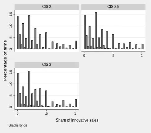
(12) the unit interval, we take the logit transformation that may take on any real value. In addition, the logit transform makes the distribution of the share of innovative sales more symmetric than the distribution in Figure 1. β2 is the vector of parameters to be estimated, and ε2 is the error term capturing the effects influencing the share of innovative sales unaccounted for by the model.. Figure 1: Histogram of the share of innovative sales for the sub-sample of innovative firms: CIS 2, CIS 2.5, and CIS 3 The Netherlands CIS 2.5. 0. 0. .5. 1. 15. CIS 3. 0. 5. 10. Percentage of firms. 5. 10. 15. CIS 2. 0. .5. 1. Share of innovative sales Graphs by cis. The thresholds c 1 and c 2 TPP innovators comprise product-only innovators, process-only innovators, and product-and-process innovators. As there is no quantitative measure for a process innovation in the CIS, process-only innovators have a zero share of innovative sales during the period under review. Therefore, the logit transform of the share of innovative sales cannot be applied to process-only innovators. Mairesse and Mohnen (2001) choose to substitute, for the zero shares of processonly innovators, the smallest positive value of the original share of innovative sales, namely 0.01. Klomp and Van Leeuwen (2001) use a similar approach where the smallest positive value of the share of innovative sales is 0.001. In our model, we choose to censor the zero values for process-only innovators, by fixing a threshold c1 and treat all the zero values as values that belong to the censored 10.

(13) region.11 The difference between our approach and that of Mairesse and Mohnen (2001), and Klomp and Van Leeuwen (2001) is that, for observations with share of innovative sales below the smallest positive value, the probability that the share is below this value has been used rather than the value of the density function evaluated at this value. The same ‘technical’ explanation holds for the category of large product innovators. In this case, values equal to unity are censored, by fixing the threshold c2 to 0.95, which is the value of the largest share less than one. Again, the probability that the share is above 0.95 has been used rather than the value of the density function evaluated at a value close to 1. A further reason to introduce the thresholds c1 and c2 is that, according to the Oslo manual, process-only innovators are to be treated differently from product innovators and non-innovators. They are not to be treated as noninnovators, given that they have implemented new or improved processes. Actually, they produce unchanged products with changed methods, as opposed to non-innovators that produce unchanged products with unchanged methods. They are different from product-innovators in the sense that they have not implemented new or improved products (during the period under review), but they might do so in the future. Finally, the category of large product innovators, as measured by the share of innovative sales, mostly consists of firms that got established during the period studied by the innovation survey. Again, according to the Oslo manual, these firms are to be treated differently, as they may be different from the remaining firms in terms of innovation activities, objectives and characteristics. Before we turn to the estimation of the model, it is to be noted that the distribution of the original share of innovative sales in total sales is rather similar in the three waves of innovation surveys included in this study. Figure 1 reveals that, innovating firms in the Dutch manufacturing during the period 1994-2000, have a rather small or medium share of innovative sales in total sales.. 3.1. Estimation. In order to estimate the model, for each industry, the error terms are assumed to follow µ a bivariate ¶ normal distribution with zero mean and covariance matrix 1 ρσ Σ= , where ρ and σ are the correlation between the error terms ρσ σ 2 and the standard deviation of ε2 respectively. The model is estimated by the method of maximum likelihood, and the log-likelihood function is given by: 12 11 For 12 See. the estimation, logit transforms of the thresholds c1 and c2 have been used. Appendix B for the derivation of this likelihood function.. 11.

(14) X. ln L =. ln Φ1 (−β1 x1 ). 0. +. X c1. . . ln. ln Φ1 . ³. c1 1−c1. ´. − β 2 x2. σ. . .  − Φ2 −β1 x1 ,. ln. ³. c1 1−c1. ´. σ. − β 2 x2. . , ρ . (4) h ³ ´ i  y2 β1 x 1 + ln ln 1−y2 − β2 x2 − β 2 x2 X 1  × Φ1   p ln  φ1  + 2) σ σ (1 − ρ ∗ y2 ´ ´ ³     ³  c2 c2 − β x − β x ln ln 1−c X 2 2 2 2 1−c2 2  + Φ2 −β1 x1 , , ρ  , + ln 1 − Φ1 (−β1 x1 ) − Φ1  σ σ c . . ³. y2 1−y2. ´. . . ρ σ. 2. where Φ1 and φ1 are the univariate standard normal cumulative distribution and density functions, and Φ2 is the bivariate standard normal cumulative distribution.13 Furthermore, we assume the vectors of disturbances to be independent across industries such that, the log-likelihood function for the Dutch manufacturing sector is the sum of the log-likelihood functions for each industry in this sector. The disturbance covariance matrix Σ is allowed to be different across industries. A likelihood ratio (LR) test for homogeneity among industries. All the empirical studies on the determinants of innovation mentioned in Table 1 implicitly assume that all industries in manufacturing have the same innovative behavior (in terms of the parameters of the model) and different intercepts. The only exception is the study by Mairesse and Mohnen (2001) that assumes that firms in the high-R&D industries have a different innovative behavior from firms in the low-R&D industries. However, the authors do not test this difference in innovative behavior. In our study, we account for the difference in innovative behavior across industries by estimating our model for each of the eleven Dutch manufacturing industries as described in Appendix A. We shall be referring to this as the unrestricted model. Let a category, for instance, consist of k industries. The null hypothesis is that the p parameters of the model, i.e. the slope parameters, the two intercepts and the parameters ρ and σ, for each of the k industries are equal versus the alternative that at least for one industry a parameter is different from the corresponding parameters of the k − 1 other industries. The resulting test statistic must be compared to the critical value for a χ2 distribution with (k − 1)p degrees of freedom. In the case that we allow the two intercepts in the k industries to differ, the number of degrees of freedom is (k − 1)(p − 2).. 4. Data. The data used to implement the model are collected by the Centraal Bureau voor de Statistiek (CBS). They stem from three waves of the Dutch Community ³ ´ ³ ´ ³ ´ y2 c1 c2 expressions ln 1−c , ln 1−c and ln 1−y are the logit transforms of the 1 2 2 thresholds and the original share of innovative sales respectively. 13 The. 12.

(15) Innovation Survey, CIS 2, 2.5 and 3, merged with data from production and finance surveys (respectively PS and SFO). Only enterprises in Dutch manufacturing (SBI 15-37) are included in the analysis. The population of interest consists of enterprises with at least ten employees and a positive turnover at the end of the period covered by the innovation survey. The Community Innovation Survey data are collected at the enterprise level. A combination of a census and a stratified random sampling is used. A census is used for the population of large enterprises, and a stratified random sampling is used for small- and medium-size enterprises. The size of an enterprise is measured by the number of employees, and the stratum variables are the economic activity and the size of an enterprise, where the economic activity is given by the Dutch standard industrial classification (SBI 1993).14 Finally, the cut-off point used by CBS to choose between a census and a sampling is 100 employees. Like in the CIS, the statistical unit of analysis within the Production Survey is the enterprise. A census is also used for large enterprises, and a stratified random sampling for small- and medium-size enterprises. The stratum variables and the cut-off points are the same as in the CIS. However, unlike the CIS, non-financial activities are not covered by the PS, implying that enterprises in the institutions of finance, insurance and pension funds (SBI 65-67) are not surveyed. The PS data included in this study replace the CIS equivalents and pertain to the periods 1996, 1998 and 2000. The corresponding CIS data have been removed from the CIS data base. Finally, unlike the two surveys mentioned above, the statistical unit within the SFO is the ‘group of enterprises’. A group of enterprises (which we refer to as ‘company’) results from consolidating the activities of a collection of legally connected enterprises. The SFO, which consists of the SFGO (Finance Statistics for Large Companies) and the SFKO (Finance Statistics for Small Companies), 15 collects detailed information on balance sheet and income statement items for the population of non-financial companies established in the Netherlands. 16 As a result, data for companies whose ultimate benefit owners are Dutch, but are established abroad, are not available in the SFO. Additionally, like in the PS, enterprises in the institutions of finance, insurance and pension funds are not included in the consolidation of companies’ finances. Finally, the SFO data included in this study pertain to the same periods as for the PS, namely 1996, 1998 and 2000. They are used to replace financial variables that have been removed from the CIS data bank by CBS. We explain now the construction of the variables included in this analysis.. 4.1. Dependent variables. The variables of interest in this study are the incidence and the magnitude of innovation. In the innovation survey, an enterprise is asked whether or not it has implemented at least one new or improved product, and whether or not it has implemented at least one new or improved process during the period under re14 See. Appendix A. company is deemed to be large if its balance sheet is larger than a certain threshold. In the Netherlands, from 1977 until 1994, this threshold was 10 million guilders. From 1995 on, it became 25 million guilders. 16 The ultimate benefit owner (UBO) may be Dutch or foreign. 15 A. 13.

(16) view. The variable capturing the success of innovation is then constructed by assigning the value one if at least one of the questions is answered affirmatively. An enterprise having ongoing or abandoned innovative projects (without any successfully achieved innovative projects) is considered as a non-innovator for the time period under consideration. The CIS questionnaire provides information regarding the share of innovative sales in total sales. This is the measure for the success of product innovation used in this study. A logit transformation of this measure is used for reasons mentioned earlier in the analysis. A non-TPP innovator has automatically a zero innovation output intensity. Because there is no quantitative measure of the success of process innovations in the innovation survey, some TPP innovators also have a zero innovation output intensity. They are labeled as process-only innovators.17. 4.2. Explanatory variables. The explanatory variables can be classified into three categories: the enterprise characteristics, the enterprise activities and the industry characteristics. In the paragraphs below, we explain whether they are nominal or continuous, and whether they are constructed or directly extracted from one of the data sources mentioned earlier. 4.2.1. Enterprise characteristics. Size The size of an enterprise used in this study is measured by the number of employees. This variable stems from the PS and is log-transformed. Relative size This figure, defined as the ratio of the turnover of an enterprise over the turnover of the industry that the enterprise belongs to, is constructed from the original turnover of an enterprise provided by the SFO data base. A logtransformation of this ratio is used. Demand pull In the CIS questionnaire, an enterprise is asked about the importance of the objectives of innovation, ‘open-up new markets’, ‘extend product range’ and ‘replace products phased out’, on the basis of a 0-3 Likert scale. A dummy variable proxying demand pull equals one for an enterprise if at least one of the above objectives of innovation is given the highest mark (i.e. very important), and zero otherwise. Technology push 17 In fact enterprises that report to have implemented at least one new or improved product but report a zero value for the share of innovative sales in total sales are considered as nonproduct innovators in the analysis.. 14.

(17) Other innovation indicators available in the CIS are the sources of innovation. They may be internal (from the enterprise or other enterprises within the enterprise group), from the market (e.g. clients or customers), from public or private institutions (e.g. universities) or from other locations. Technology push is proxied by a dummy variable constructed from the indicators stating the importance of the sources of innovation from public or private institutions. This proxy takes on the value one if at least one of these institutions are deemed to be important or very important to an enterprise (i.e. at least one of the sources of innovation stemming from public or private institutes is given the values 2 or 3), and zero otherwise. Subsidy If an enterprise answers that it has been granted at least a subsidy during the period under review, the variable ‘subsidy’ takes on the value one and zero otherwise. Cooperation The dummy variable ‘cooperation’ takes on the value one if the enterprise reports that it undertook its innovative activities in cooperation of any kind and zero otherwise. 4.2.2. Enterprise activities. R&D intensity R&D intensity is the ratio of total (intramural and extramural) R&D expenditures (from the CIS) over total sales (from the SFO). The logarithmic transform of this variable is used when the variable takes on a positive value. Continuous R&D The dummy variable ‘continuous R&D’ takes on the value one if the enterprise reports that it performed intramural R&D continuously during the period under review and zero otherwise. Non-R&D performer The dummy variable ‘non-R&D performer’ takes on the value one if the enterprise had no (intramural or extramural) R&D expenditures during the period under review and zero otherwise.18 4.2.3. Industry characteristics. The only industry characteristics available in the CIS and included in this study are the industry dummy variables. The manufacturing industries are defined according to a two-digit classification of the SBI 1993. 18 In addition to the variable ‘R&D intensity’, the dummy variable ‘non-R&D performer’ is included in the analysis to ‘compensate’ for the fact that the log transform of the original R&D intensity is set up to zero for observations with original R&D intensity equal to zero.. 15.

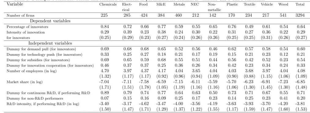
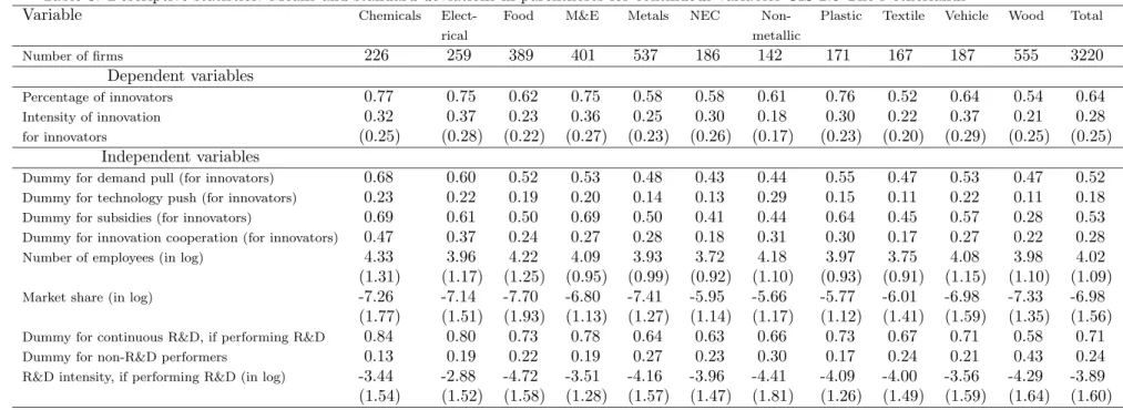
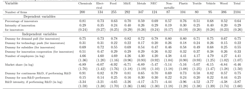
(18) 4.3. Descriptive statistics. Tables 2, 3 and 4 of descriptive statistics show that, on average, the characteristics and the activities of the enterprises in Dutch manufacturing are rather similar in the three waves of the CIS. The ‘Total’ columns reveal that, during the three periods studied by the three innovation surveys, 64 per cent of the Dutch manufacturing enterprises are TPP innovators. Furthermore, the innovative sales of the Dutch manufacturing innovators account for about 29 per cent of their total sales during the three periods. A little over half of the Dutch manufacturing innovators are granted a subsidy, roughly one third work in partnership, and about 20 per cent consider that innovation sources from public and private institutions are important or very important (technology push) during the three periods. Also, among the TPP innovators, more than 75 per cent are R&D performers and the average amounts of R&D expenditures expressed as intensities are very similar for the three periods. Finally, the percentage of continuous R&D performers is rather similar, around 75 per cent, during the three periods. The only variables that vary from one wave to another are demand pull, size and relative size as measured by the market share. The values of these variables show a decrease from CIS 2 to CIS 2.5 and an increase in CIS 3. It should be noticed that, for the three CIS, the enterprises in the industry of wood and paper (column ‘wood’) seem to be rather different from the enterprises in the manufacturing industries. These differences are particularly pronounced for the dependent variables, the variables pertaining to the firm activities and the variable subsidy. 54 per cent of the enterprises in the industry of wood are innovators while there are 64 per cent of such enterprises in the manufacturing sector as a whole. Moreover, the average return to innovation for TPP innovators of the enterprises in the industry of wood is much lower than the average return of the enterprises in total manufacturing. One explanation for this is that the industry of wood consists of a high percentage of processonly innovators. The percentage of TPP innovators in the industry of wood that are granted a subsidy is roughly 30 per cent while this percentage is more than 50 per cent in total manufacturing. Finally, looking at the variables of the enterprise activities, we notice that in the industry of wood, the percentage of R&D performers among TPP innovators, the percentage of continuous R&D performers among R&D performers and the actual average amount of R&D expenditures expressed as intensities are rather different from the equivalent figures for the manufacturing sector as a whole. From the innovation indicators presented in Tables 2, 3 and 4, a tentative conclusion can be drawn with regard to the grouping of the industries (excluding the industry of wood). For one group, containing the manufacturing of chemicals, electrical products, plastic, and machinery and equipment, the indicators of innovation input and output and the subsidy indicator take on higher than average values. These indicators take on lower than average values in a second group containing the manufacturing of food, metallic and non-metallic products, textiles, and products not elsewhere classified. In the following section it will be investigated empirically whether this grouping is purely descriptive or whether this grouping is the result of similar behavior described by an econometric model.. 16.

(19) Table 2: Descriptive statistics: Means and standard deviations in parentheses for continuous variables CIS 2 The Netherlands Variable Chemicals ElectFood M&E Metals NEC NonPlastic Textile Vehicle rical Number of firms. Wood. Total. metallic. 225. 285. 424. 384. 460. 212. 142. 170. 234. 217. 541. 3294. 0.84 0.29 (0.25). 0.72 0.39 (0.29). 0.66 0.23 (0.23). 0.77 0.38 (0.27). 0.59 0.24 (0.24). 0.55 0.30 (0.26). 0.65 0.22 (0.26). 0.76 0.31 (0.25). 0.49 0.27 (0.25). 0.61 0.36 (0.31). 0.54 0.22 (0.26). 0.64 0.29 (0.27). 0.69 0.33 0.69 0.46 4.70 (1.32) -7.04 (1.71) 0.89 0.07 -3.40 (1.50). 0.68 0.25 0.65 0.37 3.97 (1.17) -7.11 (1.51) 0.79 0.15 -3.17 (1.47). 0.68 0.27 0.59 0.37 4.37 (1.17) -7.58 (1.78) 0.74 0.16 -4.62 (1.71). 0.65 0.18 0.68 0.25 4.17 (0.92) -6.59 (1.05) 0.77 0.09 -3.47 (1.29). 0.52 0.21 0.55 0.36 4.04 (0.96) -7.15 (1.19) 0.64 0.25 -4.00 (1.37). 0.56 0.17 0.51 0.26 3.65 (0.94) -6.11 (1.16) 0.63 0.17 -3.56 (1.22). 0.46 0.19 0.44 0.34 4.04 (1.09) -5.59 (1.16) 0.50 0.23 -4.19 (1.55). 0.62 0.15 0.56 0.42 4.03 (0.90) -5.70 (1.06) 0.73 0.14 -3.63 (1.17). 0.57 0.21 0.42 0.23 3.68 (0.88) -6.23 (1.30) 0.71 0.25 -3.93 (1.59). 0.58 0.23 0.52 0.34 3.97 (1.15) -6.91 (1.45) 0.67 0.23 -3.70 (1.47). 0.54 0.12 0.23 0.24 4.04 (1.06) -7.23 (1.30) 0.55 0.41 -4.20 (1.60). 0.60 0.21 0.54 0.33 4.08 (1.09) -6.85 (1.48) 0.71 0.20 -3.81 (1.53). Dependent variables Percentage of innovators Intensity of innovation for innovators. Independent variables 17. Dummy for demand pull (for innovators) Dummy for technology push (for innovators) Dummy for subsidies (for innovators) Dummy for innovation cooperation (for innovators) Number of employees (in log) Market share (in log) Dummy for continuous R&D, if performing R&D Dummy for non-R&D performers R&D intensity, if performing R&D (in log).

(20) Table 3: Descriptive statistics: Means and standard deviations in parentheses for continuous variables CIS 2.5 The Netherlands Variable Chemicals ElectFood M&E Metals NEC NonPlastic Textile Vehicle rical Number of firms. Wood. Total. metallic. 226. 259. 389. 401. 537. 186. 142. 171. 167. 187. 555. 3220. 0.77 0.32 (0.25). 0.75 0.37 (0.28). 0.62 0.23 (0.22). 0.75 0.36 (0.27). 0.58 0.25 (0.23). 0.58 0.30 (0.26). 0.61 0.18 (0.17). 0.76 0.30 (0.23). 0.52 0.22 (0.20). 0.64 0.37 (0.29). 0.54 0.21 (0.25). 0.64 0.28 (0.25). 0.68 0.23 0.69 0.47 4.33 (1.31) -7.26 (1.77) 0.84 0.13 -3.44 (1.54). 0.60 0.22 0.61 0.37 3.96 (1.17) -7.14 (1.51) 0.80 0.19 -2.88 (1.52). 0.52 0.19 0.50 0.24 4.22 (1.25) -7.70 (1.93) 0.73 0.22 -4.72 (1.58). 0.53 0.20 0.69 0.27 4.09 (0.95) -6.80 (1.13) 0.78 0.19 -3.51 (1.28). 0.48 0.14 0.50 0.28 3.93 (0.99) -7.41 (1.27) 0.64 0.27 -4.16 (1.57). 0.43 0.13 0.41 0.18 3.72 (0.92) -5.95 (1.14) 0.63 0.23 -3.96 (1.47). 0.44 0.29 0.44 0.31 4.18 (1.10) -5.66 (1.17) 0.66 0.30 -4.41 (1.81). 0.55 0.15 0.64 0.30 3.97 (0.93) -5.77 (1.12) 0.73 0.17 -4.09 (1.26). 0.47 0.11 0.45 0.17 3.75 (0.91) -6.01 (1.41) 0.67 0.24 -4.00 (1.49). 0.53 0.22 0.57 0.27 4.08 (1.15) -6.98 (1.59) 0.71 0.21 -3.56 (1.59). 0.47 0.11 0.28 0.22 3.98 (1.10) -7.33 (1.35) 0.58 0.43 -4.29 (1.64). 0.52 0.18 0.53 0.28 4.02 (1.09) -6.98 (1.56) 0.71 0.24 -3.89 (1.60). Dependent variables Percentage of innovators Intensity of innovation for innovators. Independent variables 18. Dummy for demand pull (for innovators) Dummy for technology push (for innovators) Dummy for subsidies (for innovators) Dummy for innovation cooperation (for innovators) Number of employees (in log) Market share (in log) Dummy for continuous R&D, if performing R&D Dummy for non-R&D performers R&D intensity, if performing R&D (in log).

(21) Table 4: Descriptive statistics: Means and standard deviations in parentheses for continuous variables CIS 3 The Netherlands Variable Chemicals ElectFood M&E Metals NEC NonPlastic Textile Vehicle rical Number of firms. Wood. Total. metallic. 200. 134. 255. 292. 347. 124. 87. 104. 80. 95. 386. 2104. 0.81 0.29 (0.24). 0.73 0.35 (0.27). 0.63 0.24 (0.25). 0.70 0.40 (0.29). 0.59 0.26 (0.26). 0.69 0.29 (0.24). 0.57 0.19 (0.17). 0.76 0.30 (0.19). 0.51 0.25 (0.20). 0.68 0.40 (0.28). 0.52 0.20 (0.23). 0.64 0.29 (0.26). 0.75 0.31 0.69 0.51 4.66 (1.36) -6.89 (1.70) 0.91 0.15 -3.34 (1.59). 0.73 0.31 0.72 0.47 4.60 (1.20) -6.07 (1.42) 0.82 0.14 -3.21 (1.38). 0.78 0.22 0.55 0.29 4.69 (1.16) -6.92 (1.76) 0.79 0.25 -4.65 (1.70). 0.82 0.22 0.69 0.29 4.26 (0.96) -6.71 (1.18) 0.81 0.16 -3.26 (1.36). 0.72 0.17 0.54 0.29 4.30 (0.93) -6.89 (1.19) 0.65 0.30 -4.17 (1.66). 0.78 0.20 0.47 0.26 4.20 (0.92) -5.47 (1.10) 0.70 0.30 -3.71 (1.30). 0.80 0.26 0.46 0.32 4.38 (1.04) -5.14 (1.18) 0.69 0.22 -4.44 (1.18). 0.80 0.18 0.58 0.32 4.41 (0.90) -5.16 (1.08) 0.73 0.24 -3.96 (1.28). 0.71 0.24 0.49 0.37 4.17 (0.93) -5.07 (1.25) 0.58 0.20 -4.52 (1.38). 0.75 0.26 0.68 0.38 4.79 (1.25) -6.15 (1.47) 0.82 0.22 -3.77 (1.39). 0.67 0.15 0.25 0.26 4.27 (1.02) -6.84 (1.28) 0.57 0.44 -4.38 (1.74). 0.75 0.22 0.55 0.33 4.41 (1.07) -6.46 (1.50) 0.75 0.25 -3.87 (1.60). Dependent variables Percentage of innovators Intensity of innovation for innovators. Independent variables 19. Dummy for demand pull (for innovators) Dummy for technology push (for innovators) Dummy for subsidies (for innovators) Dummy for innovation cooperation (for innovators) Number of employees (in log) Market share (in log) Dummy for continuous R&D, if performing R&D Dummy for non-R&D performers R&D intensity, if performing R&D (in log).

(22) 5. Empirical results. This section discusses empirical results derived from our model. Our industry taxonomy stems from likelihood ratio tests performed on our model. The characteristics of the different categories in the classification are explained. We also present possible implications for innovation policies on the basis of the parameters of the model for each category. Table 5: Likelihood ratio test results for the two-limit tobit model with sample selection: CIS 2 The Netherlands Model Number of firms Log-likelihood Number of parameters Unrestricted model Chemicals 225 -482.38 14 Electrical 285 -579.37 14 M&E 384 -761.74 14 Plastic 170 -344.98 14 Vehicle 217 -429.35 14 Food 424 -845.27 14 Metals 460 -892.06 14 Non-metallic 142 -285.00 14 NEC 212 -374.76 14 Textile 234 -408.92 14 Wood 541 -1001.42 14 Restricted model 1 High-tech industry 1281 -2625.41 22 Low-tech industry 1472 -2831.79 22 Wood 541 -1001.42 14 χ2 (96) = 106.72 Restricted model 2 High-tech industry Low-tech industry. 1281 2013. -2625.41 -3861.69. χ2 (108) = 163.68 Restricted model 3 High-tech industry Low-tech industry. 1822 1472. 22 24. p − value = 0.000 -3716.48 -2831.79. χ2 (108) = 286.03. 5.1. p − value = 0.214. 24 22. p − value = 0.000. An econometrically-based industry classification. Tables 5, 6 and 7 report the relevant statistics to perform the likelihood ratio test. The model is estimated separately for eleven industries as described in Appendix A. The unrestricted model consists of eleven sub-models, where the log-likelihood is the sum of the eleven log-likelihoods of the sub-models. The restricted model assumes that the parameters are identical for industries within each category (allowing for different industry dummies), and different. 20.

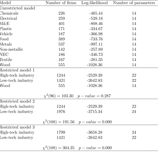
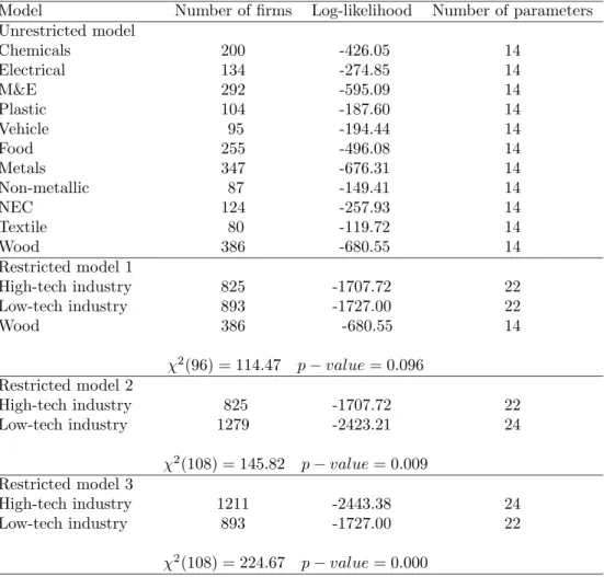
(23) Table 6: Likelihood ratio test results for the two-limit tobit model with sample selection: CIS 2.5 The Netherlands Model Number of firms Log-likelihood Number of parameters Unrestricted model Chemicals 226 -465.44 14 Electrical 259 -528.18 14 M&E 401 -808.46 14 Plastic 171 -334.67 14 Vehicle 187 -366.98 14 Food 389 -733.76 14 Metals 537 -997.11 14 Non-metallic 142 -257.89 14 NEC 186 -346.73 14 Textile 167 -281.35 14 Wood 555 -1028.36 14 Restricted model 1 High-tech industry 1244 -2529.39 22 Low-tech industry 1421 -2642.83 22 Wood 555 -1028.36 14 χ2 (96) = 103.30 Restricted model 2 High-tech industry Low-tech industry. 1244 1976. -2529.39 -3715.34. χ2 (108) = 191.56 Restricted model 3 High-tech industry Low-tech industry. p − value = 0.287. 1799 1421. p − value = 0.000 -3658.28 -2642.83. χ2 (108) = 304.35. 22 24. 24 22. p − value = 0.000. across categories. Tables 5, 6 and 7 show that the restricted model 1, i.e. the classification into three categories, is not rejected at the conventional 5% level of significance with a p-value ranging from almost 10% to almost 30%. When the industry of wood is classified into either the low-tech category (restricted model 2) or the high-tech category (restricted model 3), the restricted model is rejected with p-values below 1%. Tables 5, 6 and 7 also reveal that our empirically-based industry classification holds for the three Dutch Innovation Surveys. This result is in accordance with similar descriptive statistics shown in Tables 2, 3, 4, and with similar distributions of the share of innovative sales in total sales reported in Figure 1 across the three waves of innovation survey. This is a rather strong result meaning that our model is supported by the data for the three innovation surveys. Hence, an analysis of the innovative behavior of the enterprises in the Dutch manufacturing sector during 1994-2000 reveals that this sector can be classified into three categories. The categories consist of the industries of i) chemicals, electrical, M&E, plastic and vehicle (that we refer to as high-tech), ii) food,. 21.

(24) Table 7: Likelihood ratio test results for the two-limit tobit model with sample selection: CIS 3 The Netherlands Model Number of firms Log-likelihood Number of parameters Unrestricted model Chemicals 200 -426.05 14 Electrical 134 -274.85 14 M&E 292 -595.09 14 Plastic 104 -187.60 14 Vehicle 95 -194.44 14 Food 255 -496.08 14 Metals 347 -676.31 14 Non-metallic 87 -149.41 14 NEC 124 -257.93 14 Textile 80 -119.72 14 Wood 386 -680.55 14 Restricted model 1 High-tech industry 825 -1707.72 22 Low-tech industry 893 -1727.00 22 Wood 386 -680.55 14 χ2 (96) = 114.47 Restricted model 2 High-tech industry Low-tech industry. 825 1279. -1707.72 -2423.21. χ2 (108) = 145.82 Restricted model 3 High-tech industry Low-tech industry. p − value = 0.096. 1211 893. p − value = 0.009 -2443.38 -1727.00. χ2 (108) = 224.67. 22 24. 24 22. p − value = 0.000. metals, non-metallic products, textiles, and products not elsewhere classified (that we refer to as low-tech); and iii) wood that seems to be different from the remaining industries in Dutch manufacturing. All the industries in each category have the same innovative behavior in the sense that, the parameters of the model for the industries in that category are identical with the exception of the intercepts. We also test for homogeneity of the innovative behavior of the three categories across the three waves of innovation survey. Pooling the data of the three waves for each category, we are able to jointly test for equality of the parameters of the model for each category across waves, allowing for different industry and time intercepts. Assuming that the vector of disturbances are independent over time, we find that the innovative behavior of the three categories in CIS 2 is similar to that in CIS 2.5, with a χ2 (36) = 46.72 and a p-value = 0.109; while the innovative behavior of the three categories in CIS 3 is different from that in CIS 2.5, with a χ2 (36) = 64.72 and a p-value = 0.002. In Tables 8, 9 and 10 the descriptive statistics are shown of the three cate-. 22.

(25) Table 8: Descriptive statistics for the high-tech, low-tech, and wood categories: Means and standard deviation in parentheses for continuous variables: CIS 2 The Netherlands Variable High-tech Low-tech industries industries Number of firms 1281 1472 Dependent variables Percentage of innovators 0.74 0.59 Intensity of innovation for innovators 0.35 0.25 (0.28) (0.25) Independent variables Dummy for demand pull (for innovators) 0.64 0.56 Dummy for technology push (for innovators) 0.23 0.22 Dummy for subsidies (for innovators) 0.62 0.52 Dummy for innovation cooperation (for innovators) 0.35 0.32 Number of employees (in log) 4.17 4.02 (1.12) (1.06) Market share (in log) -6.72 -6.83 (1.43) (1.55) Dummy for continuous R&D, if performing R&D 0.78 0.66 Dummy for non-R&D performers 0.14 0.21 R&D intensity, if performing R&D (in log) -3.44 -4.14 (1.40) (1.59). gories based on the classification suggested by the testing procedure described above. The difference in the averages of the innovative activities and innovative output show up very clearly with the lowest values for the industry of wood. Firms that belong to the high-tech category have on average larger innovation output intensities, larger R&D intensities, receive more often innovation subsidies and innovate more frequently than firms in the low-tech category and in the industry of wood. The first category of firms also perform R&D more frequently and more often on a continuous basis. However, the three categories of firms are not on average statistically different in size and have a rather similar market share.. 5.2. Comparison with existing taxonomies. At this stage, it is worthwhile comparing our classification with the OECD and the Pavitt classifications. When Dutch manufacturing industries are defined at a two-digit level like in Appendix A, and when the two-category version of the OECD classification is considered, two main differences between our classification and the OECD classification are to be noted. The first one is that the industry of plastic belongs to the high-tech category of our classification, while it belongs to the lowtech category of the OECD classification. The second one is that the industry of wood has a different innovative behavior from the remaining industries in Dutch manufacturing. Thus, this industry cannot be classified into either the. 23. Wood 541 0.54 0.22 (0.26) 0.54 0.12 0.23 0.24 4.04 (1.06) -7.23 (1.30) 0.55 0.41 -4.20 (1.60).

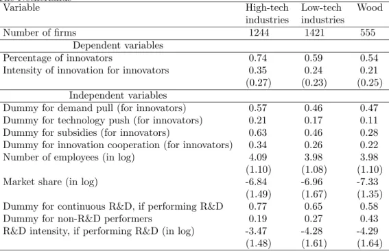
(26) Table 9: Descriptive statistics for the high-tech, low-tech, and wood categories: Means and standard deviation in parentheses for continuous variables: CIS 2.5 The Netherlands Variable High-tech Low-tech industries industries Number of firms 1244 1421 Dependent variables Percentage of innovators 0.74 0.59 Intensity of innovation for innovators 0.35 0.24 (0.27) (0.23) Independent variables Dummy for demand pull (for innovators) 0.57 0.46 Dummy for technology push (for innovators) 0.21 0.17 Dummy for subsidies (for innovators) 0.63 0.46 Dummy for innovation cooperation (for innovators) 0.34 0.26 Number of employees (in log) 4.09 3.98 (1.10) (1.08) Market share (in log) -6.84 -6.96 (1.49) (1.67) Dummy for continuous R&D, if performing R&D 0.77 0.65 Dummy for non-R&D performers 0.19 0.27 R&D intensity, if performing R&D (in log) -3.47 -4.28 (1.48) (1.61). high- and low-tech category of our classification, while it belongs to the low-tech category of the OECD classification. However, our classification could have been more different from the OECD classification had we considered a finer industrial aggregation. There are many more differences between our classification and the Pavitt classification. First of all, our low-tech category comprises both the supplierdominated and the scale intensive categories of the Pavitt classification. More specifically, the industries of food, metallic and non-metallic products of our lowtech category fall into the scale intensive category, while the industries of textile and products not elsewhere classified fall into the supplier-dominated category. Secondly, the industry of wood, which falls into the supplier-dominated category of the Pavitt classification, again behaves differently from the remaining manufacturing industries. Finally, our high-tech category consists essentially of industries that are called science-based in the Pavitt classification with two exceptions regarding the industries of M&E and vehicle that fall respectively into the supplier-dominated and the scale intensive categories of the Pavitt classification.. 5.3. Innovation policy implications. The three categories of firms have different innovative behavior. Hence, innovation policy makers use have different instruments to stimulate innovation according to the category that a firm belongs to. In order to derive possible. 24. Wood 555 0.54 0.21 (0.25) 0.47 0.11 0.28 0.22 3.98 (1.10) -7.33 (1.35) 0.58 0.43 -4.29 (1.64).

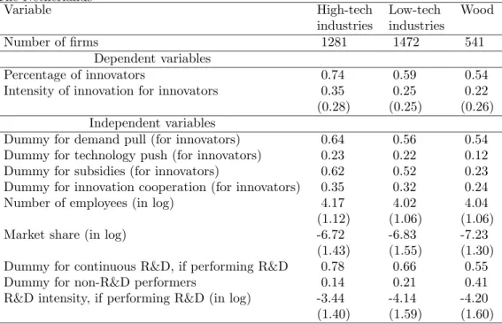
(27) Table 10: Descriptive statistics for the high-tech, low-tech, and wood categories: Means and standard deviation in parentheses for continuous variables: CIS 3 The Netherlands Variable High-tech Low-tech industries industries Number of firms 825 893 Dependent variables Percentage of innovators 0.74 0.61 Intensity of innovation for innovators 0.34 0.25 (0.26) (0.24) Independent variables Dummy for demand pull (for innovators) 0.72 0.70 Dummy for technology push (for innovators) 0.25 0.20 Dummy for subsidies (for innovators) 0.67 0.51 Dummy for innovation cooperation (for innovators) 0.37 0.28 Number of employees (in log) 4.49 4.39 (1.14) (1.02) Market share (in log) -6.39 -6.37 (1.49) (1.57) Dummy for continuous R&D, if performing R&D 0.82 0.68 Dummy for non-R&D performers 0.19 0.28 R&D intensity, if performing R&D (in log) -3.42 -4.31 (1.45) (1.59). innovation policies, we shall discuss the estimated coefficients of the explanatory variables which are to be understood as innovation policy instruments. In the industry of wood, the reference group is an enterprise that performs R&D occasionally, having no innovation cooperation of any kind, for which neither demand pull nor technology push are important, and not being granted innovation subsidies. In the high-tech and low-tech categories, the reference group is an enterprise having the same characteristics as above, and that belongs to the industries of chemicals products and products not elsewhere classified respectively. Findings derived from our study are compared with findings derived from previous empirical studies. Such findings can be found in Table 11. 5.3.1. The selection equation. Size According to the Schumpeterian tradition, the size of an enterprise influences positively the decision by this enterprise to engage in innovation activities, e.g. R&D, as well as the probability to be a product innovator (Brouwer and Kleinknecht (1996)). All empirical studies considered in Table 11 find such an evidence. Size always affects positively and significantly the probability to innovate in our low-tech category. Hence, from an innovation policy standpoint, to encourage non-innovating firms to become innovators, letting firms grow in size is good for innovation. The effect of size is less evident for the high-tech category and the industry of wood. 25. Wood 386 0.52 0.20 (0.23) 0.63 0.14 0.26 0.25 4.27 (1.02) -6.84 (1.28) 0.57 0.43 -4.37 (1.78).

(28) Table 11: Empirical findings from studies on the determinants of innovation in manufacturing using the Community Innovation Survey Study Size Relative Dem. Tech. Coope Performing R&D Contin. Subsidy size pull push ration R&D intensity R&D Probability to innovate 1. Brouwer and + effect n.a + effect n.a no effect n.a + effect + effect n.a Kleinknecht, 1996. 26. 2. Crépon et al. 1998. n.a. n.a. n.a. n.a. n.a. n.a. n.a. n.a. n.a. 3. Mohnen and Dagenais, 2001. + effect. n.a. + effect∗∗. n.a. n.a. n.a. n.a. n.a. n.a. 4. Mairesse and Mohnen, 2001. + effect. n.a. n.a. n.a. n.a. n.a. n.a. n.a. n.a. 5. Janz and Peters, 2002. + effect. no effect. n.a. n.a. n.a. n.a. n.a. n.a. n.a. 6. Janz et al., 2003. + effect. n.a. n.a. n.a. n.a. n.a. n.a. n.a. n.a. 7. Raymond et al., 2004. + effect†. + effect∗†. n.a. n.a. n.a. n.a. n.a. n.a. n.a. 1. Brouwer and Kleinknecht, 1996. - effect. n.a. + effect. + effect. n.a. 2. Crépon et al. 1998. no effect. n.a. + effect. + effect. n.a. n.a. + effect. n.a. n.a. 3. Mohnen and Dagenais, 2001. no effect. n.a. + effect∗∗. n.a. no effect. n.a. no effect. + effect. n.a. 4. Mairesse and Mohnen, 2001. + effect. n.a. + effect. no effect. no effect. + effect†. + effect‡. + effect‡. n.a. 5. Janz and Peters, 2002. + effect. n.a. no effect. no effect. n.a. n.a. n.a. n.a. n.a. 6. Janz et al., 2003. - effect∗. n.a. no effect. no effect. n.a. n.a. n.a. n.a. - effect§. Innovation output: share of innovative sales + effect n.a no effect n.a. †. 7. Raymond et - effect n.a + effect no effect + effect‡§ + effect§§ + effect∗† + effect∗† + effect‡ al., 2004 ∗∗ only for Ireland; † only for low-tech industries; ‡ only for high-tech industries; ∗ only for Germany; § only for Sweden, ∗† only for high- and low-tech industries; ‡§ there is some evidence for the three categories; §§ there is some evidence for high- and low-tech industries;.

(29) Market share The variable ‘relative size’, as measured by the market share of an enterprise, plays a positive role, except for CIS 3, in the probability to innovate for the hightech and low-tech categories. The effect of this variable on the probability to innovate is stronger for the high-tech category than for the low-tech category. This variable never matters for the industry of wood. It should be noticed that, when size is included together with the market share as explanatory variables, the effect of size may turn out not to affect the probability to innovate since both variables are highly correlated. Furthermore, when controlling for technological opportunities and appropriability, the size or market share effect on the probability to innovate may be insignificant (Crépon et al. (1996)). We assume that technological opportunities and appropriability are captured by industry dummies, in the sense that it is easier to innovate in some industries than in others, and that the way of appropriability of innovation differs with different industries. 5.3.2. The regression equation. Size The literature on the determinants of innovation reveals that there is mixed evidence with regard to the effect of size on the share of innovative sales in total sales given that a firm is an innovator. Our finding is in accordance with Brouwer and Kleinknecht (1996), and Janz et al. (2003), i.e., for the three CIS and for each category, smaller innovators are more successful than the larger counterparts. In other words, smaller innovators introduce more new or improved products onto the market than the larger counterparts. Another explanation is that, new or improved products introduced onto the market by smaller firms undergo a more rapid diffusion than new or improved products introduced by larger firms. Hence, from a policy standpoint, in order to stimulate innovation, innovative SMES should be promoted as opposed to monolithic innovators. While size is good for getting firms onto the innovation board wagon, at least in low-tech industries, it rather seems to stand in the way of getting innovators less successful and should therefore not be pursued in this regard. This holds for all industries. Demand pull On the basis of the Schmookler tradition, many empirical studies on the determinants of innovation include the variable ‘demand pull’ as an explanatory variable of innovation. Regardless of the proxy used for ‘demand pull’, a majority of these studies find a positive impact on innovation output intensity. Our finding is in accordance with these studies. In other words, for each category and during the three periods under review, the variable ‘demand pull’ has a positive impact on the share of innovative sales in total sales. Technology push Schumpeter’s tradition reveals that ‘technology push’ enhances innovation. However, many empirical studies find no evidence with regard to the positive 27.