CIRPÉE
Centre interuniversitaire sur le risque, les politiques économiques et l’emploi
Cahier de recherche/Working Paper 06-34
Poverty, Inequality and Stochastic Dominance, Theory and
Practice: Illustration with Burkina Faso Surveys
Abdelkrim Araar
Octobre/October 2006
_______________________
Araar: Département d’économique CIRPÉE and PEP, Pavillon DeSève, Université Laval, Québec, QC Canada G1K 7P4; Fax: 1-418-656-7798
Abstract:
In this paper we provide a set of rules that can be used to check poverty or inequality dominance using discrete data. Existing theoretical rules assumes continuity in incomes or in percentiles of population. In reality, with the form of household surveys, this continuity does not exist. However, the said discontinuity can be exploited in testing the stochastic dominance. Moreover, in this paper, we propose the stochastic dominance conditions that take into account the statistical robustness in testing the stochastic dominance. Findings of this paper are illustrated using the Burkina Faso’s household surveys for the years of 1994 and 1998.
Keywords: Stochastic Dominance, Poverty, Inequality JEL Classification: D 3 6 , D 6 4
1 Introduction
There are several indices used in the literature to measure poverty and inequal-ity. However, some disadvantage can arise by using them especially in comparing between distributions for poverty or inequality. In some instances, the ranking of different distributions may vary depending on the measure of inequality or poverty that is being used1. This is essentially explained by the differences in sensitivity
of these indices at different parts of the distribution or income level. For some distributions, the use of stochastic dominance makes it possible to draw most ro-bust conclusion about ordinal comparaison. It should be noted that the stochastic dominance for a given social order is not based on a pre-determined functional form, but rather on some desirable proprieties or axioms that the corresponding class of indices should respect.
The stochastic dominance approach is useful to establish a robust ordinal com-parison. However, at this point, there exists no theoretical framework with special focus on stochastic dominance with discrete data. This suggests the need to de-velop fundamental rules for the case of discontinuity. Furthermore, most empirical studies lack the statistical tests for the stochastic dominance. For this, we discuss conditions concerning the statistical robustness of the stochastic dominance.
The paper is organized as follows. In section 2, we review briefly the basic theoretical approach to check the stochastic dominance in poverty. In section 3, we develop the general rules to check the stochastic dominance with discrete data. Again, in section 4, we propose some rules to check the stochastic dominance in inequality using Lorenz curves. We discuss in section 5 about the statistical robustness of the stochastic dominance. In section 6, we illustrate findings of this paper by using Burkina Faso surveys for years 1994 and 1998. Conclusions and remarks are reported in section 7.
2 Basic Theoretical Framework
Atkinson (1987) introduced the idea of restricted dominance in poverty. The theoretical poverty dominance conditions have been further and rigorously estab-lished in Foster and Shorrocks (1988 a) and Foster and Shorrocks (1988 b), while bounds to poverty dominance were discussed in Davidson and Duclos (2000). The main aim of using the stochastic dominance approach is to establish a robust or-dinal ranking in poverty, inequality or social welfare based on the adopted social
ethical judgments. The sensitivity of the quantitative indices is not the same at different parts of the distribution. This suggests that ordinal rankings can be re-versed using different indices. We note the class of the additive poverty indices that respect the s ethical order by Ψs(z+), where z+ stands for the upper bound
of the range of possible poverty lines. Additive poverty indices takes the general form:
P (z) =
Z ymax
ymin
υ(y; z)dF (y) (1)
where υ(y; z) is the poverty indicator or contribution of household with income y to the poverty index. Suppose that the additive poverty indices respect the focus axiom, then: υ(y; z) = 0 if y ≥ z. For the first class of poverty indices noted by Ψ1(z+), these indices will be unchanged or will decrease with an increase in
income or standard living of the poor household. Ψ1(z+) = ½ P (z) ¯ ¯ ¯ ¯ υ (1) y (y; z) ≤ 0 when y ≤ z z ≤ z+, ¾ (2) where υy(1)(y; z) is the first derivative of υ in y. The second class of poverty indices
Ψ2(z+):
• belong to the first-order class
• are convex in living standards or income y. Also, this implies that these
in-dices respect the Pigou-Dalton principle, such that a marginal income trans-fer from a richer-poor to a poorer-poor reduces poverty.
Ψ2(z+) = P (z) ¯ ¯ ¯ ¯ ¯ ¯ P (z) ∈ Ψ1(z+), υ(2)y (y; z) ≥ 0 when y ≤ z, υ(z; z) = 0. (3)
The third class of poverty indices concerns indices that:
• belong in the second class.
• are decreasing in the following composite transfer:
– a beneficial Pigou-Dalton transfer within the lower part of the distri-bution accompanied by an adverse Pigou-Dalton transfer within the upper part of the distribution
Ψ3(z+) = P (z) ¯ ¯ ¯ ¯ ¯ ¯ P (z) ∈ Ψ2(z+), υ(3)(y; z) ≤ 0 when y ≤ z, υ(z, z) = 0 and υ(1)(z, z) = 0. (4)
In general, poverty indices will be members of class Ψs(z+) if (−1)sυ(s)
y (y; z) ≤
0 and if υ(i)(z, z) = 0 for i = 0, 1, 2..., s − 2. As the order s of the class of poverty
indices increase, these indices become more and more sensitive to the distribution of income among the poorest. As proposed by Davidson and Duclos (2000), to check the stochastic dominance for the order s, one can compare between domi-nance curves that take the following form:
Ds(z) = 1 (s − 1)! Z ymax ymin (z − y)s +dF (y) (5)
where (z − y)+ = (z − y) if z > y and zero otherwise. One can remark that this
curve is simply a monotonic transformation of the FGT curve. Based on this, one can use the FGT curves directly to check the poverty dominance. The dominance curve can be expressed as follows:
Ds(z) = cP (α = s − 1, z) (6)
where c = 1/(s − 1)! is a constant term. The distribution B dominates in poverty the distribution A for the order s = α + 1 if:
∆α(z) = PA(α, z) − PB(α, z) > 0 ∀z ∈ [0, ∞] (7)
where P (α, z) is the FGT index. Dominance here refers to the distribution that generates more social welfare or less poverty. Usually, one checks the dominance between two distributions for the followings:
• two successive periods for the same country. • two groups in the same country.
• two countries.
3 Poverty and Dominance Testing
3.1 The numerical approach
One of the simplest numerical approach is the Grid Approach. The procedure is based on the comparison between two curves for a range of poverty lines z
or percentiles p with fixed step. If the two curves crossed, then a simple linear approximation is used to estimate the critical value. However, this approach have the following drawbacks:
• If there are two successive intersections within the step, the intersections
cannot detected.
• Using a short step is costly in computations and requires more time. • The linear approximation continues to have some residual error.
3.2 The theoretical approach
With discrete data, we propose to develop the main rules that can be used to consistently check the dominance for the three widely used orders, the first, second and the third. If we note the income for household i, that belongs to distribution D, by yD
i and its proportion in the population by πiD the distribution
D is defined as follows:
D(Y, Π) =©yD
i , πDi |i ∈ D
ª
(8) Suppose that the two distributions A and B are combined and are sorted by the vector of income Y , to form one data set which takes the following form:
S = {A, B} = {yi, πiA|S, π B|S
i |i ∈ S} (9)
where πD|Si = πD
i if i ∈ D and zero otherwise. The final step for the treatment of
the data is to aggregate them by summing proportions πiD|S according to Y . This procedure ensures that there is only a unique value for each yi ∈ S. In annex A,
we give an illustrative example to explain these steps in clear way. Lemma 1
PD(α, z) = PSD(α, z) (10)
where PD
S (α, z) is the FGT index when the distribution {yi, πA|Si } is used. This
lemma indicates that poverty indices do not change with the rearrangement of the data.
Lemma 2
∆α(z) > 0 ∀z ∈£ySmin, ymaxS ¤⇔ ∆α(z) > 0 ∀z ∈ [yi, yi+1[
where NS is the size of the combined distributions S, yminS and ySmax are the
minimum and maximum level of incomes respectively. This lemma indicates that checking the stochastic dominance condition within the range £yS
min, ySmax
¤ is equivalent to checking this dominance between ranges, formed by the discrete data.
Theorem 3 Between two successive points yiand yi+1∈ Y .
A: If ∆α=0(y
i) > 0 , then ∆α=0(z) > 0 ∀z ∈ [yi, yi+1[.
B: If ∆α=0(y
i) 6= 0 and ∆α=0(yi) ∗ ∆α=0(yi+1) < 0, then the unique
intersec-tion is equal to yi+1.
C: If ∆α=0(y
i) = 0, then the range of intersections will be [yi, yi+1[.
Proof.
A: The curve ∆α=0(z) takes a horizontal form for the range z ∈ [y
i, yi+1[.
B: The sign of ∆α=0(z) changes after introducing the observation y
i+1and the
difference increases or decreases vertically at yi+1.
C: See [A:].
Theorem 4 Between two successive points yi and yi+1 ∈ Y , the maximum
num-ber of intersections, between the two curves of dominance for the order s ≥ 2, is
(s − 1).
Proof. Since between yi and yi+1 there are no any additional changes except the
increase of the poverty line z, the difference between the two curves takes the following polynomial form:
∆α=(s−1)(z) = s
X
s=1
aszs−1 (12)
where as are known parameters. Polynomial with degree s, has exactly s roots,
real or complex.
Corollary 5 There is only one intersection between two successive points, yiand
yi+1if:
∆α=1(y
Proof. Based on theorem 4, the function ∆α=1(z) takes a linear form between
yi, yi+1such that ∆α=1(z) = a1+ a2z. Solving the equation: a1+ a2z = 0 gives
us a unique root.
Theorem 6 Consider two successive points yiand yi+1∈ Y . We have:
∆α=1(y
i) > 0 and ∆α=1(yi+1) > 0 ⇒ ∆α=1(z) > 0 ∀z ∈ [yi, yi+1] (14)
Proof. Based on theorem 4, the function ∆α=1(z) takes a linear form between
yi, yi+1such that ∆α=1(z) = a1+ a2z. Since ∆α=1(yi) > 0 and ∆α=1(yi+1) > 0,
the level of the curve ∆α=1(z) should be higher than zero for all z ∈ [y
i, yi+1].
Theorem 7 Consider two successive points yiand yi+1∈ Y , such that:
∆α=2(y
i) > 0 and ∆α=2(yi+1) > 0 (15)
A: If ∆α=1(y
i) ≥ 0 and ∆α=1(yi+1) ≥ 0, then ∆α=2(z) > 0 ∀z ∈ [yi, yi+1]
B: If ∆α=1(y
i) < 0 and ∆α=1(yi+1) > 0, then the maximum number of
inter-sections is two.
Proof.
A: The level of ∆α=2(z) for z ∈ [y
i, yi+1], depends on the initial value ∆α=2(yi)
and the tangency of ∆α=2(z) within this interval. If the tangency ∆α=1(z) ≥
0 ∀z ∈ [yi, yi+1], the increase of z does not decrease the initial difference.
Since it is supposed that the condition: ∆α=1(y
i) > 0 and ∆α=1(yi+1) > 0
is satisfied and based on the theorem 6, the tangency ∆α=1(z) ≥ 0 ∀z ∈
[yi, yi+1].
B: See theorem 4 for the possible number of intersections.
Theorem 8 Let two successive points yiand yi+1∈ Y . If the following conditions
are satisfied:
∆α=2(yi) > 0 and ∆α=2(yi+1) < 0 (16)
∆α=1(y
i) < 0 and ∆α=1(yi+1) < 0 (17)
Proof. Since the tangency ∆α=1(z) ≤ 0 ∀z ∈ [y
i, yi+1], the difference between
the two curves continues to decrease between yi, yi+1and its value is null only for
one critical value of z.
This theoretical framework is very useful to design founded procedures to test the stochastic dominance or to estimate all possible critical values accurately. Condition of continuous checking within the interval [yi, yi+1] is simplified with
discrete distributions to bounds of this interval.
3.3 Estimating the critical values
In this context, by critical values we refer to the level of poverty line for which two dominance curves cross. We restrict the discussion here to the three widely used dominance orders; the first, the second and the third order. Within the interval [yi, yi+1], the three main cases that one would encounter are: For case C, the
Case Difference A ∆α(y i) > 0 and ∆α(yi+1) < 0 B ∆α(y i) < 0 and ∆α(yi+1) > 0 C ∆α(y i) = 0
estimation of the critical value, noted by z∗, is trivial and equals y i.
3.3.1 Critical values for the first order dominance
For the first order s = 1, for the two cases A and B, the critical value equals to yi+1. The sign of the difference in headcount ∆α=0(z = yi) =
Pi
j=1πjA−
Pi
j=1πjB changes after introducing the observation yi+1 and the curve ∆α=0(z)
increases or decreases vertically.
3.3.2 Critical values for the second order dominance
For the two main cases A and B, we have to solve this simple following equa-tion: i X j=1 πA j z − i X j=1 πA j yj = i X j=1 πB j z − i X j=1 πB j yj (18)
The critical value equals to: z∗ = HiA∗ µAi − HiB∗ µBi HB i − HiA (19) where HD
i and µDi are respectively the headcount and the average income of the
poor group when z = yi.
3.3.3 Critical values for the third order dominance
We discuss the possible intersections for case A (the discussion of case B is similar). Based on theorems 7 and 8, and where the intersections are possible we have that:
∆α=2(z∗) = 0 and z∗ ∈ [y
i, yi+1] (20)
To estimate the valid intersections, one should solve the following equation:
i X j=1 πA j ¡ z2− 2zy j + y2j ¢ − i X j=1 πB j ¡ z2− 2zy j+ yj2 ¢ = 0 (21) One can rewrite this equation as follows:
a3z2+ a2z + a1 = 0 and z ∈ [yi, yi+1] (22)
where, ai are known parameters, such that:
a1 = (HiA∗ ωAi − HiB∗ ωiB)
a2 = 2(HiB∗ µBi − HiA∗ µAi )
a3 = HiA− HiB
(23) where ωD
i is the average of square incomes for the group with income below or
equal to yi.
4 Inequality and Stochastic Dominance Test
The widely used approach to test the stochastic dominance in inequality is the comparison between the Lorenz curves. According to Atkinsons Theorem 2, all
indices that respect the Pigou-Dalton principe should indicate that inequality in A
is higher than inequality in B when LB(p) be everywhere above LA(p). Formally,
distribution B dominates distribution A in inequality, with the second order, if3:
LA(p) > LB(p) ∀p ∈ [0, 1] (24)
where p refers to the percentile. Again here, one can propose some general rules to check for the stochastic dominance in the presence of discrete data sets. Recall that the Lorenz curve for the percentile pi can be defined as follows:
L(p = pi) = 1 µ i X j=1 πjyj (25)
The main characteristics of the Lorenz curve with discrete data, is the straight line that ties L(pi) and L(pi+1). This implies that the difference between two
Lorenz curves takes a straight line format between two successive percentiles de-rived from these two distributions. Hence, the first step is to combine the two percentile vectors of the two distributions. Then we estimate the Lorenz curves for all retained values of this new vector of percentiles (see again the illustrative example in Annex B). We define the difference between two Lorenz curves for the percentile p by ∆(p).
Theorem 9 Let two successive percentiles pi, pi+1.
If: ∆(pi) > 0 and ∆(pi+1) > 0 , then ∆(p) > 0 ∀p ∈ [pi, pi+1]
Theorem 10 Between two successive percentiles pi, pi+1, the maximum number
of intersection between the Lorenz curves is one.
Theorem 11 There is only one intersection between two successive percentiles
pi, pi+1if: ∆(pi) ∗ ∆(pi+1) < 0.
One can generalize this and confirm that these rules are always valid for the com-parison between the generalized Lorenz curves, the Lorenz and the concentration curves or between the TIP (Three I’s Poverty) curves4.
3The distribution dominates in inequality when its level in inequality is the lower. The decrease
in inequality generates more social welfare.
4TIP curves shows simultaneously the Incidence, Intensity of poverty and Inequality within
5 Statistical Robustness of the Stochastic Dominance
5.1 Stochastic dominance with statistical robustness
Despite the fact that one can estimate the difference between the two distribu-tional curves to check the stochastic dominance for welfare, poverty or inequality, this difference may not be statistically significant. Our interest here is to check if the stochastic dominance is statistically robust. One can again estimate the critical values according to the selected statistical significance level.
Proposition 12 The dominance in poverty for the order s is statistically robust if
the difference between the two dominance curves is statistically significant for all poverty line z ∈ [0, ∞].
For the (α + 1)th order of dominance, the statistical robustness of the stochastic
dominance is satisfied with a critical level of significance θ, if the following null hypothesis H0 is rejected ∀z ∈ [0, ∞].
H0 : ∆α(z) ≤ 0 against H1 : ∆α(z) > 0 (26)
The null hypothesis is rejected if: d
LB∆α(z) = ˆ∆α(z) − ˆδ∆(z)Cθ > 0 (27)
where LB∆α(z) is the lower bound of the confidence interval, ˆδ∆(z) is the
esti-mated standard deviation and Cθ refers to the cumulative distribution of the
esti-mated parameter ˆ∆α(z), evaluated at the critical significance level θ. Generally,
the distribution of the estimate takes the t-student form with the smallest number of observations. When the number of observations or the degree of freedom is higher, this distribution converges to the normal form. Estimation of the standard errors ˆδ∆(z) depends again on the sampling design of the two distributions5.
Proposition 13 For the second order dominance in inequality and based on the
comparison between Lorenz curves, dominance in inequality is statistically robust if the difference between the two Lorenz curves is statistically significant ∀p ∈
[0, 1].
5.2 Critical values with statistical robustness
Critical values with the statistical robustness refers to the limits of the poverty line z or the percentile p where the statistical robustness of the dominance tinues to be checked. Note that the critical values, with statistical robustness con-dition, can be different from those based only on basic theoretical conditions of dominance.
6 Illustration Using Burkina Faso National Surveys
The two nationally representative Burkina Faso’s surveys used in this study, were carried out in 1994 and 1998. These surveys were made with sample se-lection using two-stage stratified random sampling method. The country was stratified into seven in 1994 and ten in 1998. For the survey of 1994, five of these strata were rural and two were urban. Enumeration areas ( PSU’s, or zones
de d´enombrement) were sampled in the first stage from a census list prepared
in 1985. In the first-stage, sampling was done in stratum 7 (Ougadougou-Bobo-Dioulasso) with equal probability and for the other 6 strata sampling was done with probability proportional to the size of each PSU. Twenty households were then systematically sampled within each of the selected PSU’s in a second stage. The survey of 1998 is similar to that of 1994.
The consumption per capita is used to represent the household living standard. For the year 1998, consumption is deflated by the ratio of poverty lines of the two periods. We use the Stata modules, that I have developed based on theoretical findings of this paper, to perform the estimations6.
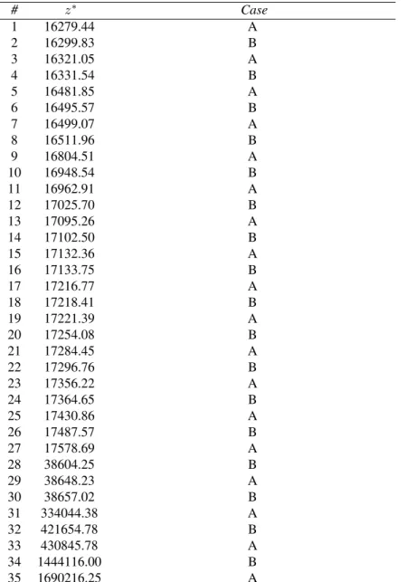
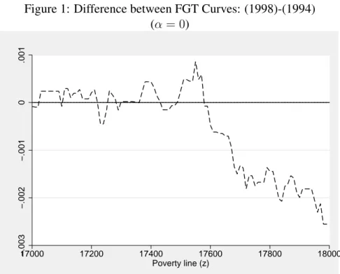
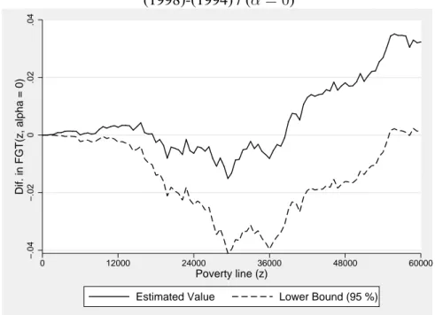
Figures 1 and 2 show the difference between the FGT curves where the pa-rameter α equals to zero. Note that the dominance condition is not satisfied and that the two dominance curves cross, as reported in table 1. One can recall here that the official poverty line in Burkina Faso was 41099 F CFA for the referenced year of 1994. Even if one restricts the range of all possible poverty lines around this official line, intersections are encountered when the poverty line is between 35 000 and 45 000 F CFA.
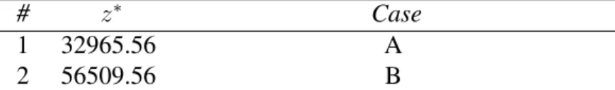
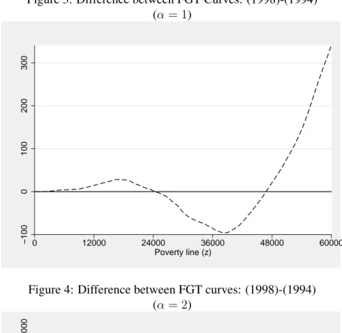
Figures 3 shows that the condition of dominance is not satisfied for the second order. Intersections between dominance curves are presented in tables 2. For a re-stricted range of poverty line between 35 000 and 45 000 F CFA, intersections are
6The Stata modules povdom.ado and ineqdom.ado perform the test of dominance and estimate
not encountered and the deficit of poverty was decreased in 1998. For the severity indices of poverty, one cannot draw a robust conclusion, since intersections are encountered as presented in figure 4 and table 3. Figures 5 and 6 show again the difference between the FGT curves and the lower bound of the estimated differ-ence 7. One can see that with or without the statistical robustness, conditions of
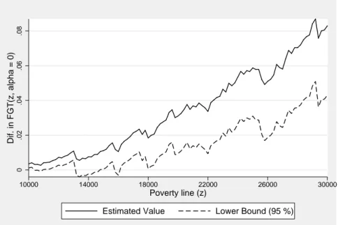
dominance are generally not satisfied. In figure 7 we show that, without statistical robustness condition, female headed households dominate in poverty male headed households for the year 1994. By adding the statistical robustness condition, the stochastic dominance is not checked.
With respect to the dominance in inequality for these two periods, figure 8 and table 4 show that the Lorenz curves cross for two percentiles. Again here, one cannot draw a robust conclusion about the variation in inequality between these two periods.
7 Conclusion
Comparing levels of poverty or inequality between distributions remains a ma-jor issue of interest to both researchers and policy makers. In the last quarter of the century, several countries have experienced important changes in their economies which triggered changes in distribution channels of income or wealth. In gen-eral, quantitative indices were mostly used to assess the evolution of poverty or inequality. This approach can be criticized, where quantitative indices differ in their sensitivities for the different parts of the distribution. Stochastic dominance approach allows us in some cases to make a robust ordinal classification of dis-tribution according to their level in poverty or in inequality. Existing theoretical frameworks were built under the assumption of continuity of incomes. This paper treats the case of discontinuity or discrete distributions. This is justified by the fact that household surveys have a discrete form. Also, in this paper we propose some conditions for testing the statistical robustness of the stochastic dominance. More importantly, these statistical conditions can change our conclusions about the dominance. Methods and findings of this paper are illustrated with the Burk-ina Faso household surveys for the years 1994 and 1998. In general, results of this application show that one cannot draw a robust conclusion on changes of poverty or inequality between these two periods. This is explained substantially by the
7We have taken into account the sampling design in carrying out the estimation of standard
errors and bounds of confident interval. Stata modules, that I have developed for these estimations are cdifgt.ado and cdilorenz.ado. These modules can be provided upon request.
non significance level of change in the distribution of standard of livings between these two periods.
Table 1: Intersection between FGT curves (α = 0) # z∗ Case 1 16279.44 A 2 16299.83 B 3 16321.05 A 4 16331.54 B 5 16481.85 A 6 16495.57 B 7 16499.07 A 8 16511.96 B 9 16804.51 A 10 16948.54 B 11 16962.91 A 12 17025.70 B 13 17095.26 A 14 17102.50 B 15 17132.36 A 16 17133.75 B 17 17216.77 A 18 17218.41 B 19 17221.39 A 20 17254.08 B 21 17284.45 A 22 17296.76 B 23 17356.22 A 24 17364.65 B 25 17430.86 A 26 17487.57 B 27 17578.69 A 28 38604.25 B 29 38648.23 A 30 38657.02 B 31 334044.38 A 32 421654.78 B 33 430845.78 A 34 1444116.00 B 35 1690216.25 A
Case A: Distribution 1 dominates distribution 2 before the intersection Case B: Distribution 2 dominates distribution 1 before the intersection
Table 2: Intersection between FGT curves (α = 1)
# z∗ Case
1 24262.87 A
2 46775.65 B
Case A: Distribution 1 dominates distribution 2 before the intersection Case B: Distribution 2 dominates distribution 1 before the intersection
Table 3: Intersection between FGT curves (α = 2)
# z∗ Case
1 32965.56 A
2 56509.56 B
Case A: Distribution 1 dominates distribution 2 before the intersection Case B: Distribution 2 dominates distribution 1 before the intersection
Table 4: Intersection between Lorenz curves: (1994) vs. (1998)
# p∗ Case
1 0.048857 B
2 0.791681 A
Case A: Curve 1 is bellow Curve 2 before the intersection Case B: Curve 1 is above Curve 2 before the intersection
Figure 1: Difference between FGT Curves: (1998)-(1994) (α = 0) −.003 −.002 −.001 0 .001 17000 17200 17400 17600 17800 18000 Poverty line (z)
Figure 2: Difference between FGT Curves: (1998)-(1994) (α = 0) −.002 0 .002 .004 .006 38500 38600 38700 38800 38900 39000 Poverty line (z)
Figure 3: Difference between FGT Curves: (1998)-(1994) (α = 1) −100 0 100 200 300 0 12000 24000 36000 48000 60000 Poverty line (z)
Figure 4: Difference between FGT curves: (1998)-(1994) (α = 2) −2000000 −1000000 0 1000000 2000000 0 12000 24000 36000 48000 60000 Poverty line (z)
Figure 5: Difference between FGT Curves and the statistical robustness (1998)-(1994) / (α = 0) −.04 −.02 0 .02 .04 Dif. in FGT(z, alpha = 0) 0 12000 24000 36000 48000 60000 Poverty line (z)
Estimated Value Lower Bound (95 %)
Figure 6: Difference between FGT curves and the statistical robustness (1998)-(1994) / (α = 1) −1000 −500 0 500 Dif. in FGT(z, alpha = 1) 0 12000 24000 36000 48000 60000 Poverty line (z)
Figure 7: Difference between FGT curves according to the gender of household head: (Male)-(Female): Burkina Faso 1994 (α=0)
0 .02 .04 .06 .08 Dif. in FGT(z, alpha = 0) 10000 14000 18000 22000 26000 30000 Poverty line (z)
Estimated Value Lower Bound (95 %)
Figure 8: Difference between Lorenz curves (1998)-(1994) −.04 −.02 0 .02 .04 Dif. in L(p) 0 .2 .4 .6 .8 1 Percentiles (p)
References
ARAAR, A. (2006): DASP: Distributive Analysis Stata Package., Laval Uni-versity, PEP & CIRPEE.
ARAAR, A. AND J.-Y. DUCLOS (2005): “An Atkinson-Gini Family of So-cial Evaluation Functions: Theory and Illustration using Data from the Luxembourg Income Study,” Tech. Rep. LIS-WP: 416.
ATKINSON, A. B. (1970): “On the Measurement of Inequality,” Journal of Economic Theory, 2, 244–63.
——— (1987): “On the Measurement of Poverty,” Econometrica, 55, 749 –764.
DAVIDSON, R. AND J.-Y. DUCLOS (2000): “Statistical Inference for Stochastic Dominance and the for the Measurement of Poverty and In-equality,” Econometrica, 68, 1435–1465.
DUCLOS, J. Y. AND A. ARAAR (2006): Poverty and Equity Measure-ment, Policy, and Estimation with DAD, Boston/Dordrecht/London:
Springer/Kluwer Academic Publishers.
FOSTER, J. E. AND A. F. SHORROCKS (1988 a): “Poverty Orderings,” Econometrica, 56, 173–177.
——— (1988 b): “Poverty Orderings and Welfare Dominance,” Social
Choice Welfare, 5, 179–98.
JENKINS, S. P. AND P. J. LAMBERT(1998): “,Three ’I’s of Poverty Curves and Poverty Dominance: TIPs for Poverty Analysis,” Research on
ANNEX A: Illustrative example 1
Data A Data B Combined Data: S YA ΠA YB ΠB Y ΠA|S ΠB|S
13 0.4 13 0.3 13 0.4 0.6 15 0.6 13 0.3 15 0.6 0
30 0.4 30 0 0.4
ANNEX B: Illustrative example 2
Data A Data B Combined Data: S
YA pA LA(p) YB pB LB(p) p LA(p) LB(p) – 0.0 .0000 – 0.0 .0000 0.0 .0000 .0000 3 0.1 .0441 2 0.1 .0408 0.1 .0441 .0408 5 0.4 .2647 3 0.4 .2245 0.4 .2647 .2245 7 0.6 .4706 4 0.5 .3061 0.5 .3676 .3061 9 1.0 1.0000 6 0.8 .6735 0.6 .4706 .4286 8 1.0 1.0000 0.8 .7353 .6735 1.0 1.0000 1.0000