HAL Id: hal-02316446
https://hal.archives-ouvertes.fr/hal-02316446
Submitted on 8 Jan 2021
HAL is a multi-disciplinary open access
archive for the deposit and dissemination of
sci-entific research documents, whether they are
pub-lished or not. The documents may come from
teaching and research institutions in France or
abroad, or from public or private research centers.
L’archive ouverte pluridisciplinaire HAL, est
destinée au dépôt et à la diffusion de documents
scientifiques de niveau recherche, publiés ou non,
émanant des établissements d’enseignement et de
recherche français ou étrangers, des laboratoires
publics ou privés.
Antonietta Capotondi, Michael Jacox, Chris Bowler, Maria Kavanaugh,
Patrick Lehodey, Daniel Barrie, Stephanie Brodie, Samuel Chaffron, Wei
Cheng, Daniela Dias, et al.
To cite this version:
Antonietta Capotondi, Michael Jacox, Chris Bowler, Maria Kavanaugh, Patrick Lehodey, et al..
Ob-servational Needs Supporting Marine Ecosystems Modeling and Forecasting: From the Global Ocean
to Regional and Coastal Systems. Frontiers in Marine Science, Frontiers Media, 2019, 6, pp.623.
�10.3389/fmars.2019.00623�. �hal-02316446�
doi: 10.3389/fmars.2019.00623
Edited by: Tong Lee, NASA Jet Propulsion Laboratory (JPL), United States Reviewed by: Susan Kay, Met Office, United Kingdom Ana Carolina De Azevedo Mazzuco, Federal University of Espirito Santo,
Brazil Stefano Ciavatta, Plymouth Marine Laboratory, United Kingdom *Correspondence: Antonietta Capotondi antonietta.capotondi@noaa.gov
Specialty section: This article was submitted to Ocean Observation, a section of the journal Frontiers in Marine Science Received: 14 November 2018 Accepted: 20 September 2019 Published: 15 October 2019 Citation: Capotondi A, Jacox M, Bowler C, Kavanaugh M, Lehodey P, Barrie D, Brodie S, Chaffron S, Cheng W, Dias DF, Eveillard D, Guidi L, Iudicone D, Lovenduski NS, Nye JA, Ortiz I, Pirhalla D, Pozo Buil M, Saba V, Sheridan S, Siedlecki S, Subramanian A, de Vargas C, Di Lorenzo E, Doney SC, Hermann AJ, Joyce T, Merrifield M, Miller AJ, Not F and Pesant S (2019) Observational Needs Supporting Marine Ecosystems Modeling and Forecasting: From the Global Ocean to Regional and Coastal Systems. Front. Mar. Sci. 6:623. doi: 10.3389/fmars.2019.00623
Observational Needs Supporting
Marine Ecosystems Modeling and
Forecasting: From the Global Ocean
to Regional and Coastal Systems
Antonietta Capotondi1,2* , Michael Jacox2,3,4, Chris Bowler5,6, Maria Kavanaugh7,
Patrick Lehodey8, Daniel Barrie9, Stephanie Brodie3,4, Samuel Chaffron6,10,
Wei Cheng11,12, Daniela F. Dias13, Damien Eveillard6,10, Lionel Guidi6,14,
Daniele Iudicone15, Nicole S. Lovenduski16, Janet A. Nye17, Ivonne Ortiz11,
Douglas Pirhalla18, Mercedes Pozo Buil3,4, Vincent Saba19, Scott Sheridan20,
Samantha Siedlecki21, Aneesh Subramanian22, Colomban de Vargas6,23,
Emanuele Di Lorenzo24, Scott C. Doney25, Albert J. Hermann11,12, Terrence Joyce26,
Mark Merrifield13, Arthur J. Miller13, Fabrice Not6,27and Stephane Pesant28
1Cooperative Institute for Research in Environmental Science, University of Colorado Boulder, Boulder, CO, United States, 2Physical Sciences Division, NOAA/ESRL, Boulder, CO, United States,3Institute of Marine Science, University of California,
Santa Cruz, Santa Cruz, CA, United States,4Environmental Research Division, NOAA Southwest Fisheries Science Center,
Monterey, CA, United States,5Institut de Biologie de l’Ecole Normale Supérieure, Ecole Normale Supérieure, CNRS,
INSERM, Université PSL, Paris, France,6Research Federation for the Study of Global Ocean Systems Ecology
and Evolution, FR2022/Tara Oceans GOSEE, Paris, France,7College of Earth, Ocean, and Atmospheric Sciences, Oregon
State University, Corvallis, OR, United States,8Collecte Localisation Satellites, Ramonville-Saint-Agne, France,9NOAA
Climate Program Office, Modeling, Analysis, Predictions, and Projections, Silver Springs, MD, United States,10LS2N, CNRS
UMR 6004, Université de Nantes, Nantes, France,11JISAO, University of Washington, Seattle, WA, United States,12NOAA
Pacific Marine Environmental Laboratory, Seattle, WA, United States,13Scripps Institution of Oceanography, University
of California, San Diego, La Jolla, CA, United States,14CNRS, Laboratoire d’Océanographie de Villefranche, Sorbonne
Université, Villefranche-sur-Mer, France,15Stazione Zoologica Anton Dohrn, Naples, Italy,16Department of Atmospheric and
Oceanic Sciences and Institute of Arctic and Alpine Research, University of Colorado Boulder, Boulder, CO, United States,
17School of Marine and Atmospheric Sciences, Stony Brook University, Stony Brook, NY, United States, 18NOAA/NOS/NCCOS, Silver Spring, MD, United States,19National Marine Fisheries Service, National Oceanic
and Atmospheric Administration, Northeast Fisheries Science Center, Geophysical Fluid Dynamics Laboratory, Princeton University, Princeton, NJ, United States,20Department of Geography, Kent State University, Kent, OH, United States, 21Department of Marine Sciences, University of Connecticut, Groton, CT, United States,22Department of Atmospheric and
Oceanic Sciences, University of Colorado Boulder, Boulder, CO, United States,23CNRS, Station Biologique de Roscoff,
AD2M ECOMAP, Sorbonne Université, Roscoff, France,24Georgia Institute of Technology, Atlanta, GA, United States, 25Department of Environmental Sciences, University of Virginia, Charlotteville, VA, United States,26Woods Hole
Oceanographic Institution, Woods Hole, MA, United States,27CNRS – UMR 7144 – Ecology of Marine Plankton Group –
Station Biologique de Roscoff, Sorbonne Université, Roscoff, France,28MARUM, Center for Marine Environmental Sciences,
University of Bremen, Bremen, Germany
Many coastal areas host rich marine ecosystems and are also centers of economic activities, including fishing, shipping and recreation. Due to the socioeconomic and ecological importance of these areas, predicting relevant indicators of the ecosystem state on sub-seasonal to interannual timescales is gaining increasing attention. Depending on the application, forecasts may be sought for variables and indicators spanning physics (e.g., sea level, temperature, currents), chemistry (e.g., nutrients, oxygen, pH), and biology (from viruses to top predators). Many components of the marine ecosystem are known to be influenced by leading modes of climate variability, which provide a physical basis for predictability. However, prediction capabilities remain limited by the lack of a clear understanding of the physical and biological processes
involved, as well as by insufficient observations for forecast initialization and verification. The situation is further complicated by the influence of climate change on ocean conditions along coastal areas, including sea level rise, increased stratification, and shoaling of oxygen minimum zones. Observations are thus vital to all aspects of marine forecasting: statistical and/or dynamical model development, forecast initialization, and forecast validation, each of which has different observational requirements, which may be also specific to the study region. Here, we use examples from United States (U.S.) coastal applications to identify and describe the key requirements for an observational network that is needed to facilitate improved process understanding, as well as for sustaining operational ecosystem forecasting. We also describe new holistic observational approaches, e.g., approaches based on acoustics, inspired by Tara Oceans or by landscape ecology, which have the potential to support and expand ecosystem modeling and forecasting activities by bridging global and local observations.
Keywords: marine ecosystems, modeling and forecasting, seascapes, genetics, acoustics
INTRODUCTION
Marine ecosystems, comprising life from microscopic plankton to top predators provide resources and services that are key to the health and well-being of human society. Marine ecosystems also support lucrative industries, such as fisheries, aquaculture, tourism, recreation, and shipping, thus substantially contributing to the Blue Economy. Based on data for 2015, the Blue Economy in the United States (U.S.) accounts for 2.3% of U.S. employment and 1.8% of gross domestic product (GDP) contributing 3.2 million employees and 320 billion dollars in GDP, outpacing the annual growth of the total U.S. economy in both of these areas (National Oceanic and Atmospheric Administration
[NOAA], 2018). Globally, the output of the global ocean
economy is estimated at EUR 1.3 trillion today and this could more than double by 2030 (https://ec.europa.eu/maritimeaffairs/ sites/maritimeaffairs/files/swd-2017-128_en.pdf . The importance of fish for the world economy and food security cannot be overstated, with over 56 million people engaged in fishing and aquaculture, which provide about 7% of the global population’s protein consumption (FAO, 2016).
Coastal and shelf areas play a very special role in the generation of marine resources in that they connect large-scale climate variations with coastal communities. Indeed, almost half of the global economic value of marine fisheries and related industries is associated with fish catches near coastal areas (Nellemann et al., 2008). This complicated management environment resides within a highly variable coastal ocean that responds to local, regionally specific processes, in addition to being subject to global change (Bowen and Riley, 2003;Cloern et al., 2016;Tommasi et al., 2017). Eastern ocean boundaries, in particular, host rich and productive marine ecosystems (Chavez and Messié, 2009) that are supported by coastal upwelling, a wind-driven circulation that brings nutrient-rich deep waters to the near-surface sun-lit layer of the ocean, stimulating growth of phytoplankton that forms the base of the marine food web (Dugdale and Goering, 1967). Besides upwelling, frontal currents, eddies, cross-shelf transport, tides and coastally trapped wave
propagation are also very important physical drivers of marine ecosystems in coastal areas, as they determine upper-ocean temperature and salinity profiles, and directly affect ecosystem characteristics and distribution, e.g., “warm” or “cold” ecosystem states (Checkley and Barth, 2009).
Due to the small spatial scale of key regionally specific coastal processes (e.g., upwelling and topographically stirred along-shore transport), understanding ecosystem dynamics in coastal regions requires observations and ocean models with a sufficiently high spatial and temporal resolution to resolve those scales (Fiechter et al., 2014;Rudnick, 2016;Turi et al., 2018). For example, upwelled water is typically high not only in nutrients but also in inorganic carbon; therefore, recently upwelled waters both outgas CO2to the atmosphere and subsequently stimulate
primary production that draws down CO2. At the same time,
biogeochemical tracers and plankton are transported laterally by Ekman transport as well as eddies, jets, and meanders, which decouples various processes in space. Ultimately these dynamics produce sharp spatial gradients in, for example, carbon fluxes (Fiechter et al., 2014) and plankton and fish community compositions (Rykaczewski and Checkley, 2008), which also vary in response to large-scale climate variability (e.g.,Chavez et al., 2003). Ocean models are key tools for elucidating this type of interplay between processes controlling marine ecosystems. They can be used to simulate complex physical and biological ecosystem dynamics (Rose et al., 2015) and quantify the impacts of different climate drivers (Jacox et al., 2015a). They can also be used to produce accurate estimates of the state of the system by assimilating available observations (Moore et al., 2019), thus facilitating extension of these observational records in space and time beyond what can be obtained from observations alone. In both applications, observations are crucial for initializing, validating, constraining, and improving model behavior.
The functioning of marine ecosystems across all trophic levels is intimately linked to climate variations. Indeed, many economically vital organisms have shown sensitivity to environmental conditions, including low Dissolved Oxygen (DO, e.g.,Froehlich et al., 2014), ocean pH (e.g.,Bednarsek et al., 2017),
sea ice extent (Saba et al., 2014), bottom temperature (Mueter and Litzow, 2008), and marine heatwaves (Oliver et al., 2018). Since these organisms respond strongly to biogeochemical and physical forcing, the right kind of prognostic information could yield significant payoffs for management and industry, and thus make ecosystem services and the Blue Economy more resilient to expected change. In addition, understanding the environmental sensitivity of detrimental biological organisms, such as harmful algal blooms, would also positively impact the Blue Economy. Examples of how both species-specific and community responses can be combined with beta-diversity relationships to disentangle complex ocean-climatic processes have emerged from extensive analysis of Tara Oceans data, specifically to provide new insights into carbon export and iron bioavailability (Guidi et al., 2016; Caputi et al., 2019, see section Toward Holistic Marine Ecosystems Monitoring for Improving Ocean Models).
The connection between climate and marine ecosystem encompasses a broad range of timescales. Seasonal variations of insolation, wind intensity and direction, and river runoff directly affect primary production by modulating light and nutrient availability for photosynthesis. At interannual timescales, the El Niño Southern Oscillation (ENSO) in the tropical Pacific has profound impacts on marine ecosystems both within the tropics and remotely (Lehodey et al., 2006). Modes of decadal variability, including the Pacific Decadal Oscillation (PDO,
Mantua et al., 1997) and the North Atlantic Oscillation also play a key role in ecosystem dynamics. The PDO modulates ENSO impacts in both the equatorial Pacific and along the west coast of North America, with surface temperatures being generally warmer and the thermocline deeper during positive PDO phases relative to negative phases (Newman et al., 2016). A basin-scale expression of the PDO, known as the Interdecadal Pacific Oscillation (IPO;Power et al., 1999;Folland et al., 2002) similarly modulates ENSO influences on marine ecosystems in the South Pacific. In the North Atlantic, decadal variations in the latitude of the separated Gulf Stream have been associated with several important biological quantities, including, for example, phytoplankton biomass on the shelf break and slope, and in specific coastal regions of the Mid-Atlantic Bight (Saba et al., 2015). In addition, meridional shifts of the Gulf Stream position at decadal timescales have been used to explain a significant percentage (>50%) of the variance of the monitored distribution of silver hake (Nye et al., 2011) over the Northeast New England continental shelf.
Apart from natural variability, anthropogenic climate change is projected to produce an increase in ocean temperature, changes in the hydrological cycle and salinity distribution (Held and Soden, 2006), increased upper-ocean stratification (Capotondi et al., 2012), acidification, and a shoaling of the oxygen minimum zones (Bograd et al., 2008;Schmidtko et al., 2017;Oschlies et al., 2018). Climate change will also lead to a continued reduction in sea ice coverage in the Arctic and increased freshwater input in the North Atlantic, while projected changes in wind-driven circulation (Wu et al., 2012) may alter the Gulf Stream path and the intrusion of slope water in the northwestern Atlantic, possibly changing the water mass characteristics that are critical for ecosystems in the northwestern Atlantic. These physical and
chemical changes are expected to profoundly disrupt ecosystem structure, biological processes, and species distributions and abundances (Edwards and Richardson, 2004;Cheung et al., 2009, 2010; Hoegh-Guldberg and Bruno, 2010; Hazen et al., 2013). They may also occur as large and abrupt events, or tipping points, whose devastating consequences need to be anticipated and managed1. Thus, sustained monitoring is essential for detecting
trends, validating and improving climate models, anticipating abrupt changes, and informing local communities.
The connection with climate provides an important source of predictability for physical and biogeochemical ecosystem drivers. In turn, an improved predictive understanding of these marine ecosystem drivers is key to the management of marine resources, and to the mitigation of the impacts of climate variability and change. One such approach to support mitigation and adaptation to climate change and variability is ecological forecasting, where seasonal (defined here as 2 weeks to 1 year) forecasts of physical and biogeochemical ocean conditions, and living marine resources, are used as a decision-support tool for ocean users and stakeholders (Hobday et al., 2016;Kaplan et al., 2016;Siedlecki et al., 2016;Mills et al., 2017;Payne et al., 2017;
Tommasi et al., 2017). The ability to predict habitat shifts or ecosystem stress through indices like the degree of marine heat waves, harmful algal events, and hypoxia in dynamic coastal waters is of considerable benefit to managers and stakeholders (Hobday et al., 2016). Sub-annual timescales have been identified as more relevant to annual fisheries management cycles and in-season tactical advice, compared to long-term climate projections (Tommasi et al., 2017).
For these reasons, this paper will primarily focus on observational needs for seasonal ecosystem forecasts. The choice of forecasting timescales longer than the weather timescales allows the applicability of statistical and empirical methods (e.g., Linear Inverse Modeling, as described in section Linear Inverse Models) which treat faster non-linear atmospheric processes as stochastic forcing. However, since forecast skill is strongly influenced by lower frequency climate variations and trends, improved understanding of climate and ecosystem variability over the full range of timescales, from seasonal to decadal to long-term climate change is fundamental to an informed assessment of predictability and forecast evaluation. This study mainly draws from modeling and forecasting efforts in regions along the U.S. coastlines. While these examples highlight the uniqueness of the physical processes, and associated observational priorities, specific to each region, they also provide insights on observations needed for similar applications (e.g., regional modeling and data assimilation, specification of lateral boundary conditions and surface forcing, modeling and forecasting in eastern boundary upwelling systems) in other areas of the global ocean. The present study complements other reviews (e.g.,Fennel et al., 2019) that provide examples of modeling/forecasting efforts from other regions around the world.
In the following sections, we first present an overview of state-of-the-art modeling and forecasting activities that focus on specific aspects of marine ecosystems or their physical drivers.
We start by discussing observational needs for ocean data assimilation in support of ecosystem modeling, understanding and forecasting (see section Ocean Data Assimilation). We then review some statistical and dynamical approaches that have proven very useful for marine ecosystem modeling and forecasting in specific regions near the U.S. coasts (see section Modeling and Forecasting Marine Ecosystems and Their Physical Drivers). Finally, we review novel approaches to large-scale marine ecosystem monitoring that will not only allow early detection of distribution changes, but can also support modeling and forecasting efforts, in particular using acoustics or the approaches employed during the Tara Oceans expeditions (see section Novel Approaches to Large-Scale Ecosystem Monitoring in Support of Modeling Efforts). While considerable progress has been made in these areas, an improved and sustained observational network will lead to much more extensive development, and more successful operational applications. We conclude by summarizing the most effective and urgent observational needs for modeling and forecasting marine ecosystems in a changing climate.
OCEAN DATA ASSIMILATION
Ocean data assimilation, which combines observations with dynamical ocean models to provide state estimates that are better than those offered by either on its own, has advanced significantly over the past 15 years (Edwards et al., 2015;Moore et al., 2019). Ocean reanalyses, which use data assimilation to produce ocean state estimates for historical periods or in near-real-time, have a number of characteristics that make them attractive for marine ecosystem modeling and forecasting. In particular, they provide output for the three-dimensional structure of the ocean that is spatiotemporally resolved, gap-free, and continuous across periods of changing observational assets. Ocean data assimilation also considers the different uncertainties inherent in different measurements and sensors when adjusting the ocean state estimates, and enables observations of an observed variable (e.g., sea surface temperature, SST) to adjust, through the model dynamics, estimates of other less easily observed variables (e.g., subsurface currents; Moore et al., 2017). An improved physical ocean state estimate can also translate into improved biogeochemical estimates in coupled physical-biogeochemical models, although assimilation of physical variables in the presence of a coupled biogeochemical component is a very challenging process due to the high biogeochemical sensitivity to transient momentum imbalances that arise during physical data assimilation (Park et al., 2018). The importance of data assimilation for ocean analyses and forecasting has motivated the establishment of the GODAE OceanView program2, whose
main goal is the consolidation and improvement of global and regional reanalysis and forecasting activities using both physical and biogeochemical models.
While there have been technical advances to improve the quality of reanalysis products, both in data assimilation
2https://www.godae-oceanview.org
methods and computing technology, the accuracy of these products ultimately depends on the availability of quality-controlled observations. These products have benefited greatly from improvements to the ocean observing system guided in part by the OceanObs’99 (Smith and Koblinsky, 2001) and OceanObs’09 (Hall et al., 2010) efforts. At present, the ocean variables most commonly assimilated are sea surface height (SSH), SST, and salinity, of which the first two have now been measured from satellites for several decades. Observation impact analyses indicate that satellite data have by far the largest impact in terms of correcting the modeled ocean state, owing to the sheer number of measurements they provide. However, per datum, subsurface measurements are much more influential (Moore et al., 2017). Continued provision of satellite data as well as increased availability of subsurface measurements (e.g., from profiling floats and underwater gliders) are both crucial moving forward. Similarly, the emerging field of biophysical data assimilation (e.g., Mattern et al., 2017) currently uses primarily satellite-derived estimates of surface chlorophyll concentration. Although assimilation of these surface fields in a coupled physical-biogeochemical ocean model has shown some success in improving the chlorophyll distribution over the entire water column, as well as the surface carbon dioxide fluxes (Ford and Barciela, 2017), the availability of vertical profiles of variables including chlorophyll concentration and irradiance appears to be extremely important to achieve an accurate estimation of primary production in the upper ocean. These profiles may be provided by autonomous platforms including Biogeochemical Argo (BGC-Argo) floats and underwater gliders fitted with fluorescence sensors (Jacox et al., 2015b). The feasibility of assimilating BGC-Argo float data in oceanic biogeochemical models has been demonstrated in a model of the Mediterranean Sea, with significant improvements in the phytoplankton dynamics over the entire water column (Cossarini et al., 2018). Additional information and discussion of biogeochemical data assimilation is presented inFennel et al. (2019).
Not surprisingly, ocean reanalyses have found a number of uses in marine ecosystem modeling and forecasting (Stammer et al., 2016). Historical ocean reanalyses, particularly those that span multiple decades, can be used to elucidate physical-biological relationships and develop ecological models. For example, regional ocean reanalyses in the California Current System have been used to improve understanding of bottom– up drivers of primary production (Jacox et al., 2016) and to model the response of marine fishes (Brodie et al., 2018) and marine mammals (Becker et al., 2019) to environmental change. Based on such relationships, near-real-time data assimilative models can be used to aid in management applications, for example of living marine resources (e.g.,Hazen et al., 2018). Establishing robust links between marine species and their environment, either statistically or mechanistically, requires datasets that are self-consistent, or at least comparable, and maintained over long periods. Leveraging these relationships for management applications additionally requires that datasets be updated consistently and in a timely manner to enable forecasts and validation.
Global atmosphere and ocean reanalyses also provide surface forcing and lateral boundary conditions, respectively, for regional ocean model hindcasts. Data assimilation is also key to ocean forecasts. Especially on short (subseasonal to seasonal) timescales, forecasting is largely an initial value problem, so that forecast skill is dependent on a good initialization, which, in turn, relies on an operational observational network with rapid data availability and adequate coverage of both the surface and subsurface ocean. For example, seasonal SST forecast skill off the U.S. west coast derives primarily from persistence (i.e., the slow decay of SST anomalies) and ENSO-forced anomalies (Jacox et al., 2017). Thus, high forecast skill requires the best possible estimate of the initial state locally (to capture persistence) and in the tropics (to capture ENSO variability). For the latter, surface observations help constrain atmospheric teleconnections associated with tropical convection while subsurface observations capture thermocline variations that influence oceanic teleconnections. Subsurface ocean initializations are also key to achieving forecast skill on decadal timescales, as advection of subsurface physical and biogeochemical anomalies represents a key mechanism driving decadal predictability in regional upwelling systems (e.g., Pozo Buil and Di Lorenzo, 2017).
MODELING AND FORECASTING
MARINE ECOSYSTEMS AND THEIR
PHYSICAL DRIVERS
A marine ecosystem forecast requires a model that can represent the system of interest, and can evolve the state of the system from a given initial time to to a future time to + τ, which
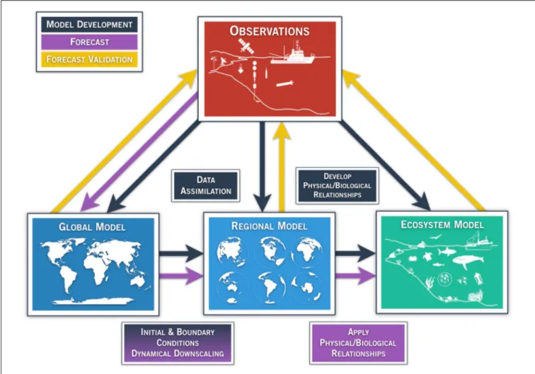
is the forecast time. For accurate predictions, the model needs to be able to capture the key feedbacks within the system of interest that control its time evolution, or trajectory in the model phase space. In one configuration that is becoming widely used, a global climate model is used to force a higher resolution regional circulation model, which in turn forces an ecosystem model (Figure 1). While other forecast systems may take other forms, it can be said generally that in marine ecosystem forecasting, observations (Figure 1, red box) are needed to develop, initialize, and force physical and ecological models on multiple scales (Figure 1, black arrows), to produce a forecast (Figure 1, purple arrows), and finally to validate the forecast (Figure 1, yellow arrows).
In the context of ecosystem-relevant predictions, the model can be a purely physical model at a global or regional scale (Figure 1, blue boxes), if the interest is primarily in the physical ecosystem drivers, or it can be online or offline coupled with an ecosystem model of various levels of complexity (Figure 1, green box). The online coupling strategy consists of running the physical and ecosystem models simultaneously whereas in the offline coupling, the ecosystem model is launched alone. In both strategies, the physical model provides the ecosystem model with the physical variables that are needed for the evolution of the biological quantities. For example, in a simple Nutrient-Phytoplankton-Zooplankton (NPZ) model,
the biological variables will be advected by the model velocity field and diffused according to the physical diffusion coefficients (Franks, 2002). In addition, light and nutrient availability will be controlled by the physical model dynamics. In more complex models, however, light and nutrient availability are controlled by biological processes as well through, for example, phytoplankton absorption and bacterial re-mineralization (Skakala et al., 2018).
Both physical and biological models can either be empirical or dynamical. In the first case relationships among variables are determined from observations using statistical methods, while in the second case the prognostic equations linking the system variables at a given time to their values at a later time are solved numerically. For dynamical models, observations are needed to validate the model, to correct its parameterizations if needed, and identify missing processes (i.e., model development). In operational forecast systems, observations are also used to perform bias-corrections of the forecast in the presence of systematic model errors. The physical models considered in this paper are primarily high-resolution regional ocean models, for which the lateral ocean boundary conditions as well as surface forcing need to be provided. Initial and boundary conditions and surface forcing are obtained from global models, which are themselves constrained by observations through initial conditions and data assimilation.
Depending on the forecasting time scale τ, different observational inputs may be relatively more important. For forecasts up to several months, initial conditions are critical, but the memory of initial conditions is lost at longer lead times, so that boundary conditions and forcing become more important. In addition, observations are essential for validating the skill of the forecast, which includes assessing the reliability and quality of the forecast and refining or constraining forecast uncertainties.
In the following sections we provide examples of a variety of state-of-the-art statistical and dynamical forecasting activities focused on different regions along the North American coasts. These examples illustrate a broad range of approaches that exploit predictability associated with physical processes that are often specific to the different regions considered, and highlight observational needs for the different cases.
Statistical Forecasting Approaches
Linear Inverse Models
In the Linear Inverse Modeling (LIM) framework, the system of interest is described in terms of an anomaly state vector x, which is constructed from anomalies of the key system variables. The evolution of x is then modeled in terms of linearly damped and stochastically perturbed dynamics (Penland and Sardeshmukh, 1995;Newman et al., 2011) of the form:
dx = Lxdt + Sr √
dt, (1)
where the matrix L encapsulates the predictable dynamics of the system, the matrix S represents the amplitude and spatial structure of the stochastic forcing, and r is a vector of random numbers drawn from a normal distribution with zero mean and unit standard deviation. Thus, the first term on the Right-Hand-Side (RHS) of equation (1) describes the changes of
FIGURE 1 | Generalized schematic of a physical-ecological forecast system. Arrows represent techniques for model development (black), ecosystem forecast/prediction (purple), and forecast validation (yellow). Global and regional models (blue boxes) assimilate available observing systems (red box) such as satellite data, tide gauge stations, drifting/moored buoys, profiling floats (e.g., ARGO), gliders, repeated trans-basin sections, regional ship time series, and radar observations. Observations also play a key role in the development of model parameterizations and statistical quantification among the components of the regional and ecosystem (green box) models, as indicated by the black arrow. Output from global models provide initial and boundary conditions for regional models (purple arrow), which dynamically extrapolate the effects of large-scale climate processes to regional or local scales of interest. The choice of the downscaling approach is part of model development (black arrow, shading from black to purple in the lower-left box). In addition, reliable and high-resolution operational observation systems are needed for validating, verifying, and determining the predictive skill of the forecast. Physical/biological relationships are developed based on historical
observations (black box/arrow), and applied in the forecasting step. In the validation step, the output from the forecast system is compared with the appropriate observations (yellow arrows).
the state vector over the small time interval dt associated with deterministic processes, while the second term represents changes due to stochastic forcing as a random walk. The success of equation (1) in describing and predicting the system relies on the large time-scale separation between relatively slow oceanic processes and much faster non-linear atmospheric processes. These fast non-linear processes are represented by the stochastic forcing Sr√dt in equation (1), and their systematic feedbacks on
x, if any, are absorbed in L.
The L operator is estimated directly from the data as to−1ln[C(to)C(0)−1], where C(to) and C(0) are the covariance
matrices of x at the training lag to(chosen to be 3 months) and
at lag 0, respectively. Results are not sensitive to the choice of the training lag provided that the lag is sufficiently long that the noise can be treated as white noise, but shorter than intrinsic
timescales of the system. Having determined L, the stochastic forcing amplitude S can be obtained from the Lyapunov equation:
LC(0) + C(0)LT+SST=0. (2) For a system described by (1) the most likely solution at time t +τ can be determined from the state at time t as:
x(t + τ) = exp(Lτ)x(t) = G(τ)x(t), (3) where G(τ) = exp(Lτ). Equation (3) is used for forecasting applications. The LIM approach has been extensively used to model and predict SST anomalies in the tropical Pacific (Penland
and Sardeshmukh, 1995;Newman and Sardeshmukh, 2017), but
it has also shown skill for the prediction of SST anomalies along the U.S. west coast (Dias et al., 2018, Figure 2). For the
latter application, the Hadley Center Sea Ice and Sea Surface Temperature (HadISST) data were used over the period 1900– 2015. While a LIM constructed using only SST information has proven very useful in many applications, the inclusion in the state vector of information about subsurface ocean dynamics, for example thermocline depth or SSH has improved both modeling and prediction of the tropical Pacific system (Newman et al., 2011;Capotondi and Sardeshmukh, 2015;Capotondi and
Sardeshmukh, 2017; Newman and Sardeshmukh, 2017), and
may improve predictions in other regions. SSH is in itself a very important quantity to predict, given its dynamical link to thermocline depth, as well as its relevance for coastal sea level. The extension of the state vector to other variables (e.g., surface wind stress, ocean currents, sea surface salinity) may further improve the LIM system. An approach similar to the LIM has been successfully used to estimate the potential predictability of Net Primary Production (NPP) and SST over the global ocean, using satellite-based data of the two quantities over the period 1997–2017 (Taboada et al., 2019), although the short duration of the NPP record appeared to severely limit the skill of out-of-sample predictions of the last year of the data. Thus, future LIM applications can be expected to extend existing efforts to improve the modeling and forecasting of biological quantities.
The success of the LIM relies on the ability of the L and
S operators, which are determined from the data, to capture the salient statistical features of the system of interest, which are themselves the expression of the system dynamics. Thus, long, accurate and consistent records of SST, SSH (or other measures of subsurface processes), surface atmospheric forcing (e.g., surface wind stress), and biological quantities are key to the robust determination of the LIM operators, and to the performance of this approach. While century-long SST data sets are now available (albeit with large uncertainties prior to ∼1950), the same is not true for SSH. The latter is usually obtained from reanalysis products, which themselves assimilate SSH observations from satellite altimetry after 1990. Thus, the continuation of the satellite missions providing large-scale SSH observations remains a high-priority for this type of applications. For predictions of SSH along the coast, accurate SSH data are needed for forecast verification. The availability of satellite data that are not contaminated by land, and have been carefully processed (e.g., for tidal removal), is high priority.
Synoptic Meteorology and Coastal Applications
In many studies of ocean-atmosphere interaction, multiple aspects of atmospheric forcing can play a role. An example is coastal sea level, for which atmospheric pressure, circulation, wind stress, storm surges, and wind-induced Ekman transport may all be important (Sweet et al., 2009;Sheridan et al., 2017). One method of analyzing the holistic influence of the atmosphere is through the use of synoptic climatology, more specifically, through atmospheric circulation-pattern identification. Each discrete atmospheric pattern over a region can then be related to an expected set of surface conditions, and their occurrence could be associated with anomalous marine events. Though there have been numerous different methodologies to classify atmospheric
patterns, in recent years one method of classification has become increasingly used: self-organizing maps (SOMs;Sheridan and Lee, 2011), an artificial neural network-based classification technique in which circulation patterns are ordered in a two-dimensional continuum of patterns, with more similar patterns located in closer proximity than more dissimilar patterns. SOMs, generally used with regional fields of sea-level pressure, have been shown to be effective at examining the association between atmospheric circulation and coastal sea-levels (Sheridan et al., 2017), marine ecosystem structure (Kimmel et al., 2009), cold SST events and thermal stress in marine species (Pirhalla et al., 2015), water clarity (Pirhalla et al., 2016), and chlorophyll levels (Sheridan et al., 2013).
Using the synoptic methodology has some limitations, such as that it will not fully capture the most extreme atmospheric events (e.g., hurricanes), due to their atmospheric circulations being effectively ‘unique’ and thus hard to generalize. However, the categorization of the atmosphere into patterns yields substantive statistical power to assess the correlation between the atmosphere and ocean properties. Further, the synoptic methodology serves as an effective statistical downscaling tool for output from weather-forecasting or global-climate models (Schoof, 2013), which in some cases has proven to be superior to finer-scale model-generated atmospheric data (Wetterhall et al., 2009).
The success of this approach relies on the availability of atmospheric and oceanic fields at sufficient temporal and spatial resolution to capture the small-scale variations of interest at synoptic timescales, and of adequate duration to establish reliable statistical relationships between atmospheric and oceanic variables. For example, the analysis of thermal stress of marine species in the western Florida shelf by Pirhalla et al. (2015)
utilized a suite of satellite-based SST products at 9km horizontal resolution covering the period 1982–2012. Similarly, an ongoing study on the influence of weather and climate on biodiversity in the Channel Islands National Marine Sanctuary, CA, uses data at moderate-scale (4km) resolution to analyze cross-shelf SST gradients as a proxy for coastal upwelling (unpublished data).
Global Dynamical Models
Global models, including coupled climate and Earth system models, can capture the dynamic, non-linear interactions of Earth system components and how those interactions express as variability and change in various simulated physical and ecological systems. Relevant to marine ecosystem simulation, Earth System Models are increasingly integrating biogeochemical descriptions and routines that dynamically interact with the physical systems simulated by the model (Dunne et al., 2013;
Hurrel et al., 2013). This model development work increases the relevance of Earth system models for investigating and simulating ecosystem behavior and potentially predicting it.
Because of their ability to represent dynamic physical behavior and system interactions, global models capture modes of variability observed in the climate system as well as projections of those modes onto components of the Earth system, offering predictability on a variety of timescales. For marine ecosystem prediction, the ability of models to accurately forecast physical ecosystem drivers like currents and water
FIGURE 2 | Linear Inverse Model forecasting. Maps of anomaly correlation coefficient (ACC) calculated between the forecasted and the observed SST anomalies in the Northeastern Pacific, as a function of lead time (t) from month-1 (A) to month-12 (L). Forecast was made using a linear inverse model (LIM) built with monthly SST anomalies in the North and Tropical Pacific. Forecast skill was cross-validated: LIM was trained using data from 1900 to 1994 and the forecast was made for the following 20 years, from 1995 to 2015.
temperatures provides foundational information that can be used to understand ecosystem health and expected behavior, especially for target species that are strongly driven by physical environmental factors.
Global climate and Earth system models are routinely used for seasonal prediction at operational prediction centers around the world. Applications of these seasonal prediction systems are diverse, and marine ecosystem prediction efforts have just begun to harness global dynamical seasonal prediction systems for skill. Early efforts in the U.S. have harnessed output from the North American Multi-Model Ensemble (NMME,Kirtman et al., 2014), which includes seven research and operational models from five research and operational centers run in real time on a monthly schedule. The NMME provides a large multi-model ensemble dataset to evaluate and forecast climate variability on seasonal to interannual timescales.
NMME model data is provided at a relatively coarse 1◦×
1◦
resolution, but is useful for capturing large-scale oceanic
variability and drivers of that variability that offer predictability. The NMME’s ability to capture relevant modes of variability has been well-documented (Becker et al., 2014;L’Heureux et al., 2017) and the consistent set of hindcasts offers the opportunity to evaluate the applicability of the system for targeted predictions. In particular, the NMME model output can supply lateral boundary conditions and surface forcing, after proper downscaling, for high-resolution regional forecasting models like those described in Sections “JISAO’s Seasonal Coastal Ocean Prediction of the Ecosystem (J-SCOPE)” and “Bering Sea Modeling and Forecasting.” Only information of physical quantities is provided at present by the NMME system.
An example of a high-resolution, global coupled ocean-biogeochemical model used for operational physical and biogeochemical forecast is the Mercator Ocean Model3. The
Mercator system uses the Nucleus for European Modelling
of the Ocean (NEMO) ocean model4 at 1/12◦
horizontal resolution coupled with a biogeochemical model at 1/4◦
resolution. Many different data sources are assimilated in the model, including, in particular, real time along track sea level anomalies from AVISO5, SST from both remote sensing [e.g.,
the Operational Sea Surface Temperature and Sea Ice Analysis (OSTIA) at daily time resolution, Donlon et al., 2011] and in situ sources, and temperature/salinity profiles from Argo floats. Mercator ocean provides daily forecasts of physical variables and weekly global biogeochemical forecasts. In particular, daily environmental conditions in support of the Tara expedition (section Toward Holistic Marine Ecosystems Monitoring for Improving Ocean Models) were obtained from the real-time output of the Mercator Ocean.
Global Earth System Models of sufficiently high horizontal resolution to realistically capture small-scale ocean circulation features (e.g., eddies and filaments) and their response to climate variations provide invaluable tools for studying physical and biogeochemical coastal processes by seamlessly connecting the small-scale coastal dynamics to the large scale oceanic and atmospheric circulations. However, the initialization and spin-up of global climate models that include biogeochemistry is challenging. Due to the large number of variables in the biogeochemical model relative to the physical model component the spin-up of the model biogeochemistry may require thousands of years (Wunsch and Heimbach, 2008) compared to weeks for the atmosphere and centuries for the ocean and ice components (Stouffer et al., 2004). Also, biogeochemical data are very sparse. Three-dimensional climatology datasets available for biogeochemical initialization exist only for few variables (macro-nutrients, oxygen, dissolved carbon and alkalinity) while data are extremely sparse for other variables, including dissolved organic carbon, dissolved iron, as well as the biomass of various plankton types. As a result, the latter fields are often initialized as constant fields, producing a mismatch with the physical ocean state, and leading to incomplete equilibration in coupled simulations (Seferian et al., 2016). While in regional model configurations empirical algorithms can be used to relate the physical data (e.g., temperature and salinity) to the biogeochemical variables of interest locally (Siedlecki et al., 2015) these empirical relationships may not be applicable at the global scale. Thus, the global expansion of BG-Argo floats would be extremely valuable for providing measurements of biogeochemical quantities to be used for biogeochemical data assimilation and model initialization.
Regional Applications
The U.S. West Coast
Along the U.S. West Coast upwelling is a major driver of ecosystem variability at all timescales. Nutrients upwelled to the sunlit surface layer stimulate blooms of phytoplankton that provide the energy base for the marine food web. Consequently, variability in upwelling intensity and the nutrient content of upwelled waters controls primary production in the California
4https://www.nemo-ocean.eu 5https://www.aviso.altimetry.fr
Current System (CCS) (Jacox et al., 2016). On interannual timescales, the timing and amplitude of the seasonal cycle (phenology) has been shown to have a large impact on ecosystem functioning. The peak upwelling season in the CCS typically occurs during April-July (Garcia-Reyes and Largier, 2012), with disruptions in phenology leading to dramatic changes in ecosystem composition and abundance (e.g., Schwing et al., 2006). In addition to supplying nutrients to the nearshore region, upwelling can also bring low oxygen, corrosive waters to the continental shelf (Feely et al., 2008, 2016; Chan et al., 2017). ENSO and the PDO modulate upwelling at interannual and decadal timescales, respectively, with the former providing a source of seasonal predictability. Downwelling equatorial Kelvin waves that propagate eastward during the development of an El Niño event continue poleward along the western coasts of the Americas as coastally trapped waves, where they deepen the thermocline and contribute to reduced upwelling in those areas, thus providing an oceanic pathway for the ENSO influence on ocean conditions along the west coast of the Americas. In addition, tropical convection associated with equatorial SST anomalies excites atmospheric teleconnections that alter mid-latitude atmospheric circulation, resulting in upwelling that is anomalously weak (strong) during El Niño (La Niña) events. This atmospheric response to ENSO variability is a source of seasonal predictability in the CCS (Jacox et al., 2017), and has important consequences for primary production, fish abundance and species distribution (e.g.,Chavez et al., 2002and references therein). It is important to note that the winds that drive this upwelling have intensified over recent decades, driving the increased presence of corrosive conditions in the CCS (Turi et al., 2016), though future trends in upwelling intensity are likely to be dependent on latitude and season (Rykaczewski et al., 2015). Given the uncertain future of coastal upwelling variability and change, and its impact on the physical, chemical, and biological state of the CCS, it is clear that sustained ocean monitoring of this region is critical.
Oxygen modeling of the Washington and Oregon shelves
Regional models have developed to the point of being able to address process based questions and be compared to observations at high spatial and temporal resolution. For example, modeling work has identified processes that control the spatial variability and timing of hypoxic ocean conditions on Washington and Oregon shelves (Siedlecki et al., 2015). Regions of persistent hypoxia correlated with regions of high respiration in the region, and corresponded to regions previously identified as retentive or recirculation regions. These results were limited to simulations of 2005–2007, but the locations that persistently experienced hypoxia are also present in the climatology of summer conditions from the JISAO’s Seasonal Coastal Ocean Prediction of the Ecosystem (J-SCOPE) simulations spanning 2009–2017, and consistent with recent observations in those regions. The attribution of the respiration process to spatial and temporal variability of hypoxia relied on many levels of observations including subsurface mooring time series, observations of sediment oxygen demand at the sediment-water interface, and benefited from regional observations of rates
for some key ecosystem processes (e.g., respiration, sinking, sediment oxygen demand, zooplankton grazing).
JISAO’s seasonal coastal ocean prediction of the ecosystem (J-SCOPE)
The J-SCOPE model6features dynamical downscaling of regional
ocean conditions in Washington and Oregon waters using a combination of a high-resolution regional model with biogeochemistry and forecasts from NOAA’s Climate Forecast System (CFS). The regional model (ROMS) extends from 43◦
N to 50◦
N with a horizontal resolution of 1.5 km and 40 vertical levels. The CFS fields are interpolated to the regional model grid, and used for lateral boundary conditions of the physical fields, surface forcing and initialization. Lateral boundary conditions of the biogeochemical fields use empirical relationships that relate these fields to salinity. The forecast experiments of J-SCOPE experienced significant biases inherited from some of the CFS variables, highlighting the importance of the global models forecast skill for the performance of the regional forecasting system.
The J-SCOPE forecasts are developed to support the California Current Integrated Ecosystem Assessment. Integrated Ecosystem Assessments (IEAs) are a framework for informing ecosystem-based management, which aims to account for interactions among ecosystem components and managed sectors, as well as cumulative impacts of a wide spectrum of ocean-use sectors (Levin et al., 2009). In the context of the California Current IEA, J-SCOPE provides 6- to 9-month forecasts of ocean conditions that are testable against observations and relevant to management decisions for fisheries, protected species, and ecosystem health. Results will directly inform the IEA process and will forecast indicators requested by the Pacific Fishery Management Council.
Experiments suggest that seasonal forecasting of ocean conditions important for fisheries is possible with the right combination of components, with forecast uncertainty dependent on the variables and specific region of interest. The components that have proved to be critical for the success of the J-SCOPE system include regional predictability on seasonal timescales of the physical environment from a large-scale model, a high-resolution regional model with biogeochemistry that accurately simulates seasonal conditions in hindcast mode (short simulations that incorporate data assimilation), a relationship with local stakeholders, and a real-time observational network, a result that is consistent with an emerging body of literature (Hobday et al., 2016;Tommasi et al., 2017).
J-SCOPE has considerably benefited from the availability of data from anin situ cruise during 2009–2014, as well as bi-weekly measurements of physical and biogeochemical quantities at three moorings located within the model domain. Figure 3 showcases all the observations that have been used to evaluate the model. This has allowed validating both the physical and biogeochemical model components, as well as the model forecasts. In particular, J-SCOPE model performance and predictability were examined for SST, bottom temperature, bottom oxygen, pH, and aragonite
6http://www.nanoos.org/products/j-scope/
FIGURE 3 | Mixed data sources contribute to model initialization and evaluation – J-SCOPE. The J-SCOPE model depends on a series of data sets to continually evaluate the model’s skill. In addition, some of the data sets contribute to regional algorithms that allow the physical data (salinity and temperature) to be extended to oxygen and carbon variables. The data depicted cover different time periods and monitor different suites of variables spanning 2009–2017. The NOAA West Coast Ocean Acidification Cruises (WCOA) are performed every fourth year in the summer upwelling season and provide extensive biogeochemical as well as biological observations in the region. Occupation of the Newport stations, sponsored by NOAA, occurs bi-weekly year-round, and include nutrient, oxygen, biological, and
temperature observations, and occasionally inorganic carbon. The ground fish trawl survey is performed every year by the NOAA Northwest Fisheries Science Center and measures temperature as well as oxygen near the bottom. The moored observations in red are composed mainly of moorings located within NOAA’s Olympic Coast National Marine Sanctuary (OCNMS) that are deployed seasonally. These monitor temperature at the surface and at depth and oxygen at depth. The Chaba mooring (mooring #5), sponsored by the Northwest Association of Networked Ocean Observing Systems (NANOOS), and maintained by the University of Washington, measures temperature, salinity, oxygen, fluorescence, and velocities over the water column and pH at depth; through collaboration with NOAA PMEL, it also monitors carbon dioxide and pH at the surface. The full CCS-wide list of data relevant to ocean acidification and hypoxia is detailed inChan et al. (2016).
saturation state through model hindcasts, forecast (forcing without data assimilation), and re-forecast (forecasts performed on past years) comparisons with observations. Results indicate J-SCOPE forecasts have measurable skill on seasonal timescales (Kaplan et al., 2016; Siedlecki et al., 2016). Bottom ocean conditions (e.g., bottom temperature and bottom oxygen), which are very important for benthic dwelling species, like Dungeness crab, were shown to have more predictability than SST in this region (Siedlecki et al., 2016).
Observations are critical to the development and testing of systems like J-SCOPE. J-SCOPE depends on them in three primary ways: (1) model development and performance evaluation; (2) for constraining initialization and boundary conditions, and (3) for engendering trust with stakeholders and end users through forecast evaluation and uncertainty communication efforts. These observations include regional rate estimates on the lower trophic level ecosystem cycling described in Banas et al. (2009) and Davis et al. (2014), time series from moorings including those operated by NOAA and the OCNMS (Giddings et al., 2014; Siedlecki et al., 2015, 2016), satellite products of SST, SSH and Chlorophyll (Davis et al., 2014;
Giddings et al., 2014), observations taken as part of groundfish surveys performed by NOAA, and water column observations of chemistry performed every few years by NOAA’s OAP and regional projects like PacOOS or the WOAC.
Assessing the physical-biogeochemical response of the California Current System (CCS) to ENSO
While high-resolution regional modeling is an excellent approach to achieve a detailed representation of the physical and biogeochemical coastal processes in the region of interest, it does rely on the availability of lateral boundary conditions and surface forcing fields that are usually provided by global models, and are therefore impacted by those global model biases. The prescription of lateral boundary conditions from global models is especially limiting in regions that are influenced by inflows of remote origin. The CCS is an obvious example. Coastal Kelvin waves excited along the equator during ENSO events enter the domain from the southern boundary of the CCS region, and can produce important modulations of the pycnocline depth in the region. Thus, prescription of biased lateral boundary conditions to a regional CCS model may distort these important influences. In this application, a global high-resolution physical biogeochemical model with a realistic representation of the small-scale features of the CCS was used to assess the response of ocean pH and oxygen, important ecosystem stressors, to ENSO events (Turi et al., 2018).
Findings from this study draw attention to the following: (1) The manifestation of ENSO events in the CCS shows
large variations from event to event. While this diversity can be partly attributed to the diversity of ENSO events in the equatorial Pacific (Capotondi et al., 2015), and the large spread in the atmospheric response to equatorial SST anomalies (Sardeshmukh et al., 2000), due to atmospheric noise, these event-to-event differences do highlight the need for sustained observations of physical
and biogeochemical quantities to monitor the diversity of ENSO influences on the CCS, in the presence of low-frequency natural variability and climate change.
(2) Biogeochemical properties in the surface ocean may respond differently to ENSO than the same properties at depth. For example, as shown in Figure 4, during El Niño events oxygen decreases at the surface, but increases at depth in a narrow band along the coast, while pH shows a similar behavior both at the surface and at depth. Thus, observations spanning the full depth of the water column in this region, and capable of resolving the narrow high variance region along the coast are required to understand the response of these variables to ENSO.
(3) In spite of the extensive observational network in the CCS regions, some biogeochemical data are either not available or sparse, or of insufficient duration to allow the validation of this high-resolution model simulation in this region in a climatological sense. Water column measurements of Dissolved Inorganic Carbon (DIC) and Alkalinity (Alk), which are needed to calculate pH, CO3, and aragonite
saturation, are not regularly measured except from a few locations within the CCS. Surface measurements of pCO2,
which are critical for estimating CO2 flux and validating
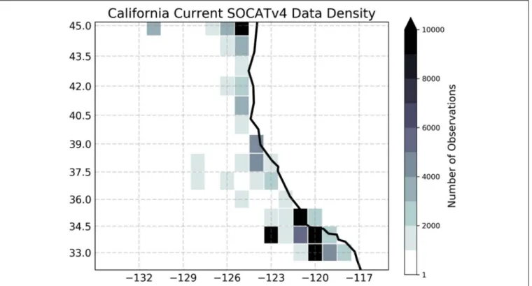
model solutions, are very sparse. Indeed, Figure 5 shows that there are fewer than 3,000 shipboard observations of surface ocean pCO2 over the CCS region during
1982-present. This is a coverage similar to that of the data-poor Southern Ocean region. Finally, water column measurements of O2, which are measured at CalCOFI, are
sparse in large areas of the ocean.
These observational needs are also critical for initializing forecasts in this and other coastal regions.
The Northwest Atlantic
Variability in ocean temperature in the Northwest Atlantic, and in particular in the northeast shelf (NES) is directly linked to two dominant processes: air-sea heat flux, primarily operating on scales of days to months, and ocean advection, operating on scales of months to years. Recent studies demonstrated that an extreme Northeast U.S. warming event observed in 2012 was primarily driven by anomalous wintertime air-sea heat flux, with smaller contributions from ocean advection. However, the relative influence of air-sea heat flux and ocean advection varies from year-to-year (Chen et al., 2014, 2015, 2016). The air-sea heat flux is significantly correlated with the latitude of the atmospheric jet stream, especially in winter and autumn.
Located at the downstream end of an extensive coastal boundary current system, the NES is the direct recipient of cold and fresh water of Arctic origin through accumulated coastal discharge and ice melt that has been advected thousands of kilometers around the boundary of the subpolar North Atlantic. Likewise, subtropical water masses, advected by the Gulf Stream, slope currents, and associated eddies, also influence the composition of water masses within the NES region. The relative strength of the Labrador slope water and warm slope water adjacent to the Gulf Stream have been shown to affect salinity,
FIGURE 4 | ENSO influence on the CCS in a high-resolution global physical-ecosystem model. Composites (warm minus cold) of temperature (A,D) (left panels), O2 (B,E) (middle panels), and pH (C,F) (right panels) at the surface (A–C) (top panels) and at 100 m depth (D–F) (bottom panels) of 6 El Nino and 7 La Nina events during February–March–April from the Geophysical Fluid Dynamics Laboratory (GFDL) Earth System Model version 2.6 (ESM2.6). The composites were computed by averaging each quantity at each model grid point over the 6 El Niño events detected in the 52-year model simulation, and then subtracting the average of the same quantities during the 7 La Niña events present in the simulation. The “warm minus cold” approach was used to increase the signal-to-noise ratio. The model resolution is 0.1◦. Anomalies are standardized by dividing the time series at each grid point by their interannual standard deviation. Notice the difference in the horizontal and vertical spatial structures of different quantities. Temperature and O2anomalies have a broader structure at the surface than at pycnocline depth, while pH anomalies are concentrated near the coast at both depths. Notice how O2anomalies have a different sign at the surface and at depth. These differences in spatial structures suggest the need for monitoring at different depths in the water column to capture property changes. The figure was modified fromTuri et al. (2018)under the Creative Commons Attribution 4.0 License.
nutrients, and temperature on the shelf, as well as zooplankton assemblages and upper trophic level productivity (Green et al., 2013). One of the best leading indicators of the interplay of these two current systems is the latitude of the Gulf Stream (GS) path. Indeed,in situ measurements suggest a direct link between the GS position and the temperature and salinity near the shelf break south of New England (Gawarkiewicz et al., 2012).
Modeling the Northwest Atlantic
The Northwest Atlantic is a highly complex system that sits at the interface of two major current systems, the Gulf Stream and
Labrador Current. Both of these currents highly influence the oceanography of the region as does its complex bathymetry such as the Grand Banks, Georges Bank, and Browns Bank. Therefore, ocean models need to resolve both the regional ocean circulation and complex bathymetry of the region in order to forecast near-term or projected long-near-term ocean conditions (Figure 6).
Both regional and global models have been commonly used to study the physics and biogeochemistry of the Northwest Atlantic. Regional models include ROMS and the Finite Volume Community Ocean Model (FVCOM), both of which have physics-only simulations as well as simulations coupled
FIGURE 5 | Density of in situ observations for the surface ocean partial pressure of carbon dioxide. Shading shows the total number of shipboard measurements in each 1 × 1 degree grid cell between 1982 and 2015, based on the SOCATv4 data set (Bakker et al., 2016). The figure was modified fromBrady et al. (2018)under the Creative Commons Attribution 4.0 License.
with biogeochemical models. These regional ocean models are typically forced by reanalysis data at their ocean boundaries and at their ocean-atmosphere interface, and therefore may suffer from the biases of the forcing fields. Also, as reanalysis data have typically coarser resolutions, they may miss smaller scale features entering the high-resolution model domain. Global climate models participating in the Intergovernmental Panel for Climate Change (IPCC) fourth and fifth assessment reports have also been used to study the oceanography and climate of this region although they are generally limited by their coarse horizontal spatial resolution (∼100 km) in their ocean component. These global models exhibit a persistent bias in the coastal separation point of the Gulf Stream such that the current overshoots and separates from the U.S. east coast too far to the north, leading to very large positive SST bias to the north of the observed Gulf Stream position. However, a prototype high-resolution (∼10 km ocean resolution) global climate model (CM2.6) developed by NOAA’s Geophysical Fluid Dynamics Laboratory (GFDL) shows a reduced bias in the Gulf Stream separation, and is able to resolve the regional circulation and bathymetry of the Northwest Atlantic (Saba et al., 2016). This high-resolution climate model is not a forecasting model but was used to examine the projected changes in the Northwest Atlantic associated with a 1% per year increase in atmospheric CO2over a 70-year period. Results indicate large
temperature increases in the region associated with the CO2
increase, which were not obtained with other GFDL models run at coarser resolutions. Thus, this model has provided very important insights on climate change in the Northwest Atlantic
(Saba et al., 2016). Temperature and salinity measurements in the Gulf of Maine Northeast channel, the major throughway for Slope Waters to enter the shelf at depth (Mountain, 2012) have allowed the model validation at the fine scale of the Channel. This modeling activity has also largely benefited from relatively high-resolution (0.25◦
) NOAA Optimum Interpolation SST (OISST) data (Reynolds et al., 2007) over a long enough period (1981– 2013) to allow the establishment of a reliable SST climatology at the spatial scales relevant for this high-resolution model. Bottom temperature and salinity data from the NOAA Northeast Fisheries Science Center’s fall and spring bottom trawl survey and ecosystem monitoring survey also provided criticalin situ ocean data to estimate model biases.
Temperature predictions in the Northwest Atlantic
The Northwest Atlantic is arguably one of the most dynamic systems in which to explore predictability. In addition to being a temperate system with high seasonality, the coupled Slope Water system causes isotherms to be very close together and their location changes annually due to large-scale oceanographic and atmospheric processes. Because of this spatially and temporally dynamic environment, SST along the Northeast U.S. coast has been shown to have low predictability especially at long time scales (Stock et al., 2015). However, other analyses that have considered subsurface variables indicate the existence of larger predictability in this region. Chen et al. (2016) estimate that the depth-integrated temperature over the NES during winter-spring has a mean decorrelation time scale of ∼50 days, with
FIGURE 6 | Northwest Atlantic Ocean and Labrador Sea bathymetry and major currents. Black arrows indicate colder and fresher water from the Labrador Current, while the white arrows indicate warmer and saltier Slope waters of Gulf Stream origin. Dashed arrows indicate areas where mixing can occur. The inset shows the location of the Northeast Channel (NE Channel) where a mixture of Labrador Current waters and Slope waters enter the Gulf of Maine. The figure was reproduced fromSaba et al. (2016)with permission from AGU.
decorrelation timescales much longer near the bottom than at the sea surface. This mean decorrelation time scale indicates the possibility of some seasonal predictability, and the lead time for skillful predictions may increase when a multivariate system is considered.
As described above, well-established relationships exist between climate aspects of this coupled slopewater system and the local physical quantities that are directly related to the distribution and abundance of zooplankton and fish. Oceanographic features that show some predictability and that relate to ecological endpoints include the Gulf Stream path (Joyce et al., 2000;Nye et al., 2011), coastal sea level (Forsyth et al., 2015), local along-shore wind (Li et al., 2014), atmospheric jet stream latitudes at various longitudes (Chen et al., 2014), PDO (Pershing et al., 2015), and NAO (Joyce et al., 2000;Frankignoul et al., 2001). Activities are underway to relate the temperature in the NES region to various predictands (e.g., Gulf Stream path, along-shore wind etc.) through multiple linear regressions. The skill of this statistical model must be evaluated using observations and/or hindcast and reanalysis products. The determination of the statistical model coefficients, as well as the model validation,
require long time series of both predictands and predictors to allow the establishment of statistically significant relationships.
Bering Sea Modeling and Forecasting
In subarctic regions like the Bering Sea, sea ice and bottom temperature are major drivers and determinants of ecosystem state, with the timing and extent of sea ice cover and open waters influencing the evolution of the seasonal cycle in the region. Date of ice retreat, combined with solar heating and wind mixing determine the timing of the spring bloom on the southern Bering Sea shelf, with early ice retreat favoring late blooms in May or June, and late ice retreat (after March) favoring early phytoplankton blooms (Stabeno et al., 2007). Warm and cold years, as defined by water temperatures between the surface and 70 m depth, correlate to low and high abundance of large zooplankton in the southeastern Bering Sea shelf (Coyle et al., 2011), and the “cold pool,” the area where the bottom temperature is less than 2◦
C, has been found to influence the distribution of major commercial groundfish (Lauth and Kotwicki, 2013). The southern edge of the cold pool itself has shifted ∼230 km north since the early 1980’s (Mueter and Litzow, 2008).
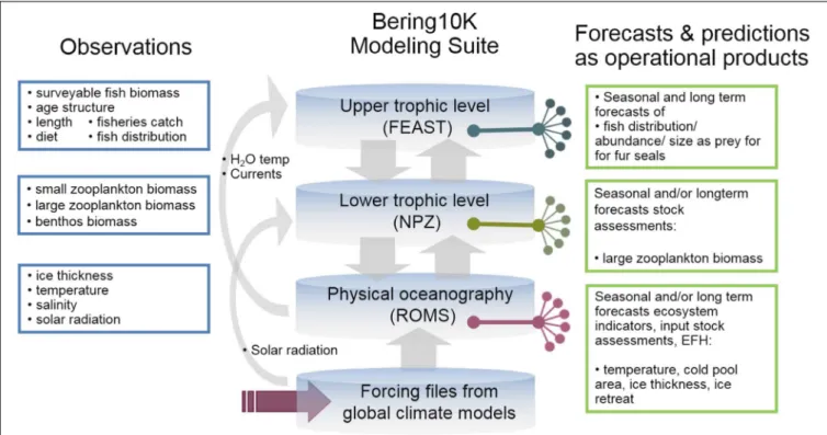
The importance of the Bering Sea region for commercially valuable fish species has stimulated extensive high-resolution modeling efforts in this region. The regional model (named “Bering10k-ROMS”) is based on the Regional Ocean Modeling System (ROMS,Haidvogel et al., 2008) with ∼10 km horizontal resolution and 10 vertical layers. The model domain extends from the western Gulf of Alaska to the Russian coast and to slightly north of the Bering Strait (Figure 7). It is coupled to an ice model and to a lower trophic level NPZ model (known as BESTNPZ,Gibson and Spitz, 2011) with ice-related dynamics and two-way interactions: Bering10k-ROMS feeds ocean currents, temperature and sea ice cover to the NPZ model, which in turn provides phytoplankton density, a quantity that affects attenuation of shortwave radiation and thus heat absorption in the upper water column (Hermann et al., 2013, 2016). The BESTNPZ-Bering 10k-ROMS is additionally coupled to a fish model, the Forage and Euphausiid Abundance in Space and Time (FEAST), which is a 2-dimensional, gridded, daily scaled multispecies length-based foraging, bioenergetics
movement and recruitment model for post larval forage and predatory fish (Ortiz et al., 2016). Together, these models form the Bering10K Modeling Suite (hereafter Bering10K), and were originally designed under the supervision of an ecosystem modeling committee as part of an integrated ecosystem research program, “The Bering Sea Project7,” to
synthesize up-to-date information about the eastern Bering Sea ecosystem and be used both for research and management purposes (Punt et al., 2016). An ocean acidification module has recently been added to the Bering10K modeling suite. For seasonal forecasting using the Bering10K, lateral boundary conditions and surface forcing are provided by the NOAA CFS model.
The Bering10K plays a key role within the region’s work on IEAs8, ecosystem-based fisheries management and strategic
7https://www.nprb.org/bering-sea-project/
8
https://www.integratedecosystemassessment.noaa.gov/regions/alaska/ebs-integrated-modeling
FIGURE 7 | Geographical extent of the Bering10K Modeling Suite showing bathymetry. The primary focus is on the eastern Bering Sea shelf, where in cold years sea ice cover can extend from the Bering Strait to the Alaska Peninsula and retreat in the SE as late as the end of April. The influence of sea ice persists through summer, as cold, dense salty water remains in the bottom as a “cold pool” that typically persists along the middle shelf south of 58◦N.