HAL Id: hal-00947883
https://hal.archives-ouvertes.fr/hal-00947883
Submitted on 20 Mar 2014
HAL is a multi-disciplinary open access
archive for the deposit and dissemination of
sci-entific research documents, whether they are
pub-lished or not. The documents may come from
teaching and research institutions in France or
L’archive ouverte pluridisciplinaire HAL, est
destinée au dépôt et à la diffusion de documents
scientifiques de niveau recherche, publiés ou non,
émanant des établissements d’enseignement et de
recherche français ou étrangers, des laboratoires
Mechanical modeling of helical structures accounting for
translational invariance. Part 1: Static behavior
Ahmed Frikha, Patrice Cartraud, Fabien Treyssede
To cite this version:
Ahmed Frikha, Patrice Cartraud, Fabien Treyssede. Mechanical modeling of helical structures
ac-counting for translational invariance. Part 1: Static behavior. International Journal of Solids and
Structures, Elsevier, 2013, 50 (9), pp.1373-1382. �10.1016/j.ijsolstr.2013.01.010�. �hal-00947883�
Mechanical modeling of helical structures accounting
for translational invariance. Part 1: Static behavior
Ahmed Frikhaa, Patrice Cartraudb, Fabien Treyss`edea,∗
aLUNAM Universit´e, IFSTTAR, MACS, F-44344 Bouguenais, France b
LUNAM Universit´e, GeM, UMR CNRS 6183, Ecole Centrale de Nantes, 1 rue de la No¨e, 44 321 Nantes C´edex 3, France
Abstract
The purpose of this paper is to investigate the static behavior of helical structures under axial loads. Taking into account their translational invariance, the homogenization theory is applied. This approach, based on asymptotic expansion, gives the first-order approximation of the 3D elasticity problem from the solution of a 2D microscopic problem posed on the cross-section and a 1D macroscopic problem, which turns out to be a Navier-Bernoulli-Saint-Venant beam problem. By contrast with earlier references in which a reduced 3D model was built on a slice of the helical structure, the contribution of this paper is to propose a 2D microscopic model. Homogenization is first applied to helical single wire structures, i.e. helical springs. Next, axial elastic properties of a seven-wire strand are computed. The approach is validated through comparison with reference results: analytical solution for helical single wire structures and 3D detailed finite element solution for seven-wire strands.
Keywords: Homogenization; Helical coordinates; Finite element method; Helical springs; Seven-wire strands; Axial load.
1. Introduction
Helical structures are widely used in mechanical and civil engineering appli-cations. These structures are usually subjected to large loads which can lead
∗Corresponding author
to the material degradation and cracks associated with corrosion and mechan-ical fatigue. This threatens the structural strength. In this framework, non-destructive testing is a crucial tool for detection, localisation and measurement of material discontinuities. The choice of the appropriate technique depends on dimensions and accessibility of the structure. Particularly, ultrasonics allow to control large components, such as plates and tubes, by analyzing their elastic guided waves. The purpose of this study, which is composed of two parts, is to develop a numerical model for the analysis of the elastic wave propagation phenomenon in prestressed helical structures. This problem requires the com-putation of the static prestress state. Therefore, a first model will be developed in Part 1 of this paper, to compute this static state. Taking into account this prestress state, a second model will be developed in Part 2, in order to analyze the wave propagation in these prestressed structures. The goal of this first part of this paper is thus to develop an approach that allows the computation of the prestress state in helical structures subjected to axial load.
Numerous works have been devoted to the modeling of the static behavior of helical structures as springs and multi-wire cables under axial loads. For helical springs, an analytical model was proposed among others in Ancker and Goodier (1958) and Wahl (1963) considering the spring as an Euler-Bernoulli beam with pitch and curvature corrections. Numerical approaches describing the static behavior of helical springs have been also developed. Among these works, a finite element model of half of a spring slice has been proposed in Jiang and Henshall (2000).
The static behavior of seven-wire strands has been widely studied in lit-erature. Various analytical models based on different assumptions have been proposed, such as the model of Costello (1977) which is one of the most popu-lar. These models are reviewed in Jolicoeur and Cardou (1991) and compared in Jolicoeur and Cardou (1991) and Ghoreishi et al. (2007). Besides, numerical models relying on the finite element method were developed. Some of them are based on beam elements (Durville (1998); Nawrocki and Labrosse (2000); P´aczelt and Beleznai (2011)), see also Nemov et al. (2010) and Bajas et al.
(2010) in which ITER superconducting cables composed of a large number of strands are studied. But most of the time, 3D models are used, see e.g. Boso et al. (2006), Ghoreishi et al. (2007), ˙Imrak and Erd¨onmez (2010), Nemov et al. (2010), Stanova et al. (2011a,b), Erd¨onmez and ˙Imrak (2011). In order to ob-tain a good representation of the geometry as well as the displacement solution, which may involve bending phenomena, quadratic elements are employed. This leads to models which can be computationally expensive, when the model axial length is about the pitch length. Therefore, as soon as the loading fulfills helical symmetry, one can take benefit of this property to reduce the model size. This has been achieved in Jiang et al. (1999, 2008) in which the computational do-main is restricted to a basic sector of a helical slice. Helical symmetry may also be accounted for within the framework of homogenization theory. This has been proposed first in Cartraud and Messager (2006) using axial periodicity, and then improved in Messager and Cartraud (2008), in which helical symmetry enables to consider one slice of a strand. The derivation of the slice model is different in Jiang et al. (1999, 2008) and Messager and Cartraud (2008). However, in both cases, helical symmetry yields displacement constraints between the two faces of the slice, with a loading under the form of an axial strain and a twist rate.
This work further advances Cartraud and Messager (2006) and Messager and Cartraud (2008), taking advantage of the translational invariance. Helical symmetry can be actually considered more efficiently. Thus the model can be reduced to a 2D one, i.e. a cross-section model. This requires to formulate the homogenization theory in a twisted coordinate system. This technique then allows the computation of the static prestressed state of helical structures (single wire and multi-wire) from the solution of a 2D problem. Let us mention that an advanced analytical 2D model has been recently proposed in Argatov (2011). This model takes into account Poisson’s effect, contact deformation and allows to obtain the overall strand stiffness as well as local contact stresses. In this reference, plane strain was assumed to formulate the 2D problem while in the present work helical symmetry is used.
struc-tures composed of a stack of helical wires wrapped with the same twisting rate around a straight axis. As explained in Section 3, this excludes the case of double helical structures (such as independent wire rope core for instance) and cross-lay strands.
This paper is organized as follows. First, in Section 2, the curvilinear coor-dinate system is introduced. Then in Section 3 the translational invariance is defined, which is a necessary condition for the helical homogenization approach. Based on the asymptotic expansion method and exploiting the translational invariance property, the homogenization procedure is presented in Section 4. Its finite element solution is detailed in Section 5. The helical homogeniza-tion approach is validated for helical single wire and seven-wire structures by comparison with analytical or numerical models in Section 6.
2. Curvilinear coordinate system
A helical structure is considered (see Fig.1). Let (eX, eY, eZ) its Cartesian
orthonormal basis. The helix centreline is defined by its helix radius R in the Cartesian plane (eX, eY) and the length of one helix pitch along the Z-axis
denoted by L. This helix centerline can be described by the following position vector: r(s) = R cos(2π l s + θ)eX+ R sin( 2π l s + θ)eY + L lseZ, (1) where l =√L2+ 4π2R2is the curvilinear length of one helix pitch and θ is the
helix phase angle in the Z = 0 plane. For a seven-wire strand, θ is equal to (N − 1)π/3, where N = 1, .., 6 refers to the number of the helical wire. θ is equal to zero for a single wire helical structure. The helix lay angle Φ is defined by tanΦ = 2πR/L. A complete helix is described by the parameter s varying from 0 to l.
2.1. Serret-Frenet basis
A Serret-Frenet basis (en, eb, et) associated to the helix can be defined (see
den/ds = τ eb− κet and deb/ds = −τen. For helical curves, the curvature
κ = 4π2R/l2 and the torsion τ = 2πL/l2 are constant. In the Cartesian basis,
en, eb and etare expressed by:
en = − cos( 2π l s + θ)eX− sin( 2π l s + θ)eY , eb= L l sin( 2π l s + θ)eX− L l cos( 2π l s + θ)eY + 2π l ReZ , et= − 2πR l sin( 2π l s + θ)eX+ 2πR l cos( 2π l s + θ)eY + L leZ. (2)
The normal vector en remains parallel to the (eX, eY) plane while eb and et
move in the three directions of the Cartesian basis as s and θ vary.
2.2. Twisted basis
A special case of the Serret-Frenet basis denoted by (ex, ey, eZ)
correspond-ing to κ = 0 and τ = 2π/L can be considered. It corresponds to a twisted coordinate system along the Z-axis (s ≡ Z) with axial periodicity L. The unit vectors exand ey rotate around the Z-axis and remain parallel to the (eX, eY)
plane (see Fig. 1). In the Cartesian basis, ex and ey are expressed as:
ex= − cos( 2π LZ + θ)eX− sin( 2π LZ + θ)eY , ey= sin( 2π LZ + θ)eX− cos( 2π LZ + θ)eY. (3)
It should also be noted that this twisted coordinate system coincides with the one proposed in Onipede and Dong (1996), Nicolet et al. (2004), Nicolet and Zola (2007) for the analysis of twisted and helical structures.
2.3. Covariant and contravariant bases
Differential operators can not be expressed directly in the Serret-Frenet or twisted bases. They have first to be expressed in the covariant and contravariant bases. The reader can find an in-depth treatment of curvilinear coordinate sys-tems in Chapelle and Bathe (2003), Synge and Schild (1978), Wempner (1981) for instance.
e x e Z (x,y) Z e Z e X e Y O L R e X e Y Z=s=0 Z=s=0 s=l e y Z=L e x e y
Figure 1: Left: One helix pitch and its twisted basis associated to the twisted coordinate system (x, y, Z). Right: view normal to the Z-axis. The point Z = s = 0 lies in the (eX, eY)
plane.
From the twisted basis (ex, ey, eZ), a new coordinate system (x, y, Z) is built,
for which any position vector can be expressed as:
X(x, y, Z) = xex(Z) + yey(Z) + ZeZ. (4)
The covariant basis (g1, g2, g3) is obtained from the position vector by (g1, g2, g3) =
(∂X/∂x, ∂X/∂y, ∂X/∂Z), which yields in the twisted basis:
g1= ex(Z) , g2= ey(Z) ,
g3= −τyex(Z) + τ xey(Z) + eZ.
(5)
Note that the covariant basis is not orthogonal.
The covariant metric tensor, defined by gmn= gm· gn, is then given by:
g= 1 0 −τy 0 1 τ x −τy τx τ2(x2+ y2) + 1 . (6)
The covariant basis gives rise to the contravariant one (g1, g2, g3), defined from
gi·gj = δij. Superscripts and subscripts refer to the covariant and contravariant vectors, respectively. g1, g2and g3 are expressed in the twisted basis as:
g1= ex(Z) + τ yeZ , g2= ey(Z) − τxeZ , g3= eZ. (7)
The Christoffel symbol of the second kind Γk
ij, defined by Γijk = gi,j· gk, can
be calculated from the covariant and contravariant bases, which leads to:
Γk 11= Γ12k = Γ21k = Γ22k = 0, Γ1 13= Γ 1 31= 0, Γ 1 23= Γ 1 32= −τ, Γ 1 33= −τ 2x, Γ2 23= Γ 2 32= 0, Γ 2 33= −τ 2y, Γ2 13= Γ 2 31= τ, Γ3 13= Γ 3 31= Γ 3 23= Γ 3 32= Γ 3 33= 0. (8)
It is noteworthy that the coefficients Γk
ij do not depend on the axial variable
Z. As shown in the next section, this is a necessary condition for translational invariance.
2.4. Strain tensor
The strain tensor is now rewritten in the curvilinear coordinate system. In the contravariant basis, the strain-displacement relation is (Chapelle and Bathe (2003)): ǫ= ǫijgi⊗ gj , ǫij = 1 2(ui,j+ uj,i) − Γ k ijuk, (9)
where the ui’s denote the displacement covariant components.
Using the relation (7) between the contravariant and the twisted bases, the strain vector can then be expressed in the twisted basis as follows:
{ǫ} = (Lxy+ LZ ∂ ∂Z){u}, Lxy= ∂/∂x 0 0 0 ∂/∂y 0 0 0 Λ ∂/∂y ∂/∂x 0 Λ −τ ∂/∂x τ Λ ∂/∂y , LZ = 0 0 0 0 0 0 0 0 1 0 0 0 1 0 0 0 1 0 , (10)
where Λ = τ (y∂/∂x − x∂/∂y). The column vectors {u} = [uxuyuZ]T and
{ǫ} = [ǫxxǫyyǫZZ2ǫxy2ǫxZ2ǫyZ]T are the displacement vector and the strain
vector respectively, both written in the orthonormal twisted basis (ex, ey, eZ).
2.5. Constitutive law
For an isotropic material, the elasticity tensor is given in the covariant basis by (Chapelle and Bathe (2003)):
C= Cijklgi⊗ gj⊗ gk⊗ gl, Cijkl= νE (1 + ν)(1 − 2ν)g ijgkl+ E 2(1 + ν)(g ikgjl+ gilgjk), (11)
where E and ν are the Young modulus and the Poisson’s ratio, respectively. Using the relation between the covariant and the twisted bases and after simpli-fications, it can be checked that the elasticity tensor components in the twisted basis are given by:
Cαβδγ =
νE
(1 + ν)(1 − 2ν)δαβδδγ+ E
2(1 + ν)(δαδδβγ+ δαγδβδ), (12) where greek subscripts {α, β, γ, δ} denote components x, y, Z in the twisted basis. The above expression coincides with the one obtained in the Cartesian basis, as the twisted basis is orthonormal.
3. Translational invariance
Translational invariance is a key property for applying the homogenization theory. For cylindrical structures, translational invariance means that both the cross-section and the material properties do not vary along the axis. For curved structures, there is another condition which states that the differential operator coefficients must not depend on the axial variable (Treyss`ede (2011)). As a consequence, for helical structures, the translational invariance requires the following three conditions (Treyss`ede (2008), Treyss`ede and Laguerre (2010)):
1. The material properties do not vary along the Z-axis in the twisted coordinate system;
2. The coefficients of the differential operators (gradient, divergence, Lapla-cian, ...) are independent on the axial variable Z;
3. The cross-section does not vary along the Z-axis in the twisted coordinate system.
Throughout this work, the material is assumed to be homogeneous and isotropic. In this case, the first condition is verified. To satisfy the second condition, it is sufficient to prove that the Christoffel symbols do not depend on the axial variable Z, which has been verified in the last section (see Eq. 8). Thus it remains only to verify the third condition.
Let us consider a helical single wire structure. The cross-section shape in the (eX, eY) plane at the axial position Z1 is similar to that given at the position
Z2: there only exists a rotation of angle 2π(Z2 − Z1)/L around the Z-axis
between these two cross-section shapes. Moreover, because the twisted basis plane (ex, ey) also rotates around Z, the cross-section indeed remains fixed in
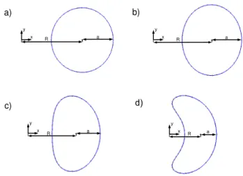
this plane. Therefore, the translational invariance is checked for helical single wire structures. Fig. 2 shows the cross-section of four helical single wires with R = 2a and different helical angles in the (eX, eY) plane. a is the radius of the
circular cross-section (the cross-section being circular in the plane normal to the helical curve). Note that for small angle Φ, the cross-section shape in this plane is nearly circular because the structure is close to a cylinder (Fig. 2a). However the cross-section shape deviates from the circular one as Φ increases.
Let us now consider multi-wire helical structures. They are composed of a stack of helical wires, wrapped around a straight wire. A seven-wire strand is a special case of helical multi-wire structures containing one layer of six helical wires wrapped around the central wire. In the twisted basis, a cylindrical struc-ture of axis Z with isotropic material is translationally invariant for any value of the torsion τ (see Treyss`ede and Laguerre (2010)). It therefore remains fixed in the Cartesian as in the twisted coordinate systems. The central wire is hence translationally invariant. As shown for helical single wire, the peripheral helical wires, which have the same helix parameters are also translationally invariant in the twisted coordinate system. The geometric invariance is then verified
d)
x
R a
y
Figure 2: Cross-section of helical wires, R/a = 2 and (a) Φ = 10◦, (b) Φ = 30◦, (c) Φ = 50◦,
(d) Φ = 70◦.
for the seven-wire strand in the twisted coordinate system and the problem is translationally invariant.
Let us briefly examine more complex structures. In multi-layer wire ropes, more than one layer of helical wires is present. Translational invariance in such structures is still satisfied if the torsion of each wire remains identical. This implies that translational invariance is not fulfilled in case of cross-lay strands because the torsion can be positive or negative. This loss of invariance is obvious if one thinks of contact discontinuities between two layers of opposite torsion. Contact discontinuities also necessarily occur in double helical structures, com-posed of one central strand wrapped by several peripheral strands. Such double helical structures, sometimes referred to as IWRC (independent wire rope core), hence cannot fulfill translational invariance.
To conclude this section, let us define the cross-section boundary in the plane Z = 0. The surface boundary of a helical single wire with circular cross-section is described in the Serret-Frenet basis by the following position vector:
X(x, y, s) = r(s) + a cos ten(s) + a sin teb(s), (13)
parameterization in the (eX, eY) plane is:
X(t) = (R − a cos t) cos(ηa sin t + θ)+ L
la sin t sin(ηa sin t + θ) Y (t) = (R − a cos t) sin(ηa sin t + θ)+
L
la sin t cos(ηa sin t + θ)
, (14)
where η = −4π2R/lL. This curve has been used to plot the cross-sections on
Fig. 2. It has also been used for the FE mesh generation in Section 6.
4. Helical homogenization procedure
In this work, helical structures are supposed to be subjected to external loads at its end sections. Moreover, only axial loads (traction and torsion) are considered. Targeted helical structures are helical springs and seven-wire strands.
As explained in introduction, the purpose of this paper is to propose an ap-proach for obtaining the static stress state, which will be used in the second part of this paper as a prestress state, for a wave propagation analysis. This can be achieved efficiently using an homogenization method. This approach, based on the asymptotic expansion method, exploits the translational invariance prop-erty. Homogenization splits the initial 3D elasticity problem into 2D problems posed on the cross-section, and a 1D straight beam problem. The overall beam behavior is computed thanks to the solution of the 2D problems. This solution, combined with the solution of the beam problem, provides also the local stress state.
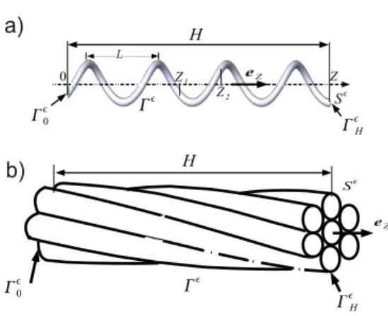
For the present work, let us consider a slender helical structure of axial length H (see Fig. 3), with a cross-section denoted Sε. This structure occupies
the configuration Ωε = Sε× [0, H]. The boundary of Ωε is defined by ∂Ωε =
Γε∪Γε
0∪ΓεH, with Γε0= Sε×{0} and ΓεH= Sε×{H} the two end cross-sections of
the helical structure and Γεthe cross-section boundary. This structure exhibits
a small parameter ε, corresponding to the inverse of the slenderness ratio, i.e. the ratio between the diameter of the cross-section Sε and the length H.
a) H eZ S H 0 b) H H 0 Z1 Z2 0 Z
Figure 3: 3D helical structures. (a) single wire, (b) seven-wire strand.
4.1. The initial problem
The linear elasticity problem consists in finding the fields σε, ǫε and uε,
solution of: ∇ · σε= 0 σε= C : ǫε(uε) ǫε(uε) = ∇s(uε) σε· n = 0 on Γε , (15)
where C is the elasticity tensor, which is supposed to be constant under the assumption of small displacements. ∇s(·) and ∇ · (·) denote respectively the
symmetric gradient (strain) and divergence operators. The solution must also verify the boundary conditions at the end sections. They are supposed to be under the form of stress data: σε· (−e
Z) = t0 on Γε0and σε· eZ = tH on ΓεH,
where t0 and tH are the tractions at the end sections located at Z = 0 and
Z = H. Moreover t0 and tH are such that the overall structure equilibrium is
fulfilled, which is a necessary condition for problem (15) to have a solution. For seven-wire strand, the solution must verify Eq. (15) on each wire as well as contact equations, on the contact line between the central wire and each helical wire. This raises the problem of contact assumptions. In Ghoreishi et al. (2007), stick and slip conditions have been studied for computing the overall behavior. In Gnanavel and Parthasarathy (2011), an analytical model with
frictional contact was developed. Overall stiffness as well as maximum normal contact stresses were calculated from the authors’s model and the Costello’s model which assumes stick contact. In Argatov (2011) hypothesis of slip con-tact is made and maximum concon-tact pressures (core-wire and wire-wire) were compared to FE computations performed with frictional contact in Jiang et al. (2008). All of these previous works have shown that the overall stiffness and contact stresses are very little sensitive to contact conditions. Therefore in this work, for simplicity, the contact is assumed to be stick. This amounts to perfect bonding conditions between wires: uc= up and (σ · n)+c + (σ · n)−p = 0, where
the subscripts c and p are related to the central and peripheral wires.
The solution of this problem (15) with boundary conditions and contact equations for multi-wire strand provides the prestress state. As mentioned pre-viously, this problem may be computationally expensive to solve under this form, and the homogenization method aims to simplify it.
4.2. Asymptotic expansion method
To our knowledge very few works have been devoted to the asymptotic analy-sis of helical structures starting from a 3D formulation. We just mention Nicolet et al. (2007) in the framework of electrostatics. Therefore, the approach pre-sented in this paper is based on Buannic and Cartraud (2000) and Buannic and Cartraud (2001a) developed for axially invariant and periodic beam-like structures respectively. More about asymptotic expansion method for slender structures may be found in some books (Sanchez-Hubert and Sanchez-Palencia (1992); Kalamkarov and Kolpakov (1997); Trabucho and Via˜no (1996)).
The first step of the method consists in defining a problem equivalent to problem (15), but posed on a fixed domain that does not depend on the small pa-rameter ε. A change of variables is thus introduced which takes into account the structure slenderness, in the twisted coordinates system: (x, y, ζ) = (x, y, εZ). ζ = εZ denotes the slow scale or macroscopic 1D-variable and {x, y} denote the fast scale or microscopic 2D-variables. According to this change of variables,
the differential operators become ∇s(.) = ∇s xy(.) + ε∇sζ(.) , ∇ · (.) = ∇xy· (.) + ε∇ζ · (.) , (16) where ∇s
ζ(.) and ∇ζ · (.) correspond to partial differentiations with respect to
the macroscopic variable ζ. ∇s
xy(.) and ∇sxy·(.) denote the differential operators
with respect to the microscopic variables x and y.
Next, the displacement solution is searched under an asymptotic expansion form:
u(x) = u0
x(ζ)ex+ u0y(ζ)ey+ εu1(x, y, ζ) + ε2u2(x, y, ζ) + ... (17)
In this expression, the translational invariance is taken into account since the kth-order displacement uk(x, y, ζ) does not depend on the microscopic axial
coordinate Z. Moreover, it is usually considered that the 0th-order
displace-ment has no axial component, which results from the property that for slender structures, the bending stiffness is much lower than axial stiffness. So 0th-order
displacement corresponds to a transverse deflection. Note that a proof of this result may be found in Trabucho and Via˜no (1996) for homogeneous beams, and in Kolpakov (1991) for beams with periodic structure. As axial loads are considered in this work, and under the assumption that bending is not coupled with tension and torsion, this 0th-order term vanishes.
Reporting expansion (17) in problem (15) with the use of (16), and con-sidering ζ and {x, y} as independent coordinates, one is led to a sequence of problems. On one hand 2D microscopic problems posed on the cross-section S, which will be denoted Pm
2D, where m denotes the order of ε in the equilibrium
equation. On the other hand a sequence of 1D macroscopic problems will be also obtained, but only the lowest order macroscopic problem will be considered in the following.
4.3. Microscopic problems
The lowest order 2D microscopic problem posed on the cross-section S is P1
2D with the following equations:
∇xy· σ1= 0 σ1= C : ǫ1 ǫ1= ∇sxy(u1) σ1· n = 0 on ∂S . (18)
It is important to notice that though this problem is 2D, the displacement u1
has three components. This results from the property than in a matrix form, from Eq. (10), one has:
{∇sxy(u1)} = Lxy{u1} = Lxy u1 x u1 y u1 ζ . (19) Problem P1
2Dis well-posed and has a unique solution up to a rigid body motion
(Sanchez-Hubert and Sanchez-Palencia (1992); Buannic and Cartraud (2000)). The stress solution is obviously equal to zero. The displacement is thus a rigid body motion solution of ∇s
xy(u1) = 0, its expression in the twisted basis is:
u1= u1
ζ(ζ)eZ+ ϕ1(ζ)[xey− yex], (20)
corresponding to an overall translation u1
ζ and rotation ϕ1 around the Z-axis.
The solution of problem (18) is then given by u1 with at this step arbitrary
u1
ζ(ζ) and ϕ1(ζ) and ǫ1= σ1= 0.
The next order microscopic problem P2
2Dinvolves σ2, ǫ2 and u2solution of:
∇xy· σ2= 0 σ2= C : ǫ2 ǫ2= ∇sxy(u2) + ∇sζ(u1) σ2· n = 0 on ∂S . (21)
Note that the displacement vector u1, obtained from the solution of the
problem P1
that the components of this strain tensor are, under a matrix form: {∇sζ(u1)} = h 0 0 EE 0 −yET xET iT, (22) where EE = ∂u1 ζ/∂ζ and ET = ∂ϕ
1/∂ζ and thus can be identified as
macro-scopic strains, i.e. extension and torsion respectively. Therefore, the other part of the strain ∇s
xy(u2) is a microscopic strain.
Thanks to the problem linearity, its solution is a linear function of the macro-scopic strains, up to a rigid body displacement which is of the form (20). So one has: u2= χE(x, y)EE(ζ) + χT(x, y)ET(ζ)+ u2 ζ(ζ)eZ+ ϕ2(ζ)[xey− yex] , σ2= σE(x, y)EE+ σT(x, y)ET . (23)
As it will be shown in the next section, the lowest order macroscopic problem is a 1D beam problem, with extension and torsion. It thus involves macroscopic beam stresses which are simply defined from the integration over the cross-section S of the local or microscopic stresses σ1. Consequently the axial force
T and the torque M take the form:
T (ζ) =R Sσ 2 ζζdS , M (ζ) =R S(−yσ 2 xζ+ xσ 2 yζ)dS , (24)
and from the solution of problem (21), one can define the overall beam behavior such that: T M = [khom] EE ET , (25)
where [khom] is the stiffness matrix, which is symmetric.
4.4. Macroscopic problem
The lowest order macroscopic problem can be derived from compatibility conditions which express that problem (21) admits a solution, see e.g. Buannic and Cartraud (2000, 2001a). It amounts to integrate equilibrium equations of
problem (21) over the cross-section. This yields: dT /dζ = 0 dM /dζ = 0 T M = [khom] EE ET EE= ∂u1 ζ/∂ζ ET = ∂ϕ1/∂ζ , (26)
with boundary conditions at ζ = 0 and ζ = εH. Since we have stress data for the 3D initial problem, and taking into account the overall equilibrium, these boundary conditions can be written as:
T (0) =R St 0· (−e Z)dS M (0) =R S(yt 0 · ex− xt0· ey)dS T (εH) = T (0) M (εH) = M (0) , (27)
which corresponds to the application of the Saint-Venant principle, rigorously justified in the framework of asymptotic analysis of beams in Buannic and Car-traud (2001b).
The solution of this 1D macroscopic problem (26-27) is thus straightforward with a uniform macroscopic state: T = T (0), M = M (0), with the macroscopic strains EEand ET obtained from the inversion of (25) and u1
ζ and ϕ1calculated
thanks to (26)4−5 and defined up to a constant.
4.5. Summary
One can summarize the results of the asymptotic expansion method with the following expressions:
u(x) = ε(u1
ζ(ζ)eZ+ ϕ1(ζ)[xey− yex])+
ε2(χE(x, y)EE+ χT(x, y)ET+
u2
ζ(ζ)eZ+ ϕ2(ζ)[xey− yex]) + O(ε3) ,
σ= ε(σE(x, y)EE+ σT(x, y)ET) + O(ε2) .
It is recalled that microscopic fields χE(x, y), χT(x, y), σE(x, y) σT(x, y) are
provided by the solution of the 2D microscopic problem (21) posed on the cross-section. Then, the expansions given in (28) can be easily computed up to the second-order rigid body motion, combining the previous solution of the 1D macroscopic problem with these microscopic fields.
5. Finite element solution
The variational formulation of the 2D microscopic problem (21) in the twisted coordinate system takes the form:
∀δu2(x, y),
Z
S∇ s
xy(δu2) : σ2dxdy = 0, (29)
and from Eq. (21)3:
σ2= C : (∇sxy(u2) + ǫmacro), (30)
with ǫmacro= ∇sζ(u1). Hence one has:
∀δu2(x, y), Z S∇ s xy(δu2) : C : ∇sxy(u2)dxdy = − Z S∇ s
xy(δu2) : C : ǫmacrodxdy.
(31)
We recall that {∇s
xy(u2)} = Lxy{u2}, see (19). Then a finite element
approx-imation of the form {u2
} = [Ne]{Ue} is introduced , where [Ne] is the matrix
of shape functions, and {Ue} the nodal displacements, with three degrees of
freedom at each node. The variational formulation yields:
[K]{U} = {F }, [Ke] = Z Se [Ne]TLT xy[C]Lxy[Ne]dxdy, {Fe} = − Z Se [Ne]TLT xy[C]{ǫmacro}dxdy, (32)
with [K] the stiffness matrix obtained from the assembly of element stiffness matrices [Ke].
Note that in (32) the external load is given under the form of a macroscopic strain {ǫmacro}.
Once this system is solved, the stresses are computed thanks to (30) and after integration over the cross-section, the macroscopic beam stresses, i.e. the axial force and the torque are computed, thus providing the overall behavior [khom].
6. Validation of the homogenization approach
In this section, the microscopic response is computed for helical springs and seven-wire strands under axial loading. The 2D FE model based on helical homogenization has been implemented in an in-house code. This model is first validated for helical springs by comparison with an analytical solution. Another validation is also presented for seven-wire strands with a reference solution ob-tained from a 3D FE model.
For helical single wire or multi-wire structures subjected to a given macro-scopic extension EE (ET = 0), first the 2D model is generated. The
cross-section is meshed, with six-node triangle elements to improve the geometrical description as well as results accuracy. The solution of the microscopic 2D prob-lem is defined up to a rigid body displacement in the twisted coordinate system, see Eq. (20), which can be fixed by prescribing the axial displacement uZ of an
arbitrary node and the binormal displacement uy of a node on the line y = 0.
Then Eq. (32) is solved, and in the post-processing step, the computation of the axial force T and moment M are performed as well as the overall behavior.
6.1. Helical single wire structures
A helical single wire structure with circular cross-section is studied. R, Φ, n and a denote the helix radius, helix angle, number of helix pitches and the wire radius, respectively. Two types of structures can be distinguished: helical springs (large helix angle Φ and ratio R/a) and civil engineering cable (small angle Φ). The homogenization approach proposed in this paper is valid for any type of helical structures. However, in the literature, analytical solution is available only in the case of helical spring. Therefore, the validation of the homogenization approach is performed in that case.
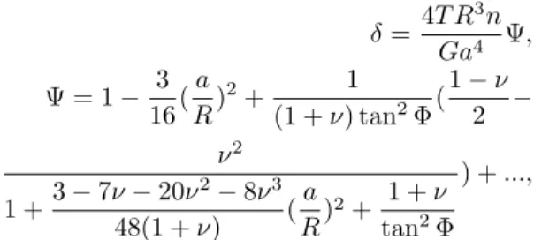
The analytical solution may be found in Ancker and Goodier (1958). When one end-section is clamped while the other is subjected to axial load T with a fixed rotation, the axial deflection δ at its end is given by:
δ = 4T R 3n Ga4 Ψ, Ψ = 1 − 3 16( a R) 2+ 1 (1 + ν) tan2Φ( 1 − ν 2 − ν2 1 +3 − 7ν − 20ν 2 − 8ν3 48(1 + ν) ( a R) 2+ 1 + ν tan2Φ ) + ..., (33)
where Ψ is a pitch and curvature correction factor.
Figure 4: Correction factor Ψ vs. a/R for Φ = 70◦, 75◦, 80◦, 85◦.
The inputs of the analytical solution are the ratio a/R, the helix angle Φ and the Poisson coefficient ν. For given geometric and material parameters, Eq. (33) is used to compute the correction factor Ψ.
The numerical results provided by the homogenization approach are com-pared with the analytical solutions for helical springs as follows. For a given δ, the macroscopic strain EE = δ/nL, ET = 0 is imposed as the loading in
to a numerical value of Ψ according to Eq. (33)1, which is compared to the
analytical solution given by Eq. (33)2. For ν = 0.3, Fig. 4 shows the variation
of the correction factor Ψ as a function of a/R for helix angle Φ = 70◦, 75◦, 80◦
and 85◦. Only small differences between numerical and analytical results can
be seen for a/R ≤ 0.2. This difference increases with a/R and as Φ decreases but remains less than 0.7% for Φ = 70◦ and a/R = 0.35, which is small.
The same evolution of the differences between the numerical results and the analytical solution was observed in Jiang et al. (2008), using a 3D FE model, with a free rotation. They are due to the non validity of the analytical model for large a/R and small helix angle Φ. However, our numerical results are in good agreement with those obtained from the analytical model providing a first validation of the computational homogenization approach.
Figure 5: Dimensionless microscopic displacements in the cross-section of a helical spring (R/a = 10, Φ = 75◦) under axial deformation EE= 40%. (a) u2
x/a, (b) u2ζ/a
Now, the 2D FE model is used to highlight the 3D microscopic displacements under extension. Fig. 5 shows the microscopic displacements u2of helical spring
40%. Note that this example corresponds to an extreme situation, where a large load is applied on helical spring with a small helix angle Φ. The mesh is made of 4327 dofs. It can be seen that axial displacement in Fig. 5(b) exhibits a linear evolution over the cross-section, which indicates the local bending response. For the geometrical and material properties a = 2.7mm, ν = 0.3 and E = 2e11P a, the computed axial force and torque are T = 930.9N and M = −1.83N.m. This example will be used, in Part 2 of this paper, for the wave propagation analysis in prestressed elastic helical springs.
6.2. Seven-wire strands
Multi-wire cables form a large class of civil engineering components. Seven-wire strands, composed of one layer of helical Seven-wires wrapped around a central wire, are the basic element of these cables. The major advantage of the twisted structure is its ability to carry large loads.
The static behavior of seven-wire strands was studied among others in Ghor-eishi et al. (2007) using a 3D FE model. In that paper the overall strand stiffness was identified from computations performed on a model of two pitch length, and these results are considered as reference results in the following.
The static behavior is computed using the computational homogenization approach and the 2D FE model. The 2D mesh is generated as follows: an independent mesh for each wire of the seven-wire strand is first considered. As mentioned before, the contact condition between the central and peripheral wires are assumed stick. Linear relations are then imposed at the contact point between the central and the peripheral wires, expressing the displacement con-tinuity (uc = up), where the subscripts c and p correspond to the central and
peripheral wires, respectively. In practice, the system (32) is condensed to take into account these conditions.
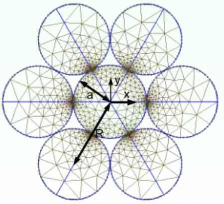
As an example, Fig. 6 shows the mesh of the cross-section of a strand with the following parameters: central wire with radius a and helical wires with helix radius R/a = 1.967 and angle Φ = 7.9◦. The cross-section of the central
cross-section of helical wires is no longer circular in the (eX, eY) plane. Note
that the helix radius R must be smaller than 2a, otherwise the adjacent helical wires would overlap each other. This example will be considered later in this section as well as in Part 2.
x y a
R
Figure 6: Mesh of seven-wire strand (R/a = 1.967, Φ = 7.9◦, a is the radius of the central
wire)
Now, the overall behavior of seven-wire strand is computed. The stiffness components studied are the axial stiffness and the coupling between extension and torsion, i.e. the 11 and 21 components of the matrix [khom] introduced
in (25). In order to compare results obtained from the 2D FE model with the reference solution of Ghoreishi et al. (2007), we set R/a = 2, ν = 0.3 and the stiffness components are written in the dimensionless form: k11 =
khom
11 /(EπR2), k21= k21hom/(EπR3).
Fig. 7 displays the variation of the axial stiffness k11 as a function of the
helix angle Φ, which varies between 2.5◦ and 35◦. For Φ ≤ 25◦, the difference
between the two results is below 2%. This difference increases with Φ and reaches 10% for Φ = 35◦.
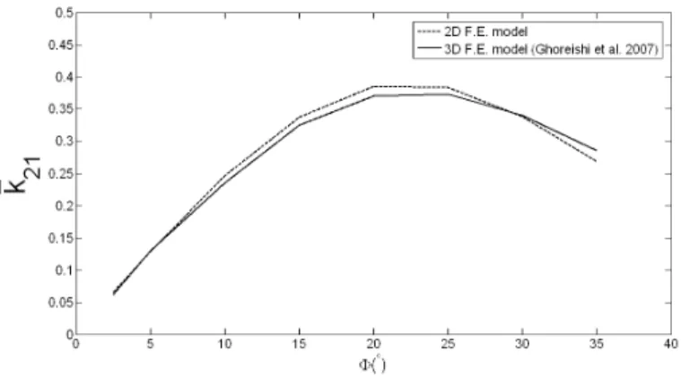
The variation of the coupling term k21 as a function of the helix angle Φ is
shown in Fig. 8. For Φ ≤ 8◦, the coupling term obtained by the two FE models
are very close. For large helix angle, the difference between the two solutions is below 4%.
Figure 7: Dimensionless axial stiffness of seven-wire strand. k11vs. Φ. R/a = 2.
Figure 8: Dimensionless stiffness coupling term of seven-wire strand. k21vs. Φ. R/a = 2.
The difference between the 2D and the reference 3D FE solutions can be explained by the use of a different mesh in the 2D model compared to the reference model. Indeed, the 2D mesh of a seven-wire strand with Φ = 5◦
reference 3D model is made of 72 elements and 210 nodes. Both the 2D and 3D FE models use quadratic elements. Moreover, an elliptical approximation of the cross-section shape was used in the 3D model, while the geometry is rigorously represented in the 2D model, according to Eq. (14). However as can be seen from Fig. (2), this approximation seems to be justified for examples studied with Φ ≤ 35◦
Overall the macroscopic behavior of the seven-wire strand computed by the 2D FE model according to the homogenization approach is in good agreement with that obtained from the 3D model. This provides a second validation of the helical computational homogenization approach.
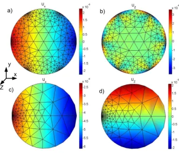
Lastly, microscopic displacements computed using the 2D FE model are an-alyzed. From the symmetry between the six helical wires, the displacements of only one peripheral wire is discussed. Fig. 9 shows the microscopic dis-placements in the cross-section of the seven-wire strand considered in Fig. 6 (R/a = 1.967, Φ = 7.9◦), subjected to EE = 0.6%. The in plane component
u2
x of the central and the peripheral wire are shown in Fig. 9(a) and (c),
re-spectively. One can observe the Poisson effect, with a linear evolution over the cross-section of u2
xin the central wire, and an affine evolution in the peripheral
wire, which is maintained in contact with the central wire. The axial displace-ment is presented in Fig. 9(b) and (d) for the central and the peripheral wire, respectively. One can notice that for the central wire the microscopic axial dis-placement is close to zero except in the vicinity of contact points where small variations occur. In the helical wire, a linear evolution of the microscopic axial displacement over the cross-section is found, due to local bending. For this ex-ample, the core wire radius is a = 2.7mm (the helical wire radius being 0.967a). Material properties are: ν = 0.28 and E = 2.17e11P a. The computed axial force and torque are T = 190.3kN and M = 118.1N.m. This example will used in Part 2 of this paper, for wave propagation analysis in prestressed strands.
a) b) c) x y Z d)
Figure 9: Dimensionless microscopic displacements of a seven-wire strand under axial defor-mation EE= 0.6%. (a) u2
x/a and (b) u2ζ/a in the central wire (c) u2x/a and (d) u2ζ/a in the
peripheral wire.
7. Conclusions
In this paper, the asymptotic expansion method has been applied to helical structures subjected to axial loads (traction and torsion) at its end sections. Thanks to the use of a twisted coordinate system, the 3D elastic problem has been reduced to a 2D microscopic problem posed on the cross-section and a 1D macroscopic beam problem, which has an analytical solution. Therefore the main contribution of this work is the derivation of the 2D microscopic problem, which fully exploits the translational invariance of the problem. The solution of this problem enables the computation of the overall beam stiffness as well as mi-croscopic stresses corresponding to a given mami-croscopic loading. The proposed approach has been validated for helical single wire structures and seven-wire strands and compares favorably with reference analytical results or 3D FE com-putations.
order to take into account effects of prestress and geometry deformation on wave propagation.
References
Ancker, C.J., Goodier, J.N., 1958. Pitch and curvature corrections for helical springs. Journal of Applied Mechanics , 466–470.
Argatov, I., 2011. Response of a wire rope strand to axial and torsional loads: Asymptotic modeling of the effect of interwire contact deformations. Inter-national Journal of Solids and Structures 48, 1413–1423.
Bajas, H., Durville, D., Ciazynski, D., Devred, A., 2010. Numerical simula-tion of the mechanical behavior of iter cable-in-conduit conductors. IEEE Transactions on Applied Superconductivity 20, 1467–1470.
Boso, D.P., Lefik, M., Schrefler, B.A., 2006. Homogenisation methods for the thermo-mechanical analysis of nb3sn strand. Cryogenics 46, 569–580.
Buannic, N., Cartraud, P., 2000. Higher-order asymptotic model for a het-erogeneous beam, including corrections due to end effects, in: Proc. of 41st AIAA/ASME/ASCE/AHS/ASC Structures, Structural Dynamics, and Ma-terials Conference.
Buannic, N., Cartraud, P., 2001a. Higher-order effective modelling of periodic heterogeneous beams - Part 1: Asymptotic expansion method. International Journal of Solids and Structures 38, 7139–7161.
Buannic, N., Cartraud, P., 2001b. Higher-order effective modelling of periodic heterogeneous beams - Part 2: Derivation of the proper boundary condi-tions for the interior asymptotic solution. International Journal of Solids and Structures 38, 7163–7180.
Cartraud, P., Messager, T., 2006. Computational homogenization of periodic beam-like structures. International Journal of Solids and Structures 43, 686– 696.
Chapelle, D., Bathe, K.J., 2003. The Finite Element Analysis of Shells-Fundamentals. Springer.
Costello, G.A., 1977. Theory of Wire Rope. Springer.
Durville, D., 1998. Mod´elisation du comportement m´ecanique de cˆables m´etalliques. Revue Europ´eenne des El´ements Finis 7, 9–22.
Erd¨onmez, C., ˙Imrak, C.E., 2011. New approaches for model generation and analysis for wire rope. in Computational Science and Its Applications - ICCSA 2011, Lecture Notes in Computer Science, B. Murgante, O. Gervasi, A. Igle-sias, D. Taniar, B. Apduhan editors, Springer , 103–111.
Ghoreishi, S.R., Messager, T., Cartraud, P., Davies, P., 2007. Validity and limitations of linear analytical models for steel wire strands under axial load-ing, using a 3d fe model. International Journal of Mechanical Sciences 49, 1251–1261.
Gnanavel, B., Parthasarathy, N., 2011. Effect of interfacial contact forces in radial contact wire strand. Archive of Applied Mechanics 81, 303–317.
Gray, A., Abbena, E., Salamon, S., 2006. Modern Differential Geometry of Curves and Surfaces with Mathmatica. 3rd Edition, Chapman and hall, Boca Raton.
˙Imrak, C.E., Erd¨onmez, C., 2010. On the problem of wire rope model generation with axial loading. Mathematical and Computational Applications 15, 259– 268.
Jiang, W.G., Henshall, J.L., 2000. A novel finite element model for helical springs. Finite Elements in Analysis and Design 35, 363–377.
Jiang, W.G., Warby, M.K., Henshall, J.L., 2008. Statically indeterminate con-tacts in axially loaded wire strand. European Journal of Mechanics A/Solids 27, 69–78.
Jiang, W.G., Yao, M.S., Walton, J.M., 1999. A concise finite element model for simple straight wire rope strand. International Journal of Mechanical Sciences 41, 143–161.
Jolicoeur, C., Cardou, A., 1991. A numerical comparison of current mathe-matical models of twisted wire cables under axisymmetric loads. Journal of Energy Resources Technology 113, 241–249.
Kalamkarov, A.L., Kolpakov, A.G., 1997. Analysis, Design and Optimization of Composite Structures. Wiley.
Kolpakov, A.G., 1991. Calculation of the characteristics of thin elastic rods with a periodic structure. J. Appl. Math. Mech. 55, 358–365.
Messager, T., Cartraud, P., 2008. Homogenization of helical beam-like struc-tures: application to single-walled carbon nanotubes. Computational Me-chanics 41, 335–346.
Nawrocki, A., Labrosse, M., 2000. A finite element model for simple straight wire rope strands. Computers and Structures 77, 345–359.
Nemov, A.S., Boso, D.P., Voynov, I.B., Borovkov, A.I., Schrefler, B.A., 2010. Generalized stiffness coefficients for iter superconducting cables, direct fe modeling and initial configuration. Cryogenics 50, 304–313.
Nicolet, A., Movchan, A.B., Geuzaine, C., Zolla, F., Guenneau, S., 2007. High order asymptotic analysis of twisted electrostatic problems. Physica B: Con-densed Matter 394, 335–338.
Nicolet, A., Zola, F., 2007. Finite element analysis of helicoidal waveguides. Measurement and Technology 28, 67–70.
Nicolet, A., Zola, F., Guenneau, S., 2004. Modeling of twisted optical waveg-uides with edge elements. The European Physical Journal Applied Physics 28, 153–157.
Onipede, O., Dong, S.B., 1996. Propagating waves and end modes in pretwisted beams. Journal of Sound and Vibration 195, 313–330.
P´aczelt, I., Beleznai, R., 2011. Nonlinear contact-theory for analysis of wire rope strand using high-order approximation in the fem. Computers and Structures 89, 1004–1025.
Sanchez-Hubert, J., Sanchez-Palencia, E., 1992. Introduction aux m´ethodes asymptotiques et l’homog´en´eisation. Masson, Paris.
Stanova, E., Fedorko, G., Fabian, M., Kmet, S., 2011a. Computer modelling of wire strands and ropes part i: Theory and computer implementation. Ad-vances in Engineering Software 42, 305–315.
Stanova, E., Fedorko, G., Fabian, M., Kmet, S., 2011b. Computer modelling of wire strands and ropes part ii: Finite element-based applications. Advances in Engineering Software 42, 322–331.
Synge, J.L., Schild, A., 1978. Tensor Calculus. Dover.
Trabucho, L., Via˜no, J.M., 1996. Mathematical modelling of rods. Handbook of Numerical Analysis IV, P.G. Ciarlet, J.L. Lions editors, North-Holland , 487–974.
Treyss`ede, F., 2008. Elastic waves in helical waveguides. Wave Motion 45, 457–470.
Treyss`ede, F., 2011. Mode propagation in curved waveguides and scattering by inhomogeneities: application to the elastodynamics of helical structures. Journal of the Acoustical Society of America 129, 1857–1868.
Treyss`ede, F., Laguerre, L., 2010. Investigation of elastic modes propagating in multi-wire helical waveguides. Journal of Sound and Vibration 329, 1702– 1716.
Wahl, A.M., 1963. Mechanical Springs. Second Edition, Mc Graw-Hill, Inc., New York.
Wempner, G., 1981. Mechanics of Solids with Applications to Thin Bodies. Sijthoff and Noordhoff, The Netherlands.