A Compact Spherical RGBD Keyframe-based Representation

HAL Id: hal-01121089

https://hal.inria.fr/hal-01121089

Submitted on 27 Feb 2015

HAL is a multi-disciplinary open access

archive for the deposit and dissemination of

sci-entific research documents, whether they are

pub-lished or not. The documents may come from

teaching and research institutions in France or

abroad, or from public or private research centers.

L’archive ouverte pluridisciplinaire HAL, est

destinée au dépôt et à la diffusion de documents

scientifiques de niveau recherche, publiés ou non,

émanant des établissements d’enseignement et de

recherche français ou étrangers, des laboratoires

publics ou privés.

A Compact Spherical RGBD Keyframe-based

Representation

Tawsif Gokhool, Renato Martins, Patrick Rives, Noëla Despré

To cite this version:

Tawsif Gokhool, Renato Martins, Patrick Rives, Noëla Despré.

A Compact Spherical RGBD

Keyframe-based Representation. IEEE Int. Conf. on Robotics and Automation, ICRA’15, May

2015, Seattle, United States. �hal-01121089�

A Compact Spherical RGBD Keyframe-based Representation

Tawsif Gokhool, Renato Martins, Patrick Rives and No¨ela Despr´e

Abstract— This paper proposes an environmental

represen-tation approach based on hybrid metric and topological maps as a key component for mobile robot navigation. Focus is made on an ego-centric pose graph structure by the use of Keyframes to capture the local properties of the scene. With the aim of reducing data redundancy, suppress sensor noise whilst maintaining a dense compact representation of the environment, neighbouring augmented spheres are fused in a single representation. To this end, an uncertainty error model propagation is formulated for outlier rejection and data fusion, enhanced with the notion of landmark stability over time. Finally, our algorithm is tested thoroughly on a newly developed wide angle3600 field of view (FOV) spherical sensor where improvements such as trajectory drift, compactness and reduced tracking error are demonstrated.

I. INTRODUCTION

Visual mapping is a required capability for autonomous robots and a key component for long term navigation and localisation. Inherent limitations of GPS in terms of dropping accuracy in densely populated urban environments or lack of observability in indoor settings have propelled the ap-plications of visual mapping techniques. Moreover, the rich content provided by vision sensors maximises the description of the environment.

A metric map emerges from a locally defined reference frame and all information acquired along the trajectory is then represented in relation to this reference frame. Hence, localisation in a metric map is represented by a pose ob-tained from frame to frame odometry. The benefit of this approach is its precision at the local level allowing precise navigation. On the other hand, this representation is prone to drift phenomena which becomes significant over extended trajectories. Furthermore, the amount of information that is accumulated introduces considerable problems in memory management due to limited capacity.

By contrast, a topological map provides a good trade-off solution to the above-mentioned issues. Distinct places of the environment are defined by nodes and joined together by edges representing the accessibility between places generat-ing a graph. This representation not only brgenerat-ings about a good abstraction level of the environment but common tasks such as homing, navigation, exploration and path planning become more efficient. However, the lack of metric information may render some of these tasks precision deficient as only rough

*This work is funded by EADS/Airbus under contract number N.7128 and by CNPq of Brazil under contract number 216026/2013-0

T. Gokhool, R. Martins and P. Rives are with INRIA Sophia-Antipolis, France {tawsif.gokhool, renato-jose.martins, patrick.rives}@inria.fr

No¨ela Despr´e is with Airbus Defence and Space, Toulouse, France

noela.despre@astrium.eads.net

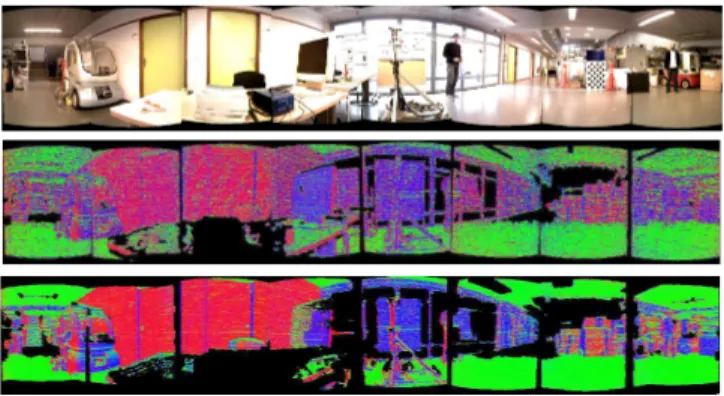
Fig. 1. Normal consistency between raw and improved spherical keyframe model of one of the nodes of the skeletal pose graph. The colours in the figure encode surface normal orientations, where better consistence is achieved when local planar regions depicts the same colour

estimates are available. Eventually, to maximise the benefits of these two complementary approaches, it is needed to strike the right balance between metric and topological maps which leads us to the term topo-metric maps as in [1].

In this context, accurate and compact 3D environment modelling and reconstruction has drawn increased interests within the vision and robotics community over the years as it is perceived as a vital tool for Visual SLAM techniques in realising tasks such as localisation, navigation, exploration and path planning [3]. Planar representation of the envi-ronment achieve fast localisation [6], but they ignore other useful information in the scene. Space discretisation using volumetric methods such as signed distance functions [17], with combined sparse representations using octrees [18], though they have received widespread attention recently due to their reconstruction quality do however present certain caveats. Storage capacity and computational burden restrict their application to limited scales. To provide alternatives, a different approach consisting of multi-view rendering was proposed in [15]. Depth maps captured in a window of n views are rendered in a central view taken as the reference frame and are fused based on a stability analysis of the projected measurements. On a similar note, recent works undertaken in [12] adopted a multi-keyframe fusion approach by forward warping and blending to create a novel synthe-sized depth map.

When exploring vast scale environments, many frames sharing redundant information clutter the memory space considerably. Furthermore, performing frame to frame regis-tration introduces drift in the trajectory due to uncertainty in the estimated pose as pointed out in [9]. The idea to retain keyframes based on predefined criteria proves very useful within a sparse skeletal pose graph, which is the chosen

model for our compact environment representation. II. METHODOLOGY ANDCONTRIBUTIONS

Our aim is concentrated around building ego-centric topo-metric maps represented as a graph of keyframes, spread by spherical RGBD nodes. A locally defined geo-referenced frame is taken as an initial model which is then refined over the course of the trajectory by neighbouring frames’ render-ing. This not only reduces data redundancy but also help in suppressing sensor noise whilst contributing significantly in drift reduction. A generic uncertainty propagation model is devised and leaned upon a data association framework for discrepancy detection between the measured and observed data. We build upon the above two concepts to introduce the notion of landmark stability over time. This is an important aspect for intelligent 3D points selection which serve as better potential candidates for subsequent inter frame to keyframe motion estimation task.

This work is directly related to two previous syntheses of [4] and [12]. The former differs from our approach in the sense that it is a sparse feature based technique and only consider depth information propagation. On the other hand, the latter aboard a similar dense based method to ours but without considering error models and a simpler Mahalanobis test defines the hypothesis for outlier rejection. Additionally, we build on a previous work of [13] which constitutes of building a saliency map for each reference model, by adding the concept of stability of the underlying 3D structure.

Key contributions of this work are outlined as follows:

• development of a generic spherical uncertainty error propagation model, which can be easily adapted to other sensor models (e.g. perspective RGBD cameras)

• a coherent dense outlier rejection and data fusion

framework relying on the proposed uncertainty model, yielding more precise spherical keyframes

• dynamic 3D points are tracked along the trajectory and

are pruned out by skimming down a saliency map The rest of this paper is organised as follows: basic concepts are first introduced and shall serve as the backbone to allow a smooth transition between respective sections. Then the uncertainty error model is presented followed by the fusion stage. Subsequently, the problem of dynamic 3D points is tackled leading to a direct application of the saliency map. An experimental and results section verifies all of the above derived concepts before wrapping up with a final conclusion and some perspectives for future work.

III. PRELIMINARIES

An augmented spherical image _{S = {I, D} is composed} of_{I ∈ [0, 1]}m×n as pixel intensities and_{D ∈ R}m×n as the depth information for each pixel in_{I. The basic environment} representation consists of a set of spheres acquired over time together with a set of rigid transforms T _{∈ SE(3)} connecting adjacent spheres (e.g. Tij liesSj andSi) – this

representation is well described in [14].

The spherical images are encoded in a 2D image and the mapping between the image pixel coordinates p and depth to

cartesian coordinates is given by g : (u, v, 1)7→ q, g(p) = ρqS(p), with qS being the point representation in the unit

spherical space S2

andρ =D(p) is radial depth. The inverse transformg−1_{corresponds to the spherical projection model.}

Point coordinates correspondences between spheres are given by the warping functionw, under observability condi-tions at different viewpoints. Given a pixel coordinate p∗, its coordinate p in another sphere related by a rigid transform T is given by a screw transform from the 3D q = g(p∗₎

followed by a spherical projection:

p= w(p∗_{, T) = g}−1 „ [I 0]T−1 » g(p∗₎ 1 –« , (1)

where I is a(3_{× 3) identity matrix and 0 is a (3 × 1) zeros} vector. In the following, spherical RGBD registration and keyframe based environment representations are introduced. A. Spherical Registration and Keyframe Selection

The relative location between raw spheres is obtained using a visual spherical registration procedure [12] [7]. Given a first pose estimate bTof T= bTT(x), the sphere to sphere registration problem consists of incrementally estimating a 6 degrees of freedom (DOF) pose x _{∈ R}6

, through the minimization of a robust hybrid photometric and geometric error cost function FS =

1 2keIk 2 I+λ 2 2keρk 2 D, which can be

written explicitly as:

FS=1₂P_p∗W I_(p∗₎‚‚_‚I“_w(p∗_{, bTT(x))}”_{− I}∗`_p∗´‚‚_‚2₊ λ2 2 P p∗W D_(p∗₎‚‚ ‚nT “ g(w(p∗_{, bTT(x))) − bTT(x)g}∗_(p∗₎”‚‚ ‚ 2 (2)

wherew(•) is the warping function as in (1), λ is a tuning parameter to effectively balance the two cost functions, WI _{and W}D _{are weights relating the confidence of each}

measure and n is the normal computed from the cross product of adjacent points from q(p∗_{). The linearization}

of the over-determined system of equations (2) leads to a classic iterative Least Mean Squares (ILMS) solution. Furthermore for computational efficiency, one can choose a subset of more informative pixels (salient points) that yield enough constraints over the 6DOF, without compromising the accuracy of the pose estimate.

This simple registration procedure applied for each se-quential pair of spheres allows to represent the scene struc-ture, but subjected to cumulative VO errors and scalability issues due to long-term frame accumulation. The idea to retain just some spherical keyframes, based on predefined criteria, proves very useful to overcome these issues and generate a more compact graph scene representation. A criteria based on differential entropy approach [9] has been applied in this work for keyframe selection.

IV. SPHERICALUNCERTAINTYPROPAGATION AND

MODELFUSION

Our approach to topometric map building is an egocentric representation operating locally on sensor data. The con-cept of proximity used to combine information is evaluated

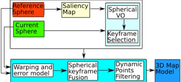
Reference Sphere Current Sphere Saliency Map Spherical VO Keyframe Selection Dynamic Points Filtering 3D Map Model Spherical keyframe Fusion Warping and error model

Fig. 2. Full system pipeline

mainly with the entropy similarity criteria after the regis-tration procedure. Instead of performing a complete bundle adjustment along all parameters including poses and structure for the full set of close raw spheres_Sito the related keyframe

model_S∗_{, the procedure is done incrementally in two stages.}

The concept is as follows: primarily, given a reference sphere _S∗ and a candidate sphere _{S, the cost function in} (2) is employed to extract T= bTT(x) and the entropy criteria is applied for a similarity measure between the tuple {S∗_,

S}. While this metric is below a predefined threshold, the keyframe model is refined in a second stage – warping S and carrying out a geometric and photometric fusion procedure is composed of three steps:

• warpingS and its resulting model error propagation • data fusion with occlusions and outlier rejection

• wise 3D point selection based on stable salient points which are detailed in the following subsections. The full system pipeline is depicted in figure (2).

A. Warped Sphere Uncertainty

Warping the augmented sphere _{S generates a synthetic} view of the scene _Sw = {Iw,Dw}, as it would appear

from a new viewpoint. This section aims to represent the confidence of the elements in Sw, which clearly depends

on the combination of an apriori pixel position, the depth and the pose errors over a set of geometric and projective operations – the warping function as in (1). Starting with Dw, the projected depth image is

Dw(p∗) = Dt(w(p∗, T)) and Dt(p) = p qw(p, T)⊤qw(p, T) with qw(p, T) = „ [I 0]T » g(p) 1 –« (3)

The uncertainty of the final warped depthσ2

Dw then depends on two terms Σw and σ2Dt; the former relates to the error due to the warpingw of pixel correspondences between two spheres and the latter, to the depth image representation in the reference coordinate systemσ2

Dt.

Before introducing these two terms, let’s represent the uncertainty due to the combination of pose T and a cartesian 3D point q errors. Taking a first order approximation of q= g(p) = ρqS, the error can be decomposed as:

Σq(p) = σρ2qSq⊤S+ ρ2ΣqS =

σ2ρ

ρ2g(p)g(p) ⊤_{+ ρ}2_Σ

g(p)/ρ (4)

The basic error model for the raw depth is proportional to its fourth degree itself: σ2

ρ∝ ρ 4

, which can be applied

to both stereopsis and active depth measurement systems (for instance see [10] for details). The next step consists of combining the uncertain rigid transform T with the errors in q. Given the mean of the 6DOF ¯x={tx, ty, tz, θ, φ, ψ}

in 3D+YPR form and its covariance Σx, for qw(p, T) =

Rq+ t = Rg(p) + t ,

Σqw(p, T) = Jq(q, ¯x)ΣqJq(q, ¯x)⊤+ JT(q, ¯x)ΣxJT(q, ¯x)⊤ = RΣqR⊤+ MΣxM⊤,

(5)

withΣq as in (4) and the general formula of M is given in

[2]. The first termΣwusing (5) and (1) is given by:

Σw(p∗, T) = Jg−1(qw(•))Σqw(•)Jg−1(qw(•))⊤ (6)

where Jg−1 is the jacobian of the spherical projection (the inverse of g) and (•) = (p∗_{, T}−1_{). The second term}

expression for the depth represented in the coordinate system of the reference sphere using the warped 3D point in (5) and (3) is straightforward σ2_Dt(p ∗_{, T) = J} Dt(qw(p ∗_{, T))Σ} qw(p ∗_{, T)J} Dt(qw(p ∗_{, T))}⊤ (7) withJDt(z) = (z ⊤_/√_z⊤_z).

The uncertainty indexσ2

Dw is then the normalized covari-ance given by:

σ2 Dw(p) = σ 2 Dt(p)/(qw(p, T) ⊤_q w(p, T)) 2 (8) Finally, under the assumption of Lambertian surfaces, the photometric component is simply _Iw(p∗) = I(w(p∗, T))

and it’s uncertaintyσ2

I is set by a robust weighting function

on the error using a Huber’s M-estimator as in [14]. B. Spherical Keyframe Fusion

Before combining the keyframe reference model_S∗ with that of the transformed observation_Sw, a probabilistic test is

performed to exclude outlier pixel measurements from_Sw,

allowing fusion to occur only if the raw observation agrees with its corresponding value in_S∗_.

Hence, the tuple A = {D∗_,

Dw} and B = {I∗,Iw}

are defined as the sets of model predicted and measured depth and intensity values respectively. Finally, let a class c: _D∗_{(p) =}

Dw(p) relate to the case where the

measure-ment value agrees with its corresponding observation value. Inspired by the work of [16], the Bayesian framework for data association leads us to:

p(c|A, B) =p(A,B|c)p(c)

p(A,B) (9)

Applying independence rule between depth and visual prop-erties and assuming a uniform prior on the classc (can also be learned from supervised techniques), the above expression simplifies to:

p(c|A, B) ∝ p(A|c)p(B|c) (10)

Treating each term independently, the first term of equation (10) is devised as p(A_{|c) = p(D}w(p)|D∗(p), c), whereby

marginalizing over the true depth valueρi leads to:

p(Dw(p)|D∗(p), c) = Z

p(Dw(p)|ρi,D∗(p), c)p(ρi|D∗(p), c)dρi (11)

Approximating both probability density functions as Gaussians, the above integral reduces to: p(A|c) =

N (Dw(p)|D∗(p), σDw(p), σD∗(p)). Following a similar treatment,p(B_{|c) = N (Iw}(p)|I∗_{(p), σ}

Iw(p), σI∗(p)). Since equation (10) can be viewed as a likelihood function, it is easier to analytically work with its logarithm in order to extract a decision boundary. Pluggingp(A_{|c) and p(}B_{|c) into}

(10) and taking its negative log gives the following decision rule for an inlier observation value:

(Dw(p) − D∗(p))2 σ2 Dw(p) + σ 2 D∗(p) +(Iw(p) − I ∗_(p))2 σ2 Iw(p) + σ 2 I∗(p) < λ2M, (12)

relating to the square of the Mahalanobis distance. The thresholdλ2

M is obtained by looking up theχ 2 2 table.

Ultimately, we close up with a classic fusion stage, whereby depth and appearance based consistencies are co-alesced to obtain an improved estimate of the keyframe sphere. Warped values that pass the test in (12) are fused up by combining their respective uncertainties as follows:

I∗ k+1(p) = WIk(p)Ik∗(p) + ΠI(p)Iw(p) WI k(p) + ΠI(p) , D∗ k+1(p) = WD_k(p)D∗ k(p) + ΠD(p)Dw(p) WD k(p) + ΠD(p) (13)

for the intensity and depth values respectively and weight update:

WIk+1= WIk+ ΠI and WDk+1= WkD+ ΠD (14)

where ΠI(p) = 1/σ2Iw(p) and ΠD(p) = 1/σ

2

Dw(p) from the uncertainty warp propagation in sec. IV-A.

C. Dynamic 3D points filtering

So far, the problem of data fusion of consistent estimates in a local model has been addressed. But to improve the performance of any model, another important aspect of any mapping system is to limit if not completely eliminate the negative effects of dynamic points. These points exhibit erratic behaviours along the trajectory and as a matter of fact, they are highly unstable. There are however different levels of “dynamicity” as mentioned in [11]. Points/landmarks observed can exhibit a gradual degradation over time, while others may undergo a sudden brutal change – the case of an occlusion for example. The latter being considerably apparent in indoor environments where small viewpoint changes can trigger a large part of a scene to be occluded. Other cases are observations undergoing cyclic dynamics (doors opening and closing). Whilst the above-mentioned behaviours are learned in clusters [11], in this work, points with periodic dynamics are simply evaluated as occlusion phenomena.

The probabilistic framework for data association devel-oped in the section IV-B is a perfect fit to filter out in-consistent data. 3D points giving a positive response to test equation (12) are given a vote1, or otherwise attributed a 0. This gives rise to a confidence map_C∗

i(k) which is updated as follows: C∗ i(k + 1) = ( C∗ i(k) + 1, if λ(95%)M <5.991 0, otherwise (15)

Algorithm 1 3D Points Pruning using Saliency map

Require: ˘S∗

sal,Ci∗(k), N, n ¯ return Optimal Set A10%∈ S∗sal Initialise new A

for i=S∗

sal(p∗) = 1 to S∗sal(p∗) = max do compute p(occur)(p∗i) compute γk+1(p∗i) compute p(stable)(p∗i) if p(stable)(p∗i) ≥ 0.8 then A[ i ] ←− p∗ i end if if length(A[ i ]) ≥ A10%then break end if end for

Hence, the probability of occurence is given by:

p(occur) =C ∗ i(k + N )

N , (16)

wheren is the total number of accumulated views between two consecutive keyframes. p(occur), though it gives an indication on how many times a point has been tracked along the trajectory, it can however not distinguish between noisy data or an occlusion. Treading on a similar technique to that adopted in [8], a Markov observation independence is imposed. In the event that a landmark/3D point has been detected at time instantk, it is most probable to appear again atk + 1 irrespective of its past history. On the contrary, if it has not been re-observed, this may mean that the landmark is quite noisy/unstable or has been removed indeterminately from the environment and has little chance to appear again. These hypotheses are formally translated as follows:

γk+1(p∗) = (

1, if p∗k= 1

(1 − p(occur))n_{, otherwise} (17)

Finally, the overall stability of the point is given as:

p(stable) = γk+1p(occur) (18)

D. Application to Saliency map

Instead of naively dropping out points below a certain threshold, for e.g, p(stable) < 0.8, they are better pruned out of a saliency map [13]. A saliency map, S∗

sal, is the

outcome of careful selection of the most informative points, best representing a 6 degree of freedom pose, x _{∈ R}6

, based on a Normal Flow Constraint spherical jacobian. The underlying algorithm is outlined in algorithm (1). The green and red sub-blocks in figure (3) represent the set of inliers

b TT(x) `_{( b} TT(x)´−1 set B set A A ∩ Bw _{A − A10% ∩ B}w A10%

and outliers respectively, while the yellow one corresponds to the set of pixels which belong to the universal set{U : U = A_{∪ B}w_{} but which have not been pruned out. This happens} when the Keyframe criteria based on an entropy ratioα [7][9] is reached. The latter is an abstraction of uncertainty related to the pose x along the trajectory, whose behaviour shall be discussed in the results section.

The novelty of this approach compared to the initial work of [13] is two-fold. Firstly, the notion of uncertainty is incorporated in spherical pixel tracking. Secondly, as new incoming frames are acquired, rasterised and fused, the information content of the initial model is enriched and hence the saliency map needs updating. This gives a newly ordered set of pixels to which is attributed a corresponding stability factor. Based on this information, an enhanced pixel selection is performed consisting of pixels with a greater chance of occurence in the subsequent frame. This set of pixel shall then be used for the forthcoming frame to keyframe motion estimation task. Eventually, between an updated model at timet0and the following re-initialised one, att_n, an optimal

mix of information sharing happens between the two. V. EXPERIMENTS ANDRESULTS

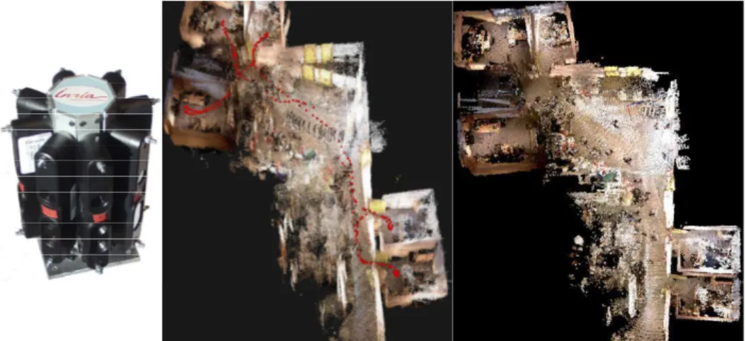
A new sensor for a large field of view RGBD image acquisition has been used in this work. This device integrates 8 Asus Xtion Pro Live (Asus XPL) sensors as shown in figure (4)(left) and allows to build a spherical representation. The chosen configuration offers the advantage of creating full 360◦_{RGBD images of the scene isometrically, i.e. the same}

solid angle is assigned to each pixel. This permits to apply directly some operations, like point cloud reconstruction, photo consistency alignment or image subsampling. For more information about sensor calibration and spherical RGBD construction, the interested reader is referred to [5].

Our experimental test bench consists of the spherical sen-sor embarked on a mobile experimental platform and driven around in an indoor office building environment for a first learning phase whilst spherical RGBD data is acquired online and registered in a database. In this work, we do not address the problem of the real time aspect of autonomous navigation and mapping but rather investigate ways of building robust and compact environment representations by capturing the observability and dynamics of the latter. Along this stream-line, reliable estimates coming from sensor data based on 3D geometrical structure are combined together to serve as a useful purpose for later navigation and localisation tasks which can thereafter be treated with better precision online. Our algorithm has been extensively tested on a dataset1_of

around 2500 frames covering a total distance of around60m. Figures 5(a), (b) illustrates the trajectories obtained from two experimented methods, namely; RGBD registration without (method 1) and with (method 2) keyframe fusion in order to identify the added value of the fusion stage. The visible discrepancy between the trajectories for the same pathway

1_{video url:(http://www-sop.inria.fr/members/Tawsif.Gokhool/icra15.html)}

highlights the effects of erroneous pose estimation that oc-curs along the trajectories. This is even more emphasized by inspecting the 3D structure of the reconstructed environment as shown by figures (4)(centre), (4)(right) where the two images correspond to the sequence with and without fusion; method 1 and method 2 respectively. In detail, reconstruc-tion with method 1 demonstrates the effects of duplicated structures (especially surrounding wall structures) which is explained by the fact that point clouds are not perfectly stitched together on revisited areas due to inherent presence of rotational drift, that is more pronounced than translational drift. However, these effects are well reduced by the fusion stage though not completely eliminated as illustrated in figure 4(right). The red dots on the reconstruction images are attributed to the reference spheres initialised along the trajectories using the keyframe criteria described in section III-A. 270 key spheres were recorded for method 1 while only 67 were registered for method 2.

Finally, comparing figures 5(a), (b), the gain in compact-ness for method 2 is clearly demonstrated by the sparse positioning of keyframes in the skeletal pose graph structure. Figure 5(c) depicts the behaviour of our keyframe selection entropy-based criteria α . The threshold for α is generally heuristically tuned. For method 1, a preset value of 0.96 was used based on the number of iterations to convergence of the cost function outlined in section III-A. With the fusion stage, the value ofα was allowed to drop to 0.78 with generally faster convergence achieved. Figure 5(d) confirms the motion estimation quality of method 2 as it exhibits a lower error norm across frames as compared to method 1. Figure (1) depicts the quality of the depth map before and after applying the filtering technique. The colours in the figure represent normal orientations with respect to the underlying surfaces.

VI. CONCLUSION

In this work, a framework for hybrid metric and topo-logical maps in a single compact skeletal pose graph rep-resentation has been proposed. Two methods have been experimented and the importance of data fusion has been highlighted with the benefits of reducing data noise, re-dundancy, tracking drift as well as maintaining a compact environment representation using keyframes.

Our activities are centered around building robust and sta-ble environment representations for lifelong navigation and map building. Future investigations will be directed towards gathering more semantic information about the environment to be able to further exploit the quality and stability of the encompassing 3D structure.

ACKNOWLEDGMENT

The authors extend their warmest gratitude to Maxime Meilland and Panagiotis Papadakis for their critical insights and suggestions in improving the material of this paper.

REFERENCES

[1] H. Badino, D. Huber, and T. Kanade. Visual Topometric Localization. In Intelligent Vehicles Symposium, Baden-Baden, Germany, June 2011.

Fig. 4. Left:Multi RGBD acquisition system, centre and right:Reconstruction quality comparison (bird-eye view) -8 -4 0 4 -4 0 4 8 12 Z /m X /m (a) Trajectory Plot

-8 -4 0 4 -4 0 4 8 12 Z /m X /m (b) Trajectory Plot 0.75 0.8 0.85 0.9 0.95 1 0 4 8 12 α Distance/m (c) Entropy ratio vs Distance Travelled/m.

0 0.5 1 1.5 2 0 40 80 120 160 k e k N × 1 0 − 3 Frame Nos. (d) Error norm vs Frame Nos.

method 1 Ref method 1

method 2 Ref method 2

Fig. 5. Performance comparison between method 1: RGBD spherical registration without keyframe fusion and method 2 : RGBD spherical registration with fusion. (plots in red and blue refer to methods 1 and 2 respectively)

[2] J-L. Blanco. A tutorial on se(3) transformation parameterizations and on-manifold optimization. Technical report, Univ. of Malaga, 2010. [3] E. Bylow, J. Sturm, C. Kerl, and F. Kahl. Real- Time camera tracking

and 3D Reconstruction using signed distance functions. In RSS, 2013. [4] I. Dryanovski, R. Valenti, and J. Xiao. Fast visual odometry and

mapping from rgb-d data. In ICRA, 2013.

[5] E. Fern´andez-Moral, J. Gonz´alez-Jim´enez, P. Rives, and V. Ar´evalo. Extrinsic calibration of a set of range cameras in 5 seconds without pattern. In IROS. IEEE/RSJ, sep 2014.

[6] E. Fern´andez-Moral, W. Mayol-Cuevas, V. Ar´evalo, and J. Gonz´alez-Jim´enez. Fast place recognition with plane-based maps. In ICRA, 2013.

[7] T. Gokhool, M. Meilland, P. Rives, and E. Fern´andez-Moral. A Dense Map Building Approach from Spherical RGBD Images. In VISAPP, 2014.

[8] E. Johns and G-Z. Yang. Generative Methods for Long-Term Place Recognition in Dynamic Scenes. IJCV, 106(3), 2014.

[9] C. Kerl, J. Sturm, and D. Cremers. Dense Visual SLAM for RGB-D Cameras. In IROS, 2013.

[10] K. Khoshelham and S. Elberink. Accuracy and resolution of kinect depth data for indoor mapping applications. Sensors, 12(2), 2012.

[11] K. Konolige and J. Bowman. Towards lifelong Visual Maps. In IROS, 2009.

[12] M. Meilland and A. Comport. On unifying keyframe and voxel based dense visual SLAM at large scales. In IROS, 2013.

[13] M. Meilland, A. Comport, and P. Rives. A spherical robot-centered representation for urban navigation. In IROS, 2010.

[14] M. Meilland, A. Comport, and P. Rives. Dense visual mapping of large scale environments for real-time localisation. In IROS, 2011. [15] P. Merrell, A. Akbarzadeh, L. Wang, P. Mordohai, J-M. Frahm,

R. Yand, D. Nister, and M. Pollefeys. Real-Time Visibility-Based Fusion of Depth Maps. In ICCV, 2007.

[16] A. Murarka, J. Modayil, and B. Kuipers. Building Local Safety Maps for a Wheelchair Robot using Vision Lasers. In CRV, 2006. [17] R. Newcombe, S. Izadi, O. Hilliges, D. Molyneaux, D. Kim, A.

Davi-son, P. Kohli, J. Shotton, S. Hodges, and A. Fitzgibbon. KinectFusion: Real-Time Dense Surface Mapping and Tracking. In ISMAR, 2011. [18] F. Steinbr¨ucker, C. Kerl, J. Sturm, and D. Cremers. Large-scale

Multi-Resolution Surface Reconstruction from RGB-D Sequences . In ICCV, 2013.