HAL Id: hal-01087858
https://hal.inria.fr/hal-01087858
Submitted on 26 Nov 2014
HAL is a multi-disciplinary open access
archive for the deposit and dissemination of
sci-entific research documents, whether they are
pub-lished or not. The documents may come from
teaching and research institutions in France or
abroad, or from public or private research centers.
L’archive ouverte pluridisciplinaire HAL, est
destinée au dépôt et à la diffusion de documents
scientifiques de niveau recherche, publiés ou non,
émanant des établissements d’enseignement et de
recherche français ou étrangers, des laboratoires
publics ou privés.
Statistical Abstraction Boosts Design and Test
Efficiency of Evolving Critical Systems
Axel Legay, Sean Sedwards
To cite this version:
Axel Legay, Sean Sedwards. Statistical Abstraction Boosts Design and Test Efficiency of Evolving
Critical Systems. Leveraging Applications of Formal Methods, Verification and Validation.
Technolo-gies for Mastering Change, EasyConference, Oct 2014, Corfu, Greece. pp.4 - 25,
�10.1007/978-3-662-45234-9_2�. �hal-01087858�
Statistical Abstraction Boosts Design and Test
Efficiency of Evolving Critical Systems
Axel Legay and Sean Sedwards
Inria Rennes – Bretagne Atlantique
Abstract Monte Carlo simulations may be used to efficiently estimate critical properties of complex evolving systems but are nevertheless com-putationally intensive. Hence, when only part of a system is new or mod-ified it seems wasteful to re-simulate the parts that have not changed. It also seems unnecessary to perform many simulations of parts of a system whose behaviour does not vary significantly.
To increase the efficiency of designing and testing complex evolving sys-tems we present simulation techniques to allow such a system to be verified against behaviour-preserving statistical abstractions of its envi-ronment. We propose a frequency domain metric to judge the a priori performance of an abstraction and provide an a posteriori indicator to aid construction of abstractions optimised for critical properties.
1
Introduction
The low cost of hardware and demand for increased functionality make mod-ern computational systems highly complex. At the same time, such systems are designed to be extensible and adaptable, to account for new functionality, in-creased use and new technology. It is usually cost-efficient to allow a system to evolve piece-wise, rather than replace it entirely, such that over time it may not respect its original specification. A key challenge is therefore to ensure that the critical performance of evolving systems is maintained up to the point of their obsolescence.
The basic challenge has been addressed by robust tools and techniques de-veloped in the field of software engineering, which allow designers to specify and verify the performance of complex systems in terms of data flow. The level of abstraction of these techniques often does not include the precise dynamical be-haviour of the implementation, which may critically affect performance. Hence, to guarantee that the implementation of a system respects its specification it is necessary to consider detailed dynamical models. In particular, it is necessary to consider dynamics that specifically model the uncertainty encountered in real deployment.
1.1 Our Approach
To address the problem of designing and testing evolving critical systems [16] we focus on efficient ways to construct and formally verify large dynamical models
whose structure evolves over time. In particular, we consider systems comprising components whose dynamics may be represented by continuous time Markov chains (CTMC). CTMCs model uncertainty by probabilistic distributions and may also include deterministic behaviour (i.e., that happens with probability 1 in a given state). Importantly, CTMCs allow the verification and quantification of properties that include real time.
We consider verification of dynamical properties using model checking, where properties are specified in temporal logic [6]. Importantly, such logics typically in-clude an until operator, which expresses properties that inin-clude temporal causal-ity. To quantify uncertainty and to consider events in real time, numerical model checking extends this idea to probabilistic systems, such as modelled by CTMCs. Current numerical model checking algorithms are polynomial in the size of the state space [1,6], but the state space scales exponentially with respect to the number of interacting variables, i.e., the intuitive notion of the size of the sys-tem. Techniques such as symbolic model checking [5], partial order reduction [14], bounded model checking [3] and abstraction refinement [7] have made model checking much more efficient in certain cases, but the majority of real systems remain intractable.
Statistical model checking (SMC) is a Monte Carlo technique that avoids the ‘state explosion problem’ [6] of numerical model checking by estimating the probability of a property from the proportion of simulation traces that individ-ually satisfy it. SMC is largely immune to the size of the state space and takes advantage of Bernoulli random variable theory to provide confidence bounds for its estimates [20,25]. Since SMC requires independent simulation runs, verifi-cation can be efficiently divided on parallel computing architectures. SMC can thus offer a tractable approximate solution to industrial-scale numerical model checking problems that arise during design or certification of a system. SMC may nevertheless be computationally expensive with rare properties (which are often critical) and when high precision is required.
SMC relies on simulation, so in this work we propose a technique of statisti-cal abstraction to boost the efficiency of simulation. We show how to construct adequate statistical abstractions of external systems and we provide a corre-sponding stochastic simulation algorithm that maintains existing optimisations and respects the causality of the original system. We demonstrate that it is pos-sible to make useful gains in performance with suitable systems. We provide a metric to judge a priori that an abstraction is good and an indicator to warn when the abstraction is not good in practice. Importantly, we show that a statis-tical abstraction may be optimised for cristatis-tical rare properties, such that overall performance is better than simulation without abstraction.
The basic assumption of our approach is that we wish to apply SMC to a system comprising a core system in an environment of non-trivial external sys-tems. In particular, we assume that properties of the external systems are not of interest, but that the environment nevertheless influences and provides input to the core. In this context, we define an external system to be one whose behaviour is not affected by the behaviour of the core or other external systems. This may
seem like a severe restriction, but this topology occurs frequently because it is an efficient and reliable way to construct large systems from modules. A sim-ple examsim-ple is a network of sensing devices feeding a central controller. Our case study is a complex biological signalling network that has this topology. To consider more general interactions would eliminate the modularity that makes statistical abstraction feasible.
Our idea is to replace the external systems with simple characterisations of their output, i.e., of the input to the core system. To guarantee the correct time-dependent behaviour of the environment, we find the best approach is to construct an abstraction based on an empirical distribution of traces, created by independent simulations of the external systems. During subsequent investi-gation, the core system is simulated against traces chosen uniformly at random from the empirical distributions of each of the external systems. The abstrac-tions are constructed according to a metric based on frequency domain analysis. We make gains in performance because (i ) the external systems are simulated in the absence of other parts of the system, (ii ) the empirical distributions contain only the transitions of the variables that affect the core and (iii ) the empirical distributions contain the minimum number of traces to adequately represent the observed behaviour of the variables of interest.
SMC generally has very low memory requirements, so it is possible to take advantage of the unused memory to store distributions of pre-simulated traces. Such distributions can be memory intensive, so we also consider memory-efficient abstractions using Gaussian processes, to approximates the external system on the fly. We give results that demonstrate the potential of this approach, using frequency domain analysis to show that it is possible to construct abstractions that are statistically indistinguishable from empirical abstractions.
Although our idea is simple in concept, we must show that we can achieve a gain in performance and that our algorithm produces correct behaviour. The first challenge arises because simulation algorithms are optimised and SMC already scales efficiently with respect to system size. We must not be forced to use inefficient simulation algorithms and the cost of creating the abstractions must not exceed the cost of just simulating the external systems. The second challenge arises because, to address the first challenge, we must adapt and interleave the simulation algorithms that are most efficient for each part of the system. 1.2 Related Work
Various non-statistical abstractions have been proposed to simplify the formal analysis of complex systems. These include partial order reduction [14], abstract interpretation [8] and lumping [19]. In this work we assume that such behaviour-preserving simplifications have already been applied and that what remains is a system intractable to numerical techniques. Such systems form the majority.
Approximating the dynamical behaviour of complex systems with statistical processes is well established in fields such as econometrics and machine learning. Using ideas from these fields, we show in Section 4.2 that abstracting external systems as Gaussian processes may be a plausible approach for SMC. We do
not attempt to survey the considerable literature on this subject here, but men-tion some recent work [4] that, in common with our own, links continuous time Markov chains, temporal logic and Gaussian processes. The authors of [4] ad-dress a different problem, however. They use a Gaussian process to parametrise a CTMC that is not fully specified, according to temporal logic constraints.
Of greatest relevance to our approach is that of [2], which considers a com-plex heterogeneous communication system (HCS) comprising multiple peripheral devices (sensors, switches, cameras, audio devices, displays, etc.), that commu-nicate bidirectionally via a central server. The authors of [2] use SMC to verify the correct communication timing of the HCS. To increase efficiency they replace the peripherals with static empirical distributions of their respective communi-cation timings, generated by simulating the entire system. In contrast to our approach, (i ) the quality of the statistical abstractions is not specified or mea-sured, (ii ) the distributions of the statistical abstractions are static (not varying with time) and (iii ) the statistical abstractions are generated by simulating the entire system. The consequence of (i ) is that it is not possible to say whether the abstractions adequately encapsulate the behaviour of the peripherals. The consequence of (ii ) is that the abstractions do not allow for different behaviour at different times: a sequence of samples from the abstraction does not in general represent samples of typical behaviour, hence the abstraction does not preserve the behaviour of the original system. The consequence of (iii ) is that the ab-stractions are generated at the cost of simulating the entire system, thus only allowing significant gains with multiple queries. A further consequence of (ii ), in common with our own approach, is that the approach of [2] cannot model bidirectional communication. This remains an open problem.
1.3 Structure of the Paper
In Section 2 we use the equivalence of classic stochastic simulation algorithms to show how the simulation of a complex system may be correctly decomposed. We then present the compositional stochastic simulation algorithm we use for abstraction. In Section 3 we motivate the use of empirical distributions as ab-stractions and show how they may be validated using frequency domain analysis. In Section 3.2 we provide a metric to judge the a priori quality of an abstraction and in Section 3.3 we provide an a posteriori metric to help improve the critical performance of an abstraction. In Section 4 we give a brief overview of our bio-logical case study and present results using empirical abstractions. In Section 4.2 we present promising results using Gaussian process abstractions. We conclude with Section 5. Appendix A gives full technical details of our case study.
2
Stochastic Simulation Algorithms
We consider systems generated by the parallel composition of stochastic guarded commands over state variables. A state of the system is an assignment of values to the state variables. A stochastic guarded command (referred to simply as a
command) is a guarded command [9] with a stochastic rate, having the form (guard, action, rate). The guard is a logical predicate over the state, enabling the command; the rate is a function of the state, returning a positive real-valued propensity; the action is a function that assigns new values to the state variables. The semantics of an individual command is a continuous time Markov jump process, with an average stochastic rate of making jumps (transitions from one state to another) equal to its propensity. The semantics of a parallel composition of commands is a Markov jump process where commands compete to execute their actions. An evolution of the system proceeds from an initial state at time zero to a sequence of new states at monotonically increasing times, until some time bound or halting state is reached. The time between states is referred to as the delay. A halting state is one in which no guard is enabled or in which the propensities of all enabled commands are zero. Since the effect is equivalent, in what follows we assume, without loss of generality, that a disabled command has zero propensity.
In the following subsections we use the equivalence of classic stochastic sim-ulation algorithms to formulate our compositional simsim-ulation algorithm. 2.1 Direct Method
Each simulation step comprises randomly choosing a command according to its probability and then independently sampling from an exponential distribution to find the delay. Given a system containing n commands whose propensities in a state are p1, . . . , pn, the probability of choosing command i is pi/∑nj=1pj.
Command ν is thus chosen by finding the minimum value of ν that satisfies U(0, n ∑ j=1 pj)≤ ν ∑ i=1 pi. (1)
U(0,∑nj=1pj) denotes a value drawn uniformly at random from the interval
(0,∑nj=1pj). The delay time is found by sampling from an exponential
probabil-ity densprobabil-ity with amplitude equal to the sum of the propensities of the competing commands. Hence,
t = − ln(U(0, 1])∑n j=1pj
. (2)
U(0, 1] denotes a value drawn uniformly at random from the interval (0, 1]. 2.2 First Reaction Method
In each visited state a ‘tentative’ delay time is generated for every command, by randomly sampling from an exponential distribution having probability density function pie−pit, where pi is the propensity of command i. The concrete delay
time of this step is set to the smallest tentative time and the action to execute belongs to the corresponding command. Explicitly, the tentative delay time of command i is given by ti = − ln(Ui(0, 1])/pi. Ui(0, 1] denotes sample i drawn
uniformly at random from the interval (0, 1]. Commands with zero propensity are assigned infinite times. It is known that the FRM is equivalent to the DM [12], but for completeness we give a simple proof.
Let Pi = pie−pitbe the probability density of the tentative time ti of
com-mand i. Since the tentative times are statistically independent, the joint prob-ability density of all tentative times is simply the product of the n individual densities with respect to n time variables. The marginal density of tentative time tiwhen it is the minimum is given by
Pmin i = ˆ ∞ ti dt1· · · ˆ ∞ ti dti−1 ˆ ∞ ti dti+1· · · ˆ ∞ ti dtnP1· · · Pn = pie−t ∑n j=1pj.
Since only one command can have the minimum tentative time (the probability of two samples having the same value is zero), the overall density of times of the FRM is the sum of the marginal densities
n ∑ i=1 Pimin= n ∑ j=1 pje−t ∑n k=1pk.
This is the same density used by the DM (2). ■ 2.3 Simulating Subsystems
A system described by a parallel composition of commands may be decomposed into a disjoint union of subsets of commands, which we call subsystems to be precise. By virtue of the properties of minimum and the equivalence of the DM and FRM, in what follows we reason that it is possible to simulate a system by interleaving the simulation steps of its subsystems, allowing each subsystem to be simulated using the most efficient algorithm.
Using the FRM, if we generate tentative times for all the commands in each subsystem and thus find the minimum tentative time for each, then the mini-mum of such times is also the minimini-mum of the system considered as a whole. This time corresponds to the command whose action we must execute. By the equivalence of the DM and FRM, we can also generate the minimum tentative times of subsystems using (2) applied to the subset of propensities in each sub-system. Having chosen the subsystem with the minimum tentative time, thus also defining the concrete delay time, the action to execute is found by applying (1) to the propensities of the chosen subsystem. Similarly, we may select the subsystem by applying (1) to combined propensities q1, . . . , qi, . . ., where each qi
is the sum of the propensities in subsystem i. Having selected the subsystem, we can advance the state of the whole system by applying either the DM or FRM (or any other equivalent algorithm) to just the subsystem.
We define an external subsystem to be a subsystem whose subset of state variables are not modified by any other subsystem. We define a core subsystem to be a subsystem that does not modify the variables of any other subsystem.
Given a system that may be decomposed into a core subsystem and external subsystems, it is clear that traces of the external subsystems may be generated independently and then interleaved with simulations of the core subsystem. Sim-ulations of the core subsystem, however, are dependent on the modifications to its state variables made by the external subsystems.
By virtue of the memoryless property of exponential distributions, the FRM will produce equivalent results using absolute times instead of relative delay times. This is the basis of the ‘next reaction method’ (NRM, [10]). Precisely, if a command is unaffected by the executed action, its tentative absolute time may be carried forward to the next step by subtracting the absolute tentative time of the selected command. Intuitively, the actions of commands that are momentarily independent are interleaved with the actions of the other commands. Since, by assumption, no action of the core or any other subsystem may affect the commands of the external subsystems, it is correct to simulate the core subsystem in conjunction with the interleaved absolute times of events in the simulations of the external subsystems. Moreover, it is only necessary to include transitions in the abstractions that modify the propensities of the commands in the core. 2.4 Compositional Stochastic Simulation Algorithm
Given a system comprising a core subsystem and external subsystems, the pseudo-code of our compositional simulation algorithm is given in Algorithm 1. The basic notion is intuitive: at each step the algorithm chooses the event that happens next. To account for the fact that the core is not independent of the external subsystems, the algorithm “backtracks” if the simulated time of the core exceeds the minimum next state time of the external subsystems.
Algorithm 1: Compositional stochastic simulation algorithm.
Initialise all subsystems and set their times to zero
Generate the next state and time of all external subsystems Let tcoredenote the time of the core subsystem
whilenew states are required and there is no deadlock do
Let extminbe the external subsystem with minimum next state time
Let tmin be the next state time of extmin
whiletcore< tmin do
Generate the next state and time of the core Output the global state at time tcore
Disregard the last state and time of the core Output the global state according to extminat tmin
Generate the next state and time of extmin
Algorithm 1 does not specify how the next states of each subsystem will be generated. Importantly, we have shown that it is correct to simulate external subsystems independently, so long as the chosen simulation algorithms produce
traces equivalent to those of the FRM and DM. Algorithm 1 thus provides the flexibility to use the best method to simulate each part of the system. With a free choice of algorithm, worst case performance for an arbitrary subsystem of n commands is O(n) per step. If a subsystem has low update dependence between commands, asymptotic performance could be as low asO(log2n) using
the NRM [10].
Algorithm 1 is our abstraction simulation algorithm, using statistical ab-stractions to provide the next states of the external subsystems. In the case of empirical distribution abstractions, this amounts to reading the next state of a randomly selected stored trace. In the case of Gaussian process abstractions, new states need only be generated when old states are consumed.
3
Empirical Distribution Abstraction
We propose the use of a relatively small number of stored simulation traces as an empirical distribution abstraction of an external subsystem, where the traces need only contain the changes of the output variables.
The output trace of a stochastic simulation is a sequence of states, each la-belled with a monotonically increasing time. The width of the trace is equal to the number of state variables, plus one for time. Each new state in the full trace corresponds to the execution of one of the commands in the model. Typically, the action of a single command updates only a small subset of the state vari-ables. Hence, the value of any variable in the trace is likely to remain constant for several steps. Given that the core system is only influenced by a subset of the variables in the external system, it is possible to reduce the width of the ab-straction by ignoring the irrelevant variables. Moreover, it is possible to reduce the length of the trace by ignoring the steps that make no change to the output variables.
We argue that we may adequately approximate an external subsystem by a finite number of stored traces, so long as their distribution adequately “covers” the variance of behaviour produced by the subsystem. To ensure that a priori the empirical distribution encapsulates the majority of typical behaviour, in Section 3.2 we provide a metric based on frequency domain analysis. Recognising that some (rare) properties may be critically dependent on the external system (i.e., depend on properties that are rare in the empirical distribution of the external subsystem), in Section 3.3 we provide an indicator to alert the user to improve the abstraction. The user may then create abstractions that favour rare (critical) properties and perform better than standard simulation.
3.1 Frequency Domain Analysis
Characterising the “average” empirical behaviour of stochastic systems is chal-lenging. In particular, the mean of a set of simulation traces is not adequate because random phase shifts between traces cause information to be lost. Since delay times between transitions are drawn from exponential random variables,
two simulations starting from the same initial state may drift out of temporal synchronisation, even if their sequences of transitions are identical. For example, in the case of an oscillatory system, the maxima of one simulation trace may eventually coincide with the minima of another, such that their average is a constant non-oscillatory value.
To characterise the behaviour of our abstractions we therefore adopt the frequency domain technique proposed in [23] and used in [17]. In particular, we apply the discrete Fourier transform (DFT) to simulation traces, in order to transform them from the time domain to the frequency domain. The resulting individual frequency spectra, comprising ordered sets of frequency components, may be combined into a single average spectrum. Once the behaviour has been characterised in this way, it is possible to compare it with the average spectra of other systems or abstractions.
The Fourier transform is linear and reversible, hence the resulting complex frequency spectra (i.e., containing both amplitude and phase angle components) are an adequate dual of what is seen in the time domain. Amplitude spectra (without considering phase) are common in the physics and engineering literature because the effects of phase are somewhat non-intuitive and phase is not in general independent of amplitude (i.e., the phase is partially encoded in the amplitude). We have found that the phase component of spectra generated by simulations of CTMCs is uninformative (in the information theoretic sense) and that by excluding the phase component we are able to construct an average frequency spectrum that does not suffer the information loss seen in the time domain. This provides a robust and sensitive empirical characterisation of the average behaviour of a system or of a statistical abstraction.
Our technique can be briefly summarised as follows. Multiple simulation traces are sampled at a suitable fixed time interval δt and converted to com-plex frequency spectra using an efficient implementation of the DFT:
fm= N∑−1 n=0 xne−i 2πmn N (3)
Here i denotes √−1, fm is the mth frequency component (of a total of N )
and xn is the nth time sample (of N ) of a given system variable. By virtue of
consistent sampling times, the N frequencies in each complex spectrum are the same and may be combined to give a mean distribution. Since the DFT is a linear transformation, the mean of the complex spectra is equivalent to the DFT of the mean of the time series. Hence, to avoid the information loss seen in the time domain, we calculate the mean of the amplitudes of the complex spectra, thus excluding phase.
The values of N and δt must be chosen such that the resulting average spectrum encapsulates all the high and low frequencies seen in the interesting behaviour. In practice, the values are either pre-defined or learned from the behaviour seen in a few initial simulations, according to the following consider-ations.
N δt is the overall time that the system is observed and must obviously be sufficiently long to see all behaviour of interest. Equivalently, (N δt)−1 is the
minimum frequency resolution (the difference between frequencies in the spec-trum) and must be small enough to adequately capture the lowest interesting frequency in the behaviour. To make low frequency spectral components appear more distinct (and be more significant in the average spectrum), it may be use-ful to make N δt much longer than the minimum time to see all behaviour (e.g., double), however this must be balanced against the cost of simulation and the cost of calculating (3) (typically O(N log N )).
The quantity (2δt)−1defines the maximum observable frequency (the Nyquist
frequency) and must be chosen to capture the highest frequency of interest in the behaviour. The theoretical spectrum of an instant discrete transition has frequency components that extend to infinity, however the amplitude of the spectrum decreases with increasing frequency. In a stochastic context, the highest frequency components are effectively hidden below the noise floor created by the stochasticity. The practical consequence is that δt may be made much greater than the minimum transition time in the simulation, without losing information about the average behaviour.
In summary, to encapsulate the broadest range of frequencies in the average spectrum it is generally desirable to decrease δt and increase N δt. However, setting the value of δt too low may include a lot of uninteresting noise in the spectrum, while setting N δt too large may include too much uninteresting low frequency behaviour. In both cases there is increased computational cost.
Figure 1. Frequency spectra of protein complex (C) in genetic oscillator [24].
2 5 10 20 50 100 200 0 .0 0 .2 0 .4 0 .6 0 .8
Size of empirical distribution
C V o f C V o f e mp ir ica l d ist ri b u ti o n - Nf-kBn - p53a - C
Figure 2.Convergence of empirical dis-tribution abstractions.
To quantify similarity of behaviour, in this paper we use the discrete space version of the Kolmogorov-Smirnov (K-S) statistic [21] to measure the distance between average amplitude spectra. Intuitively, the K-S statistic is the maximum
absolute difference between two cumulative distributions. This gives a value in the interval [0,1], where 0 corresponds to identical distributions. Heuristically, we consider two distributions to be “close” when the K-S statistic is less than 0.1. Fig. 1 illustrates our technique of frequency domain analysis applied to 1000 simulations of the protein complex (denoted C) in the genetic oscillator of [24]. 3.2 Adequacy of Empirical Abstractions
In Fig. 1 we see that spectrum of an individual simulation trace is noisy, but the mean is apparently smooth. In fact, the average frequency spectrum com-prises discrete points, but because of random phase shifts between simulation traces of CTMCs, there is a strong correlation between adjacent frequencies. To formalise this, using the notation of (3), we denote a frequency magnitude spectrum as∪Nm=0−1|fm|, where |fm| is the magnitude of frequency component m.
The mean spectrum of an empirical abstraction containing M simulation traces is thus written∪Nm=0−1M1 ∑Mj=1|fm(j)|, where |fm(j)| is the magnitude of frequency
component m in spectrum j. Using the notion of coefficient of variation (CV, defined as the standard deviation divided by the mean), to quantify the a priori adequacy of an empirical distribution abstraction we define the metric
CV( N−1∪ m=0 CV( M ∪ j=1 |f(j) m |)) (4)
The CV is a normalised measure of dispersion (variation). CV(∪Mj=1|fm|) is
then the normalised dispersion of the data that generates average spectral point m. Normalisation is necessary to give equal weight to spectral points having high and low values, which have equal significance in this context. Equation (4) is the normalised dispersion of the normalised dispersions of all the spectral points. The outer normalisation aims to make the metric neutral with respect to subsystems having different absolute levels of stochasticity.
Figure 2 illustrates (4) applied to the empirical abstractions of our case study (NF-kBn and p53a), as well as to the data that generated Fig. 1. Noting the logarithmic x-scale, we observe that the curves have an apprent “corner”, such that additional simulations eventually make little difference. The figure suggests that 100 simulation traces will be sufficient for the empirical abstractions of our case study. An empirical abstraction of protein complex C appears to require at least 200 simulation traces.
3.3 Critical Abstractions
Our metric allows us to construct empirical abstractions that encapsulate a notion of the typical behaviour of an external system, in an incremental way. However, certain properties of the core system may be critically dependent on behaviour that is atypical in a “general purpose” abstraction. To identify when
it is necessary to improve an empirical abstraction, we provide the following indicator.
We consider the empirical abstraction of an arbitrary external subsystem and assume that it contains NAindependently generated simulation traces.
Af-ter performing SMC with N simulations of the complete system, we observe that n satisfy the property, giving n/N as the estimate of the probability that the system satisfies the property. Each simulation requires a sample trace to be drawn from the empirical distribution, hence n samples from the empiri-cal abstraction were “successful”. These n samples are not necessarily different (they cannot be if n > NA), so by nA we denote the number of different
sam-ples that were successful. Assuming N to be sufficiently large, we can say that if nA/NA> n/N the external subsystem is relatively unimportant and the
abstrac-tion is adequate. Intuitively, the core “restricts” the probability of the external subsystem. If nA/NA≤ n/N, however, the property may be critically dependent
on the external subsystem, because a smaller proportion of the behaviour of the subsystem satisfies the property than the system as a whole. This condition in-dicates that the abstraction may not be adequate for the particular property. Moreover, if the absolute value of nA is low, the statistical confidence of the
overall estimate is reduced. To improve the abstraction, as well as the overall efficiency with respect to the property, we borrow techniques from importance splitting [18].
The general idea is to increase the occurrence of traces in the abstraction that satisfy the property, then compensate the estimate by the amount their occurrence was increased. If the property of the subsystem that allows the core system to satisfy the property is known (call it the ‘subproperty’), we may con-struct an efficient empirical abstraction that guarantees nA/NA ≥ n/N in the
following way. SMC is performed on the subsystem using the subproperty, such that only traces that satisfy the subproperty are used in the abstraction. Any properties of the core using this abstraction are conditional on the subproperty and any estimates must be multiplied by the estimated probability of the sub-property with respect to the subsystem (call this the ‘subprobability’). In the case of multiple subsystems with this type of abstraction, the final estimate must be multiplied by the product of all subprobabilities.
Using these ideas it is possible to create a set of high performance abstractions optimised to verify rare critical behaviour of complex evolving systems.
4
Case Study
Biological systems are an important and challenging area of interest for formal verification (e.g., [15]). The challenges arise from complexity, scale and the lack of complete information. In contrast to the verification of man-made systems, where it is usual to check behaviour with respect to an intended specification, formal verification of biological systems is often used to find out how they work or to hypothesise unknown interactions. Hence, it is not the actual system that
evolves, but the model of the system, and the task is to ensure that modifications do not affect the critical function of existing parts.
To demonstrate our techniques we consider a biological model of coupled oscillatory systems [17]. The model pre-dates the present work and was con-structed to hypothesise elemental reactions linking important biological subsys-tems, based on available experimental evidence. A core model of the cell cycle receives external oscillatory signals from models of protein families NF-κB and p53. Although the semantics of the model is chemical reactions, it is nevertheless typical of many computational systems. The model contains 93 commands and a crude estimate of the total number of states is 10174(estimated from the range of values seen in simulations). An overview of the model is given in Appendix A, with precise technical details given in Tables 1 to 5. A more detailed biological description is given in [17].
4.1 Results
The external subsystems in our biological case study are themselves simplifica-tions of very much larger systems, but we are nevertheless able to make sub-stantial improvements in performance by abstraction. The improvements would be greater still if we were to consider the unsimplified versions of the exter-nal subsystems. The following numerical results are the average of hundreds of simulations and may be assumed to be within ±5% of the extreme values.
The behavioural phenomena in the case study require simulations of approx-imately 67 hours of simulated time, corresponding to approxapprox-imately 72× 106
simulation steps in the complete model. Of this, approximately 40× 106 steps
are due to the p53 system and approximately 20×106steps are due to the NF-κB
system. The abstracted traces of p53a are approximately 5.2× 10⁶ steps, while
the abstracted traces of NF-kBn are approximately 1.3× 10⁶ steps. Hence, an
equivalent simulation using these abstractions with Algorithm 1 requires only about 18.5× 10⁶ steps. Moreover, because we remove 41 commands from the
model, each step takes approximately 52/93 as much time. Overall, we make a worthwhile seven-fold improvement in simulation performance.
On the basis of the results presented in Fig. 2, we suppose that 100 traces are adequate for our empirical distributions. This number is likely to be more than an order of magnitude fewer than the number of simulations required for SMC, so there is a saving in the cost of checking a single property, even when the cost of creating the abstractions is included. Subsequent savings are greater. By considering only the output variables p53a and NF-kBn, the size of each trace is reduced by factors of approximately 27 and 85, respectively. Without compres-sion, the empirical abstractions for p53a and NF-kBn occupy approximately 2.4 and 0.6 gigabytes of memory, respectively. This is tractable with current hard-ware, however we anticipate that a practical implementation will compress the empirical abstractions using an algorithm optimised for fast decompression, e.g., using the Lempel-Ziv-Oberhumer (LZO) library.1
4.2 Gaussian Process Abstraction
In this section we report promising results using a memory-efficient form of statistical abstraction based on Gaussian processes. If we can generate traces that are statistically indistinguishable from samples of the original distribution, we can avoid the storage costs of an empirical distribution. Gaussian processes are popular in machine learning [22] and work by constructing functions that model the time evolution of the mean and covariance of multivariate Gaussian random variables.
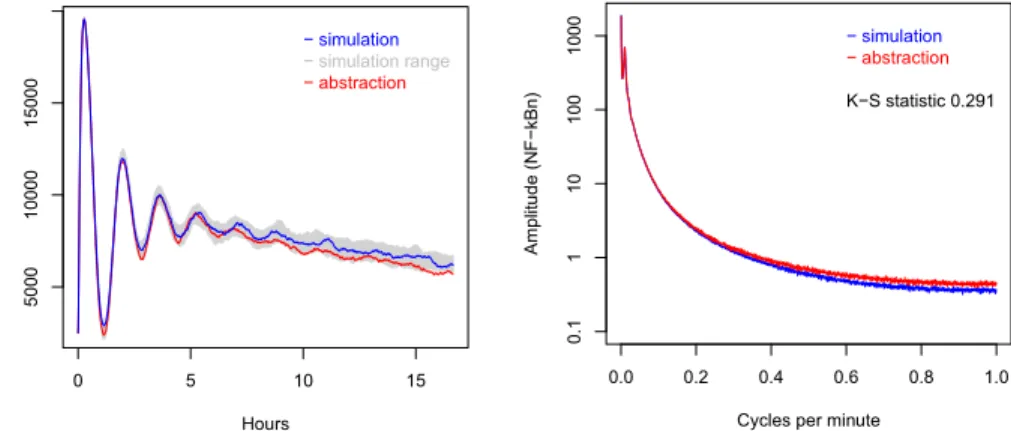
Figure 3. Traces of NF-kBn generated by simulation and abstraction.
Figure 4.Average spectra of simulation and abstraction of NF-kBn.
Since we wish to judge our abstraction with frequency domain analysis, we construct a simple process that generates sampled traces directly. This is suffi-cient to reveal the potential and shortfalls of the approach. We assume a train-ing set of M sampled simulation traces of the output variable of a subsystem, denoted ∪Mj=1(x(j)n )N−1n=0, where x
(j)
n is the nth sample of variable x in
simula-tion trace j. From this we construct a sequence of Gaussian random variables (Xn)Nn=1−1, where Xn ∼ N (Meanj∈{1,...M }(x(j)n − x(j)n−1), Variancej∈{1,...,M }(x(j)n −
x(j)n−1)). Each Xnthus models the change in values from sample n−1 to sample n.
A trace (y)Nn=0−1 may be generated from this abstraction by setting y0= x0(the
initial value) and iteratively calculating yn = yn−1+ ξn, where ξn is a sample
from Xn.
To judge the performance of our abstraction we measure the K-S distance between empirical distributions generated by the original system and by the Gaussian processes. We then compare this with the K-S distance between two empirical distributions generated by the original system (the ‘self distance’). In this investigation all distributions contain 100 traces. With infinitely large distri-butions the expected self distance is zero, but the random variation between finite
distributions causes the value to be higher. With 100 traces the self distances for p53a and NF-kBn are typically 0.02± 0.01. The K-S distances between the Gaussian process abstractions and empirical distributions of simulations form the original systems are typically 0.03 for p53a and 0.3 for NF-kBn. Using this metric, the p53a abstraction is almost indistinguishable from the original, but the abstraction for NF-kBn is not adequate. Figs. 3 and 4 illustrate the perfor-mance of the Gaussian process abstraction for NF-kBn. At this scale the p53a abstraction is visually indistinguishable from the original and is therefore not shown.
5
Challenges and Prospects
Empirical distribution abstractions are simple to construct, provide sample traces that are correct with respect to the causality of the systems they abstract, but are memory-intensive. In contrast, Gaussian processes offer a memory-efficient away to abstract external systems, but do not implicitly guarantee correct causality and their parameters must be learned from no fewer simulations than would be required for an empirical distribution. Despite this, Gaussian processes seem to offer the greatest potential for development, as a result of their scalability.
Our preliminary results suggest that it may be possible to create very good abstractions with Gaussian processes, but that our current simplistic approach will not in general be adequate. Our ongoing work will therefore investigate more sophisticated processes, together with ways to guarantee that their behaviour re-spects the causality of the systems they abstract. Their increased complexity will necessarily entail more sophisticated learning techniques, whose computational cost must also be included when considering efficiency.
A substantial future challenge is to adapt our techniques to systems with bidirectional communication between components. In this context empirical dis-tributions are unlikely to be adequate, since the abstractions would be required to change in response to input signals. One plausible approach is to construct Gaussian processes parametrised by functions of input signals.
References
1. C. Baier, B. Haverkort, H. Hermanns, and J. Katoen. Model-checking algorithms for continuous-time markov chains. Software Engineering, IEEE Transactions on, 29(6):524–541, 2003.
2. A. Basu, S. Bensalem, M. Bozga, B. Caillaud, B. Delahaye, and A. Legay. Sta-tistical abstraction and model-checking of large heterogeneous systems. In Formal Techniques for Distributed Systems, pages 32–46. Springer, 2010.
3. A. Biere, A. Cimatti, E. Clarke, and Y. Zhu. Symbolic model checking without BDDs. In W. Cleaveland, editor, Tools and Algorithms for the Construction and Analysis of Systems, volume 1579 of LNCS, pages 193–207. Springer, 1999. 4. L. Bortolussi and G. Sanguinetti. Learning and designing stochastic processes from
logical constraints. In K. Joshi, M. Siegle, M. Stoelinga, and P. R. D’Argenio, editors, Quantitative Evaluation of Systems, volume 8054 of LNCS, pages 89–105. Springer, 2013.
5. J. R. Burch, E. M. Clarke, K. L. McMillan, D. L. Dill, and L.-J. Hwang. Symbolic model checking: 1020states and beyond. Information and computation, 98(2):142– 170, 1992.
6. E. M. Clarke, E. A. Emerson, and J. Sifakis. Model checking: algorithmic verifica-tion and debugging. Commun. ACM, 52(11):74–84, Nov. 2009.
7. E. M. Clarke, O. Grumberg, and D. E. Long. Model checking and abstraction. ACM Transactions on Programming Languages and Systems (TOPLAS), 16(5):1512– 1542, 1994.
8. P. Cousot and R. Cousot. Abstract interpretation: a unified lattice model for static analysis of programs by construction or approximation of fixpoints. In Proceedings of the 4th ACM SIGACT-SIGPLAN symposium on Principles of programming languages, pages 238–252. ACM, 1977.
9. E. W. Dijkstra. Guarded commands, nondeterminacy and formal derivation of programs. Commun. ACM, 18:453–457, August 1975.
10. M. Gibson and J. Bruck. Efficient exact stochastic simulation of chemical systems with many species and many channels. J. of Physical Chemistry A, 104:1876, 2000. 11. D. Gillespie. Stochastic simulation of chemical kinetics. Annual Review of Physical
Chemistry, 58(1):35–55, 2007.
12. D. T. Gillespie. A general method for numerically simulating the stochastic time evolution of coupled chemical reactions. Journal of Computational Physics, 22(4):403 – 434, 1976.
13. D. T. Gillespie. A rigorous derivation of the chemical master equation. Physica A, 188:404–425, 1992.
14. P. Godefroid. Using partial orders to improve automatic verification methods. In Computer-Aided Verification, pages 176–185. Springer, 1991.
15. J. Heath and et al. Probabilistic model checking of complex biological pathways. Theoretical Computer Science, 391:239–257, 2008.
16. M. Hinchey and L. Coyle. Evolving critical systems. In Engineering of Computer Based Systems (ECBS), 2010 17th IEEE International Conference and Workshops on, pages 4–4, March 2010.
17. A. Ihekwaba and S. Sedwards. Communicating oscillatory networks: frequency domain analysis. BMC Systems Biology, 5(1):203, 2011.
18. C. Jegourel, A. Legay, and S. Sedwards. Importance splitting for statistical model checking rare properties. In N. Sharygina and H. Veith, editors, Computer Aided Verification, volume 8044 of LNCS, pages 576–591. Springer, 2013.
19. J. G. Kemeny, A. W. Knapp, and J. L. Snell. Denumerable markov chains. Springer, 1976.
20. M. Okamoto. Some inequalities relating to the partial sum of binomial probabili-ties. Annals of the Institute of Statistical Mathematics, 10:29–35, 1959.
21. A. N. Pettitt and M. A. Stephens. The Kolmogorov-Smirnov Goodness-of-Fit Statistic with Discrete and Grouped Data. Technometrics, 19(2):205–210, 1977. 22. C. E. Rasmussen and C. K. I. Williams. Gaussian Processes for Machine Learning.
The MIT Press, 2006.
23. S. Sedwards. A Natural Computation Approach To Biology: Modelling Cellular Processes and Populations of Cells With Stochastic Models of P Systems. PhD thesis, University of Trento, 2009.
24. J. M. G. Vilar, H. Y. Kueh, N. Barkai, and S. Leibler. Mechanisms of noise-resistance in genetic oscillators. Proceedings of the National Academy of Sciences, 99(9):5988–5992, 2002.
25. A. Wald. Sequential Tests of Statistical Hypotheses. Annals of Mathematical Statistics, 16(2):117–186, 1945.
A
Model of Coupled Oscillatory Systems
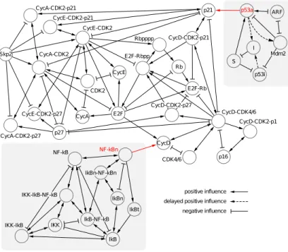
Fig. 5 illustrates the direct effect that one chemical species in the model has on another. Each node represents a state variable, whose value records the instan-taneous number of molecules of a chemical species. The edges in the graph are directional, having a source and destination node. Influence that acts in both directions is represented by a bi-directional edge. Positive influence implies that increasing the number of source molecules will increase the number of destina-tion molecules. The presence of an edge in the diagram indicates the existence of a command in which the source species variable appears in the rate and the destination species variable appears in the action. The variables that we use to abstract the external systems, namely p53a and NF-kBn, are highlighted in red.
Figure 5.Direct influence of variables in the case study. External systems are shown on grey backgrounds. Variables in red are used in abstractions.
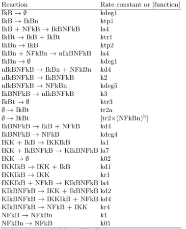
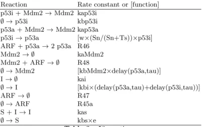
The precise technical details of the model are given in Tables 1 to 5. Table 2 gives the reaction scheme of the core system (the cell cycle). Tables 1 and 3 contain the reactions schemes of the external systems (NF-κB and p53, respec-tively). Table 4 gives the initial numbers of molecules of each species and Table 5 gives the values of the constants used.
The model is given in terms of chemical reactions for compactness and to be compatible with previous work on these systems. Reactions have the form
reactants→ products, where reactants and products are possibly empty multisets of chemical species, described by the syntax∅ | S { “+” S }, in which ∅ denotes the empty multiset and S is the name of a chemical species. The semantics of reactions assumes that the system contains a multiset of molecules. A reaction is enabled if reactants is a subset of this multiset. An enabled reaction is executed by removing reactants from the system and simultaneously adding products.
The rate at which a reaction is executed is stochastic. The majority of the reactions in our model are ‘elemental’ [11], working by ‘mass action kinetics’ according to fundamental physical laws [13]. Hence, under the assumption that the system is ‘well stirred’ [13], the rate at which a reaction is executed is given by the product of some rate constant k and the number of ways that reactants may be removed from the system. Elemental reactions in our model are thus converted to commands according to the following table.
Reaction pattern Command (guard, rate, action) ∅ → A (true, k, A = A + 1) A→ B (A > 0, kA, A = A− 1; B = B + 1) A→ B + C (A > 0, kA, A = A− 1; B = B + 1; C = C + 1) A + B→ C (A > 0∧ B > 0, kAB, A = A − 1; B = B − 1; C = C + 1) A + B→ C + D (A > 0 ∧ B > 0, kAB, A = A − 1; B = B − 1; C = C + 1; D = D + 1)
A few of the reactions are abstractions of more complex mechanisms, using Michaelis-Menten dynamics, Hill coefficients or delays. The semantics of their execution is the same, so the guard and action given above are correct, but the rate is given by an explicit function. Delays appear in the rate as a function of a molecular species S and a delay time τ . The value of this function at time t is the number of molecules of S at time t− τ.
The reaction rate constants and initial values have been inferred using ODE models that consider concentrations, rather than numbers of molecules. To con-vert the initial concentrations to molecules, they must be multiplied by a dis-cretisation constant, alpha, having the dimensions of volume. Specifically, alpha is the product of Avogadro’s number and the volume of a mammalian cell. The rate constants must also be transformed to work with numbers of molecules. The rate constants of reactions of the form∅ → · · · must be multiplied by alpha. The rate constants of reactions of the form A + B→ · · · must be divided by al-pha. The rate constants of reactions of the form A→ · · · may be used unaltered. In the case of explicit functions that are the product of a rate constant and a number of molecules raised to some power h, the value of the constant must be divided by alphah−1.
Reaction Rate constant or [function]
IkB → ∅ kdeg1
IkB → IkBn ktp1 IkB + NFkB → IkBNFkB la4 IkBt → IkB + IkBt ktr1 IkBn → IkB ktp2 IkBn + NFkBn → nIkBNFkB la4
IkBn → ∅ kdeg1 nIkBNFkB → IkBn + NFkBn kd4 nIkBNFkB → IkBNFkB k2 nIkBNFkB → NFkBn kdeg5 IkBNFkB → nIkBNFkB k3 IkBt → ∅ ktr3 ∅ → IkBt tr2a ∅ → IkBt [tr2×(NFkBn)h] IkBNFkB → IkB + NFkB kd4 IkBNFkB → NFkB kdeg4 IKK + IkB → IKKIkB la1 IKK + IkBNFkB → KIkBNFkB la7
IKK → ∅ k02
IKKIkB → IKK + IkB kd1 IKKIkB → IKK kr1 IKKIkB + NFkB → KIkBNFkB la4 KIkBNFkB → IKK + IkBNFkB kd2 KIkBNFkB → IKKIkB + NFkB kd4 KIkBNFkB → NFkB + IKK kr4 NFkB → NFkBn k1 NFkBn → NFkB k01
Reaction Rate constant or [function]
CycDCDK46 → CDK46 R1
CycDCDK46 + p16 → CycDCDp16 R29 CycDCDK46 + p27 → CycDCDp27 R6 CycDCDK46 → CDK46 + CycD R21b CycD + CDK46 → CycDCDK46 R21a
CDK46 → ∅ R32
CycACDK2 + E2F → CycACDK2 R15
∅ → E2F R43
E2F → E2F + E2F R42
CycE → ∅ R26
E2F → CycE + E2F R2
CycECDK2 → CDK2 R3
CycECDK2 → CDK2 + CycE R24b CDK2 + CycE → CycECDK2 R24a CDK2 + CycA → CycACDK2 R25a
CDK2 → ∅ R33
CycA → ∅ R27
E2F → CycA + E2F R4
CycACDK2 → CDK2 R5 CycACDK2 → CycA + CDK2 R25b p27 + CycECDK2 → CycECDp27 R7 p27 + CycACDK2 → CycACDp27 R8 ∅ → p27 R20 CycECDp27 + Skp2 → Skp2 + CycECDK2 R9 CycACDp27 + Skp2 → Skp2 + CycACDK2 R10 Skp2 → ∅ R34 ∅ → Skp2 R31 Rb → ∅ R18 Rb + E2F → E2FRb R11 ∅ → Rb R17 Rbpppp → Rb R16
CycDCDK46 + E2FRb → E2FRbpp + CycDCDK46 R12 CycDCDp27 + E2FRb → E2FRbpp + CycDCDp27 R13 CycDCDp21 + E2FRb → E2FRbpp + CycDCDp21 R41 E2FRbpp + CycECDK2 → CycECDK2 + Rbpppp + E2F R14
CycDCDp16 → p16 R19
p16 → ∅ R23
∅ → p16 R28
CycD → ∅ R22
E2F → CycD + E2F R44
∅ → CycD R30a
p21 + CycDCDK46 → CycDCDp21 R35a p21 + CycECDK2 → CycECDp21 R36a p21 + CycACDK2 → CycACDp21 R37a
∅ → p21 R40a CycDCDp21 → p21 + CycDCDK46 R35b CycECDp21 → p21 + CycECDK2 R36b Skp2 + CycECDp21 → CycECDK2 + Skp2 R38 CycACDp21 → p21 + CycACDK2 R37b Skp2 + CyCACDp21 → CycACDK2 + Skp2 R39 ∅ → CycD [R30b×(NFkBn)h] p53a → p21 + p53a R40b
Reaction Rate constant or [function] p53i + Mdm2 → Mdm2 kap53i
∅ → p53i kbp53i p53a + Mdm2 → Mdm2 kap53a
p53i → p53a [w×(Sn/(Sn+Ts))×p53i] ARF + p53a → 2 p53a R46
Mdm2 → ∅ kaMdm2 Mdm2 + ARF → ∅ R48 ∅ → Mdm2 [kbMdm2×delay(p53a,tau)] I → ∅ kai ∅ → I [kbi×(delay(p53a,tau)+delay(p53i,tau))] ARF → ∅ R47 ∅ → ARF R45a S + I → I kas ∅ → S kbs×e Table 3.p53 reactions.
Species Amount Species Amount p53i 0 CycECDK2 0
p53a 0.1×alpha CDK2 2.0×alpha Mdm2 0.15×alpha CycA 0
I 0.1×alpha CycACDK2 0
S 0 p27 1.0×alpha
ARF 0 CycDCDp27 0.001×alpha IkB 0 CycECDp27 0
IkBn 0 CycACDp27 0
nIkBNFkB 0 Skp2 1.0×alpha IkBt 0 Rb 1.0×alpha IkBNFkB 0.2×alpha E2FRb 1.95×alpha IKK 0.2×alpha E2FRbpp 1.0×10⁻³×alpha
IKKIkB 0 Rbpppp 1.02×alpha KIkBNFkB 0 CycDCDp16 1.0×10⁻⁵×alpha
NFkB 0 p16 1.0×alpha NFkBn 0.025×alpha CycD 0 CycDCDK46 0 p21 0 CDK46 5.0×alpha CycDCDp21 0 E2F 0 CycECDp21 0 CycE 0 CycACDp21 0
Name Value Name Value Name Value alpha 100000 R8 7.0 × 10⁻²/alpha R35b 5.0 × 10⁻³
h 2 R9 0.225/alpha R36a 1.0 × 10⁻²/alpha
kdeg1 0.16 R10 2.5 × 10⁻³/alpha R36b 1.75 × 10⁻⁴
ktp1 0.018 R11 5.0 × 10⁻⁵/alpha R37a 7.0 × 10⁻²/alpha
ktp2 0.012 R12 1.0 × 10⁻⁴/alpha R37b 1.75 × 10⁻⁴
ktr1 0.2448 R13 1.0 × 10⁻²/alpha R38 0.225/alpha
kd4 0.00006 R14 0.073/alpha R39 2.5 × 10⁻³/alpha
la1 0.1776/alpha R15 0.022/alpha R40a 5.0 × 10⁻⁵×alpha
kd1 0.000888 R16 5.0 × 10⁻⁸ R40b 1.0 × 10⁻³
la4 30/alpha R17 5.0 × 10⁻⁵×alpha R41 1.0 × 10⁻²/alpha
k2 0.552 R19 5.0 × 10⁻²/alpha R42 1.0 × 10⁻⁴
k3 0.00006 R20 1.0 × 10⁻⁴×alpha R43 5.0 × 10⁻⁵×alpha
tr2a 0.000090133×alpha R21a 2.0 × 10⁻³/alpha R44 3.0 × 10⁻⁴
ktr3 0.020733 R21b 8.0 × 10⁻³ R45a 8.0 × 10⁻⁵×alpha
tr2 0.5253/alpha(h−1) R22 7.5 × 10⁻³ R45b 0.008
kdeg4 0.00006 R23 5.0 × 10⁻³ R46 2.333 × 10⁻⁵/alpha
kdeg5 0.00006 R24a 8.0 × 10⁻³/alpha R47 0.01167
la7 6.06/alpha R24b 3.9 × 10⁻³ R48 1.167 × 10⁻⁵/alpha
kd2 0.095 R25a 8.0 × 10⁻³/alpha kbp53i 0.015×alpha
kr1 0.012 R25b 4.0 × 10⁻³ kbMdm2 0.01667
kr4 0.22 R26 2.5 × 10⁻³ kap53i 2.333/alpha
k1 5.4 R27 5.0 × 10⁻⁴ kaMdm2 0.01167
k01 0.0048 R28 2.0 × 10⁻⁴×alpha tau 80
k02 0.0072 R29 5.0 × 10⁻⁴/alpha kap53a 0.02333/alpha
R1 5.0 × 10⁻⁶ R30a 0.004×alpha kas 0.045/alpha
R2 4.5 × 10⁻³ R30b 0.9961/alpha(h−1)kbi 0.01667
R3 5.0 × 10⁻³ R31 5.0 × 10⁻⁴×alpha kai 0.01167
R4 2.5 × 10⁻³ R32 8.0 × 10⁻⁴ kbs 0.015×alpha
R5 5.0 × 10⁻⁴ R33 8.0 × 10⁻⁴ e 1
R6 5.0 × 10⁻⁴/alpha R34 9.0 × 10⁻⁴ n 4
R7 1.0 × 10⁻²/alpha R35a 5.0 × 10⁻⁴/alpha w 11.665
Ts 1 × alphan