Fractal inverse problem: an analytical approach

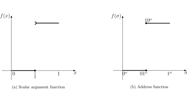
(3) generally holds for hyperbolic maps, one can apply exactly the same technique to non-linear cookie-cutters. Figure 2a) displays the 1D map extracted from the wavelet transform

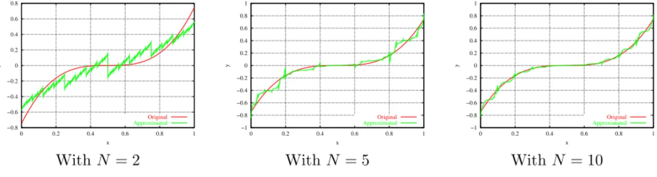
To mitigate the phenomenon of overfitting we can either regularize by adding a penalty on the model in the cost function which would penalize the too strong oscillations

L’archive ouverte pluridisciplinaire HAL, est destinée au dépôt et à la diffusion de documents scientifiques de niveau recherche, publiés ou non, émanant des

Therefore, there is no reuse within the activities of modelling ontology axioms, choosing ontologies for use in data graphs, and creating SHACL shapes to validate the data graph..

In the second step the network is characterized regarding: (i) the QSD of the provided objects, (ii) the kind of connections, and (iii) the new composed features of angle, convexity

The loss expression in rectangular regions can be both used for the computation of the macroscopic classical loss component (i.e. currents flowing at the scale of the

L’archive ouverte pluridisciplinaire HAL, est destinée au dépôt et à la diffusion de documents scientifiques de niveau recherche, publiés ou non, émanant des

We discuss an approach based on the model space theory which brings some integral representations for functions in R n and their derivatives.. Using this approach we obtain L p

References

[AKH97] Toshimizu Abiko, Masayuki Kawamata, and Tatsuo Higuchi. An efficient algorithm for solving inverse problems of fractal images using the complex moment method. In Proceed-ings of IEEE International Workshop on Intelligent Signal Processing and Communication Systems, volume 1, pages S12.4.1–S12.4.6. November 1997.
[Bar88] Michael Barnsley. Fractals everywhere. Academic Press, 1988.
[BD85] M.F Barnsley and S. Demko. Iterated function systems and the global construction of fractals. Proceeding of the Royal Society of London Ser A399, pages 243–275, 1985. [Ber97] K Berkner. A wavelet-based solution to the inverse problem for fractal interpolation
functions. In Tricot L´evy-V´ehel, Lutton, editor, Fractals in engineering’97, pages 81–92. Springer Verlag, 1997.
[BV91] R M Bolle and B C Vemuri. On Three-Dimensional Surface Reconstruction Methods. IEEE Transactions on Pattern Analysis and Machine Intelligence, 13(1):1–13, January 1991.
(22)
[CK94] K. Culik and J. Karhum¨aki. Finite automata computing real functions. SIAM Journal on Computing, 23(4):789–814, 1994.
[CK95] K. Culik and J. Kari. Inference Algorithms for WFA and Image Compression. In Yuval Fisher, editor, Fractal Image Encoding and Compression, pages 235–320. Springer-Verlag, 1995.
[DL93] Ingrid Daubechies and Jeffrey C. Lagarias. Two-scale difference equations II. local regu-larity, infinite products of matrices and fractals. SIAM. J. Math. Anal., 23(4):1031–1079, July 1993.
[Edg90] Gerald A. Edgar. Measure, Topology, and Fractal Geometry. Springer Verlag, 1990. [FX98] Zhigang Feng and Heping Xie. On Stability of Fractal Interpolation. Fractals, 6(3):269–
273, 1998.
[GB93] A Gupta and R Bajcsy. Volumetric segmentation of range images of 3D objects using superquadrics models. CVGIP: Image understanding, 58(3):302–326, November 1993. [GGN00] B Girod, G Greiner, and H Niemann, editors. Principles of 3D Image Analysis and
Synthesis. Kluwer Academic Publishers, 2000.
[GTB00] Eric Gu´erin, Eric Tosan, and Atilla Baskurt. Fractal coding of shapes based on a projected IFS model. In ICIP 2000, volume II, pages 203–206, September 2000.
[GTB01a] Eric Gu´erin, Eric Tosan, and Atilla Baskurt. A fractal approximation of curves. Fractals, 9(1):95–103, March 2001.
[GTB01b] Eric Gu´erin, Eric Tosan, and Atilla Baskurt. Fractal Approximation of Surfaces based on projected IFS attractors. In Proceedings of EUROGRAPHICS’2001, short presentations, 2001.
[GTB02] Eric Gu´erin, Eric Tosan, and Atilla Baskurt. Modeling and approximation of fractal surfaces with projected IFS attractors. In M. M. Novak, editor, Emergent Nature. World Scientific, 2002.
[GTB03] Eric Gu´erin, Eric Tosan, and Atilla Baskurt. Fractal compression of images with projected ifs. In PCS’2003, Picture Coding Symposium, St Malo, April 2003.
[Gu´e02] Eric Gu´erin. Approximation fractale de courbes et de surfaces. Th`ese de doctorat, Uni-versit´e Claude Bernard Lyon 1, December 2002.
[Jac92] A E Jacquin. Image coding based on a fractal theory of iterated contractive image trans-formations. IEEE Trans. on Image Processing, 1:18–30, January 1992.
[LLVC+95] Evelyne Lutton, Jacques L´evy-V´ehel, Guillaume Cretin, Philippe Glevarec, and C´edric Roll. Mixed IFS : resolution of the inverse problem using genetic programming. Rapport de recherche 2631, Institut National de Recherche en Informatique et en Automatique, August 1995. Programme 5.
[PFTV93] W. H. Press, B. P. Flannery, S. A. Teukolsky, and W. T. Vetterling. Numerical Recipes in C : The Art of Scientific Computing, chapter Nonlinear Models. Cambridge University Press, 1993.
(23)
[PM87] H. Prautzsch and Charles A. Micchelli. Computing curves invariant under halving. Com-puter Aided Geometric Design, (4):133–140, 1987.
[SDG95] Z R Struzik, E H Dooijes, and F C A Groen. The solution of the inverse fractal problem with the help of wavelet decomposition. In M M Novak, editor, Fractals reviews in the natural and applied sciences, pages 332–343. Chapman and Hall, February 1995.
[TM91] D Terzopoulos and D Metaxas. Dynamic 3D models with local and global deformations: deformable superquadrics. IEEE Transactions on Pattern Analysis and Machine Intelli-gence, 13(7):703–714, July 1991.
[VS99] Edward R. Vrscay and Dietmar Saupe. Can one break the collage barrier in fractal image coding. In Dekking, Vehel, Lutton, and Tricot, editors, Fractals : theory and applications in engineering, pages 307–323. Springer, 1999.
[ZT96a] Chems Eddine Zair and Eric Tosan. Fractal modeling using free form techniques. Computer Graphics Forum, 15(3):269–278, August 1996. EUROGRAPHICS’96 Conference issue. [ZT96b] Chems Eddine Zair and Eric Tosan. Fractal modeling using free form techniques. Computer
Graphics Forum, 15(3):269–278, August 1996. EUROGRAPHICS’96 Conference issue. [ZT97a] Chems Eddine Zair and Eric Tosan. Computer Aided Geometric Design with IFS
tech-niques. In M M Novak and T G Dewey, editors, Fractals Frontiers, pages 443–452. World Scientific Publishing, April 1997.
[ZT97b] Chems Eddine Zair and Eric Tosan. Unified IFS-based Model to Generate Smooth or Fractal Forms. In A. Le M´ehaut´e, C. Rabut, and L. L. Schumaker, editors, Surface Fitting and Multiresolution Methods, pages 335–344. Vanderbilt University Press, Nashville, TN, 1997.
Figure
Figure 1: Comparison between scalar argument functions and address functions
Figure 2: Example of a projected IFS curve
Figure 3: Surface modeling with projected IFS quadtree
Figure 4: Approximation of a cubic polynomial curve (1000 points)
+3
Références
Documents relatifs