HAL Id: hal-01628798
https://hal.inria.fr/hal-01628798
Submitted on 6 Nov 2017
HAL is a multi-disciplinary open access
archive for the deposit and dissemination of
sci-entific research documents, whether they are
pub-lished or not. The documents may come from
teaching and research institutions in France or
L’archive ouverte pluridisciplinaire HAL, est
destinée au dépôt et à la diffusion de documents
scientifiques de niveau recherche, publiés ou non,
émanant des établissements d’enseignement et de
recherche français ou étrangers, des laboratoires
Locality
Oleksandr Zinenko, Sven Verdoolaege, Chandan Reddy, Jun Shirako, Tobias
Grosser, Vivek Sarkar, Albert Cohen
To cite this version:
Oleksandr Zinenko, Sven Verdoolaege, Chandan Reddy, Jun Shirako, Tobias Grosser, et al.. Unified
Polyhedral Modeling of Temporal and Spatial Locality. [Research Report] RR-9110, Inria Paris. 2017,
pp.41. �hal-01628798�
0249-6399 ISRN INRIA/RR--9110--FR+ENG
RESEARCH
REPORT
N° 9110
October 2017Modeling of Temporal
and Spatial Locality
Oleksandr Zinenko, Sven Verdoolaege, Chandan Reddy, Jun Shirako,
Tobias Grosser, Vivek Sarkar, Albert Cohen
RESEARCH CENTRE PARIS
Oleksandr Zinenko
*, Sven Verdoolaege
, Chandan Reddy
*, Jun
Shirako
§, Tobias Grosser
¶, Vivek Sarkar
§, Albert Cohen
*Project-Team Parkas
Research Report n° 9110 — October 2017 — 37 pages
Abstract: Despite decades of work in this area, the construction of effective loop nest optimizers and parallelizers continues to be challenging due to the increasing diversity of both loop-intensive application workloads and complex memory/computation hierarchies in modern processors. The lack of a systematic approach to optimizing locality and parallelism, with a well-founded data locality model, is a major obstacle to the design of optimizing compilers coping with the vari-ety of software and hardware. Acknowledging the conflicting demands on loop nest optimization, we propose a new unified algorithm for optimizing parallelism and locality in loop nests, that is capable of modeling temporal and spatial effects of multiprocessors and accelerators with deep memory hierarchies and multiple levels of parallelism. It orchestrates a collection of parameter-izable optimization problems for locality and parallelism objectives over a polyhedral space of semantics-preserving transformations. The overall problem is not convex and is only constrained by semantics preservation. We discuss the rationale for this unified algorithm, and validate it on a collection of representative computational kernels/benchmarks.
Key-words: polyhedral model, loop nest optimization, automatic parallelization
*Inria Paris and DI, ´Ecole Normale Sup´erieure KU Leuven
PSL Research University §Rice Univresity
R´esum´e : Malgr´e les d´ecennies de travail dans ce domaine, la construction de compila-teurs capables de parall´eliser et optimiser les nids de boucle reste un probl`eme difficile, dans le contexte d’une augmentation de la diversit´e des applications calculatoires et de la complexit´e de la hi´erarchie de calcul et de stockage des processeurs modernes. L’absence d’une m´ethode syst´ematique pour optimiser la localit´e et le parall´elisme, fond´ee sur un mod`ele de localit´e des donn´ees pertinent, constitue un obstacle majeur pour prendre en charge la vari´et´e des besoins en optimisation de boucles issus du logiciel et du mat´eriel. Dans ce contexte, nous proposons un nou-vel algorithme unifi´e pour l’optimisation du parall´elisme et de la localit´e dans les nids de boucles, capable de mod´eliser les effets temporels et spatiaux des multiprocesseurs et acc´el´erateurs com-portant des hi´erarchies profondes de parall´elisme et de m´emoire. Cet algorithme coordonne la r´esolution d’une collection de probl`emes d’optimisation param´etr´es, portant sur des objec-tifs de localit´e ou et de parall´elisme, dans un espace poly´edrique de transformations pr´eservant la s´emantique du programme. La conception de cet algorithme fait l’objet d’une discussion syst´ematique, ainsi que d’une validation exp´erimentale sur des noyaux calculatoires et bench-marks repr´esentatifs.
Mots-cl´es : mod`ele poly´edrique, transformations de nids de boucles, parall´elisation automa-tique
1
Introduction
Computer architectures continue to grow in complexity, stacking levels of parallelism and deepen-ing their memory hierarchies to mitigate physical bandwidth and latency limitations. Harnessdeepen-ing more than a small fraction of the performance offered by such systems is a task of ever growing difficulty. Optimizing compilers transform a high-level, portable, easy-to-read program into a more complex but efficient, target-specific implementation. Achieving performance portability is even more challenging: multiple architectural effects come into play that are not accurately modeled as convex optimization problems, and some may require mutually conflicting program transformations. In this context, systematic exploration of the space of semantics-preserving, parallelizing and optimizing transformations remains a primary challenge in compiler construc-tion.
Loop nest optimization holds a particular place in optimizing compilers as, for computational programs such as those for scientific simulation, image processing, or machine learning, a large part of the execution time is spent inside nested loops. Research on loop nest transformations has a long history Wolfe (1995); Kennedy and Allen (2002). Much of the past work focused on specific transformations, such as fusion Kennedy and McKinley (1993), interchange Allen and Kennedy (1984) or tiling Wolfe (1989); Irigoin and Triolet (1988), or specific objectives, such as parallelization Wolfe (1986) or vectorization Allen and Kennedy (1987).
The polyhedral framework of compilation introduced a rigorous formalism for representing and operating on the control flow, data flow, and storage mapping of a growing class of loop-based programs Feautrier and Lengauer (2011). It provides a unified approach to loop nest optimization, offering precise relational analyses, formal correctness guarantees and the ability to perform complex sequences of loop transformations in a single optimization step by using powerful code generation/synthesis algorithms. It has been a major force driving research on loop transformations in the past decade thanks to the availability of more generally applicable algorithms, robust and scalable implementations, and embeddings into general or domain-specific compiler frameworks Pop et al. (2006); Grosser et al. (2012). Loop transformations in polyhedral frameworks are generally abstracted by means of a schedule, a multidimensional relation from iterative instances of program statements to logical time. Computing the most profitable valid schedule is the primary goal of a polyhedral optimizer. Feautrier’s algorithm computes mini-mum delay schedules Feautrier (1992b) for arbitrary nested loops with affine bounds and array subscripts. The Pluto algorithm revisits the method to expose coarse-grain parallelism while improving temporal data locality Bondhugula et al. (2008b, 2016). However, modern complex processor architectures have made it imperative to model more diverse sources of performance; deep memory hierarchies that favor consecutive accesses—cache lines on CPUs, memory coa-lescing on GPUs—are examples of hardware capabilities which must be exploited to match the performance of hand-optimized loop transformations.
There has been some past work on incorporating knowledge about consecutive accesses into a polyhedral optimizer, mostly as a part of transforming programs for efficient vectorization Tri-funovic et al. (2009); Vasilache et al. (2012); Kong et al. (2013). However, these techniques restrict the space of schedules that can be produced; we show that these restrictions miss poten-tially profitable opportunities involving schedules with linearly dependent dimensions or those obtained by decoupling locality optimization and parallelization. In addition, these techniques model non-convex optimization problems through the introduction of additional discrete (inte-ger, boolean) variables and of bounds on coefficients. These ad-hoc bounds do not practically impact the quality of the results, but remain slightly unsatisfying from a mathematical modeling perspective. Finer architectural modeling such as the introduction of spatial effects also pushes for more discrete variables, requiring extra algorithmic effort to keep the dimensional growth
un-der control. A different class of approaches relies on a combination of polyhedral and traditional, syntactic-level loop transformations. A polyhedral optimizer is set up for one objective, while a subsequent syntactic loop transformation addresses another objective. For example, PolyAST uses a polyhedral optimizer to improve locality through affine scheduling and loop tiling. After that, it applies syntactic transformations to expose different forms of parallelism Shirako et al. (2014). Prior to PolyAST, the pionneering Pluto compiler itself already relied on a heuristic loop permutation to improve spatial locality after the main polyhedral optimization aiming for parallelism and temporal locality Bondhugula et al. (2008b). Operating in isolation, the two optimization steps may end up undoing each other’s work, hitting a classical compiler phase ordering problem.
We propose a polyhedral scheduling algorithm that accounts for multiple levels of parallelism and deep memory hierarchies, and does so without imposing unnecessary limits on the space of possible transformations. Ten years ago, the Pluto algorithm made a significant contribution to the theory and practice of affine scheduling for locality and parallelism. Our work extends this frontier by revisiting the models and objectives in light of concrete architectural and microar-chitectural features, leveraging positive memory effects (e.g., locality) and avoiding the negative ones (e.g., false sharing). Our work is based on the contributions of the isl scheduler Verdoolaege and Janssens (2017). In particular, we formulate a collection of parameterizable optimization problems, with configurable constraints and objectives, that rely on the scheduler not insist-ing on the initial schedule rows beinsist-ing linearly independent for lower-dimensional statements in imperfectly nested loops. Our approach to locality-enhancing fusion builds on the “clustering” technique, also introduced in the isl scheduler, which allows for a precise intertwining of the iterations of different statements while maintaining the execution order within each loop, and we extend the loop sinking options when aligning imperfectly nested loops to the same depth. We address spatial effects by extending the optimization objective and by using linearly dependent dimensions in affine schedules that are out of reach of a more greedy polyhedral optimizer.
We design our algorithm as a template with multiple configuration dimensions. Its flexibility stems from a parameterizable scheduling problem and a pair of optimization objectives that can be interchanged during the scheduling process. As a result, our approach is able to produce in one polyhedral optimization pass schedules that previously required a combination of polyhedral and syntactic transformations. Since it remains within the polyhedral model, it can benefit from its transformation expressiveness and analysis power, e.g., to apply optimizations that a purely syntactic approach might not consider, or to automatically generate parallelized code for different accelerators from a single source.
2
Background
The polyhedral framework is based on a linear algebraic representation of the program parts that are “sufficiently regular”. It represents arithmetic expressions surrounded by loops and branches with conditions that are affine functions of outer loop iterators and runtime constants Feautrier and Lengauer (2011). These constants, referred to as parameters, may be unknown at compilation time and are treated symbolically. Expressions may read and write to multidimensional arrays with the same restrictions on the subscripts as on control flow. It has been the main driving power for research on loop optimization and parallelization in the last two decades Feautrier (1992b); Bastoul (2004); Bondhugula et al. (2008b); Grosser et al. (2012).
The polyhedral framework operates on individual executions of statements inside loops, or statement instances, which are identified by a named multidimensional vector, where the name identifies the statement and the coordinates correspond to iteration variables of the surrounding
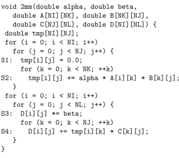
for (i = 0; i < N; ++i) for (j = 0; j < N; ++j) S: C[i][j] = 0.0; for (i = 0; i < N; ++i) for (j = 0; j < N; ++j) for (k = 0; k < N; ++k) R: C[i][j] += A[i][k] * B[k][j];
Figure 1: Naive implementation of matrix multiplication.
loops. The set of all named vectors is called the iteration domain of the statement. Iteration domains can be expressed as multidimensional sets constrained by Presburger formulas Pugh and Wonnacott (1994). For example, the code fragment in Figure 1 contains two statements, S and R with iteration domains DS(N ) = { S(i, j) | 0 ≤ i, j < N } and DR(N ) = { R(i, j, k) |
0 ≤ i, j, k < N } respectively. In this paper, we use parametric named relations as also used in iscc Verdoolaege (2011); note that the vectors in DS and DR are prefixed with the statement
name. Unless otherwise specified, we assume all values to be integer, i, j, · · · ∈ Z.
Polyhedral modeling of the control flow maps every statement instance to a multidimensional logical execution date Feautrier (1992b). The instances are executed following the lexicographic order of their execution dates. This mapping is called a schedule, typically defined by piecewise (quasi-)affine functions over the iteration domain TS(ppp) = { iii → ttt | { tj = φS,j(iii, ppp) } ∧ iii ∈
DS}, which are disjoint unions of affine functions defined on a finite partition of the iteration
domain. The use of quasi-affine functions allows integer division by constants. This form of schedule allows arbitrarily complex loop traversals and interleavings of statement instances. In this paper, xxx denotes a row vector and ~x denotes a column vector. Code motion transformations may be expressed either by introducing auxiliary dimensions Kelly and Pugh (1995) in the schedule or by using a schedule tree structure that directly encodes enclosure and statement-level ordering Verdoolaege et al. (2014). For example, the schedule that preserves the original execution order in Figure 1 can be expressed as TS(N ) = { S(i, j) → (t1, t2, t3, t4) | t1= 0 ∧ t2=
i ∧ t3 = j ∧ t4 = 0 }, TR(N ) = { R(i, j, k) → (t1, t2, t3, t4) | t1 = 1 ∧ t2 = i ∧ t3 = j ∧ t4 = k }.
The first dimension is independent of the iteration domain and ensures that all instances of S are executed before any instance of R.
To preserve the program semantics during transformation, it is sufficient to ensure that the order of writes and reads of the same memory cell remains the same Kennedy and Allen (2002). First, accesses to array elements (a scalar being a zero-dimensional array) are expressed as multidimensional relations between iteration domain points and named cells. For example, the statement S has one write access relation Awrite
S→C = { S(i, j) → C(a1, a2) | a1= i∧a2= j }. Second,
pairs of statement instances accessing the same array element where at least one access is a write are combined to define a dependence relation. For example, the dependence between statements S and R is defined by a binary relation PS→R = { S(i, j) → R(i0, j0, k) | i = i0∧ j = j0∧ (i, j) ∈
DS∧ (i0, j0, k) ∈ DR}. This approach relates all statement instances accessing the same memory
cell and is referred to as memory-based dependence analysis. It is possible to compute exact data flow given a schedule using the value-based dependence analysis Feautrier (1991). In this case, the exact statement instance that wrote the value before a given read is identified. For example, instances of R with k 6= 0 no longer depend on S: PS→R = { S(i, j) → R(i0, j0, k) | i = i0∧ j =
j0∧ k = 0 ∧ (i, j) ∈ DS∧ (i0, j0, k) ∈ DR}.
A dependence is satisfied by a schedule if all the statement instances in the domain of its relation are scheduled before their counterparts in the range of its relation, i.e., dependence
sources are executed before respective sinks. A program transformation is valid, i.e., preserves original program semantics, if all dependences are satisfied.
2.1
Finding Affine Schedules
Numerous optimization algorithms in the polyhedral framework define a closed form of all valid schedules and solve an optimization problem in that space. As they usually rely on integer programming, objective functions and constraints should be expressed as affine functions of iter-ation domain dimensions and parameters. Objectives may include: minimum latency Feautrier (1992b), parallelism Bondhugula et al. (2008b), locality Bondhugula et al. (2008a) and others.
Multidimensional affine scheduling aims to determine sequences of statement schedule func-tions of the form φSj = iii~cj+ ppp ~dj+ D where ~cj, ~dj, D are (vectors of) unknown integer values.
Each such affine function defines one dimension of a multidimensional schedule.
Dependence Distances, Dependence Satisfaction and Violation Consider the affine form (φR,j(iii0, ppp)−φS,j(iii, ppp)), defined for a dependence between S(iii) and R(iii0). This form represents
the distance between dependent statement instances. If the distance is positive, the dependence is strongly satisfied, or carried, by per-statement scheduling functions φ. If it is zero, the dependence is weakly satisfied. A dependence with a negative distance that was not carried by any previous scheduling function is violated and the corresponding program transformation is invalid. For a schedule to be valid, i.e., to preserve the original program semantics, it is sufficient that it carries all dependences Kennedy and Allen (2002).
Farkas’ Lemma Note that the target form of the schedule function contains multiplication between unknown coefficients cccj, dddj, D and loop iterator variables iii that may take any value
within the iteration domain. This relation cannot be represented directly in a linear programming problem. Polyhedral schedulers usually rely on the affine form of Farkas’ lemma, a fundamental result in linear algebra that states that an affine form ccc~x + d is nonnegative everywhere in the (non-empty) set defined by A~x + ~b ≥ 0 iff it is a linear combination ccc~x + d ≡ λ0+ λλλ(A~x + ~b),
where λ0, λλλ ≥ 0. Applying Farkas’ lemma to the dependence distance relations and equating
coefficients on the left and right hand side of the equivalence gives us constraints on schedule coefficients cccj for the dependence to have non-negative distance, i.e., to be weakly satisfied by
the schedule function, in the iteration domains.
Permutable Bands A sequence of schedule functions is referred to as a schedule band. If all of these functions weakly satisfy the same set of dependences, they can be freely interchanged with each other without violating the original program semantics. Hence the band is permutable. Such bands satisfy the sufficient condition for loop tiling Irigoin and Triolet (1988) and are also referred to as tilable bands.
2.2
Feautrier’s Algorithm
Feautrier’s algorithm is one of the first to systematically compute a (quasi-)affine schedule if there exists exits one Feautrier (1992a,b). It produces minimal latency schedules. The general idea of the algorithm is to find the minimal number of affine scheduling functions by ensuring that each of them carries as many dependences as possible. Once all dependences have been carried by the outer loops, the statement instances inside each individual iteration can be computed in any order, including in parallel. Hence, Feautrier’s algorithm exposes inner, fine-graph parallelism.
Encoding Dependence Satisfaction Let us introduce an extra variable ek for each
depen-dence in the program. This variable is constrained by 0 ≤ ek ≤ 1 and by ek ≤ φRk,j(iii
0, ppp) −
φSk,j(iii, ppp) for all Sk(iii) → Rk(iii
0) in Pk⊆ P
Sk→Rk, with P
k a group of dependences between source
Sk and sink Rk. The condition ek = 1 holds iff the entire group of dependences Pk is carried by
the given schedule function.
Affine Transformations Feautrier’s scheduler proceeds by solving linear programming (LP) problems using a special lexmin objective. This objective was introduced in the PIP tool and results in the lexicographically smallest vector of the search space Feautrier (1988). Intuitively, lexmin first minimizes the foremost component of the vector and only then moves on to the next component. Thus it can optimize multiple criteria and establish preference among them.
The algorithm computes schedule functions that carry as many (groups of) dependences as possible by introducing a penalty for each non-carried group and by minimizing the penalty. The secondary criterion is to generate small schedule coefficients, typically decomposed into minimizing sums of parameter and schedule coefficients separately. These criteria are encoded in the LP problem as lexminX k (1 − ek), ns X j=1 np X i=1 dj,i, ns X j=1 dim DSj X i=1 cj,i, e1, e2. . . ek. . . (1)
where individual dj,i and cj,i for each statement are included in the trailing positions of the
vector in no particular order, np = dim ~p and ns is the number of statements. The search space
is constrained, using the Farkas lemma, to the values dj,i, cj,ithat weakly satisfy the dependences.
Dependences that are carried by the newly computed schedule function are removed from further consideration. The algorithm terminates when all dependences have been carried.
2.3
Pluto Algorithm
The Pluto algorithm is one of the core parallelization and optimization algorithms Bondhugula et al. (2008b). Multiple extensions have been proposed, including different search spaces Vasi-lache et al. (2012), specializations and cost functions for GPU Verdoolaege et al. (2013) and proofs of the existence of a solution Bondhugula et al. (2016).
Data Dependence Graph Level On a higher level, Pluto operates on the data dependence graph (DDG), where nodes correspond to statements and edges together with associated rela-tions define dependences between them. Strongly connected components (SCC) of the DDG correspond to the loops that should be preserved in the program after transformation Kennedy and Allen (2002). Note that one loop of the original program containing multiple statements may correspond to multiple SCCs, in which case loop distribution is allowed. For each compo-nent, Pluto computes a sequence of permutable bands of maximal depth. To form each band, it iteratively computes affine functions linearly independent from the already computed ones. Linear independence ensures the algorithm makes progress towards a complete schedule on each step. Carried dependences are removed only when it is no longer possible to find a new function that weakly satisfies all of them, which delimits the end of the permutable band. After remov-ing some dependences, Pluto recomputes the SCCs on the updated DDG and iterates until at least as many scheduling functions as nested loops are found and all dependences are carried. Components are separated by introducing an auxiliary dimension and scheduled by topological sorting.
Affine Transformation Level The affine transformation computed by Pluto is based on the observation that dependence distance (φR,j(iii0, ppp)−φS,j(iii, ppp)) is equal to the reuse distance, i.e., the
number of iterations of the given loop between successive accesses to the same data. Minimizing this distance will improve locality. Furthermore, a zero distance implies that the dependence is not carried by the loop (all accesses are made within the same iteration) and thus does not prevent its parallelization. Pluto uses Farkas’ lemma to define a parametric upper bound on the distance (φR,j(iii0, ppp) − φ
S,j(iii, ppp)) ≤ uuu~p + w, which can be minimized in an ILP problem as
lexmin u1, u2, . . . , unp, w, . . . , cS,1, . . .
where np = dim ~p, and cS,k are the coefficients of φS,j. The cS,k coefficients are constrained to
be represent a valid schedule, i.e., not violate dependences, using Farkas’ lemma. They are also restricted to have at least one strictly positive component along a basis vector of the null space of the current partial schedule, which guarantees linear independence. Note that it is sufficient to have a non-zero component rather than a strictly positive one, but avoiding a trivial solution with all components being zero may be computationally expensive Bondhugula et al. (2016). Fusion Auxiliary dimensions can be used not only to separate components, but also to group them together by assigning identical constant values to these dimensions. This corresponds to a loop fusion. By default, the Pluto implementation relies on the smart fusion heuristic that separates the DDG into a pair of subgraphs by cutting an edge, hence performing loop fission, based on how “far” in terms of original execution time the dependent instances are. Extensions exist to set up an integer programming problem to find auxiliary dimension constant values that maximize fusion between components while keeping the number of required prefetching streams limited Bondhugula et al. (2010a). Pluto also features the maximum fusion heuristic, which computes weakly connected components of the DDG and keeps statements together unless it is necessary to respect the dependence.
Tiling For each permutable band with at least two members, Pluto performs loop tiling after the full schedule has been computed. It is applied by inserting a copy of the band’s dimensions immediately before the band and modifying them to have a larger stride. The new dimensions correspond to tile loops and the original ones now correspond to point loops. Various tile shapes are supported through user-selected options. For the sake of simplicity, we hereinafter focus on rectangular tiles.
Differentiating Tile and Point Schedule The default tile construction uses identical sched-ules for tile and point loops. Pluto allows different schedsched-ules to be constructed using the following two post-affine modifications. First, a wavefront schedule allows parallelism to be exposed at the tile loop level. If the outermost schedule function of the band carries dependences, i.e., the corresponding loop is not parallel, then it may be replaced by the sum of itself with the follow-ing function, performfollow-ing a loop skewfollow-ing transformation. It makes the dependences previously carried by the second-outermost function to be carried by the outermost one instead, rendering the second one parallel. Such wavefronts can be constructed for one or all remaining dimensions of the band exposing different degrees of parallelism. Second, loop sinking allows some leverage for locality and vectorizability of point loops. Pluto chooses the point loop j that features the most locality using the heuristic based on scheduled access relations A ◦ T−1
j : Lj= nS· X i (2si+ 4li− 16oi) + 8v ! → max, (2)
where nS is the number of statements for which j-th schedule dimension is an actual loop rather
than a constant, si = 1 if the scheduled access Ai◦ T−1 features spatial locality and si = 0
otherwise; li = 1 if it yields temporal locality and li = 0 otherwise; oi = 1 if it does not yield
either temporal or spatial locality si = li = 0 and oi = 0 otherwise; and v = 1 if oi = 0 for
all i.1 Spatial locality is observed along j-th dimension if it appears in the last array subscript with a small stride and does not appear in previous subscripts: ai = f⊥tj(ttt) + g(uuu) + w, 1 ≤
i < na∧ ana = f⊥tj(ttt) + ktj+ g(uuu) + w, 1 ≤ k ≤ 4, na = dim(Dom A), where f⊥tj(ttt) denotes a
linear function independent of tj. Temporal locality is observed along j-th dimension if it does
not appear in any subscript ani = f⊥tj(ttt) + g(uuu) + w, 1 ≤ i ≤ na.
The loop j with the largest Lj value is put innermost in the band, which corresponds to loop
permutation. The validity of skewing and permutation is guaranteed by permutability of the band.
Pluto+ Recent work on Pluto+ extends the Pluto algorithm by proving its completeness and termination as well as by enabling negative schedule coefficients Bondhugula et al. (2016) using a slightly different approach than previous work Vasilache et al. (2012); Verdoolaege et al. (2013). Pluto+ imposes limits on the absolute values of the coefficients to simplify the linear independence check and zero solution avoidance.
3
Polyhedral Scheduling in isl
Let us now present a variant of the polyhedral scheduling algorithm, inspired by Pluto and implemented in the isl library Verdoolaege (2010). We occasionally refer to the embedding of the scheduling algorithm in a parallelizing compiler called ppcg Verdoolaege et al. (2013). We will review the key contributions and differences, highlighting their importance in the construction of a unified model for locality optimization. We will also extend this algorithm in Section 4 to account for the spatial effects model.
The key contributions are: separated specification of relations for semantics preservation, locality and parallelism; schedule search space supporting arbitrarily large positive and nega-tive coefficients; iteranega-tive approach simultaneously ensuring that zero solutions are avoided and that non-zero ones are linearly independent; dependence graph clustering mechanism allowing for more flexibility in fusion; and the instantiation of these features for different scheduling sce-narios including GPU code generation Verdoolaege et al. (2013).2 A separate technical report is available for more detailed information about the algorithm and implementation Verdoolaege and Janssens (2017).
3.1
Scheduling Problem Specification in isl
The scheduler we propose offers more control through different groups of relations suitable for specific optimization purposes:
validity relations impose a partial execution order on statement instances, i.e., they are dependences sufficient to preserve program semantics;
proximity relations connect statement instances that should be executed as close to each other as possible in time;
1Reverse-engineered from the Pluto 0.11.4 source code
2While many of these features have been available in isl since version isl-0.06-43-g1192654, the algorithm
has seen multiple improvements up until the current version; we present these features as contributions specifically geared towards the construction of better schedules for locality and parallelism.
coincidence relations connect statement instances that, if not executed at the same time (i.e., not coincident), prevent parallel execution.
In the simplest case, all relations are the same and match exactly the dependence relations of Pluto: pairs of statement instances accessing the same element with at least one write access. Hence they are referred to as schedule constraints within isl. However, only validity relations are directly translated into the ILP constraints. Proximity relations are used to build the objective function: the distance between related instances is minimized to exploit locality. The scheduler attempts to set the distance between points in the coincidence relations to zero, to expose paral-lelism at a given dimension of the schedule. If it is impossible, the loop is considered sequential. The live range reordering technique introduces additional conditional validity relations in order to remove false dependences induced by the reuse of the same variable for different values, when the live ranges of those values do not overlap Verdoolaege and Cohen (2016).
3.2
Affine Transformations
Prefix Dimensions Similarly to Pluto, isl iteratively solves integer linear programming (ILP) problems to find permutable bands of linearly independent affine scheduling functions. They both use a lexmin objective, giving priority to initial components of the solution vector. Such behavior may be undesirable when these components express schedule coefficients: a solution with a small component followed by a very large component would be selected over a solution with a slightly larger first component but much smaller second component, while large coefficients tend to yield worse performance Pouchet et al. (2011). Therefore, isl introduces several leading components as follows:
sum of all parameter coefficients in the distance bound; constant term of the distance bound;
sum of all parameter coefficients in all per-statement schedule functions; sum of all variable coefficients in all per-statement schedule functions.
They allow isl to compute schedules independent of the order of appearance of coefficients in the lexmin formulation. Without the prefix, the (φ2− φ1) ≤ 0p1+ 100p2 distance bound would
be preferred over the (φ2− φ1) ≤ p1+ 0p2 bound because (0, 100) ≺ (1, 0), while the second
should be preferred assuming no prior knowledge on the parameter values.
Negative Coefficients The isl scheduler introduces support for negative coefficients by sub-stituting dimension x with its positive and negative part x = x+− x−, with x+≥ 0 and x−≥ 0,
in the non-negative lexmin optimization. This decomposition is only performed for schedule co-efficients c, where negative coco-efficients correspond to loop reversal, and for parameter coco-efficients of the bound u, connected to c through Farkas’ inequalities. Schedule parameter coefficients and constants d can be kept non-negative because a polyhedral schedule only expresses a relative or-der. These coefficients delay the start of a certain computation with respect to another. Thus a negative value for one statement can be replaced by a positive value for all the other statements. ILP Formulation The isl scheduler minimizes the objective
lexmin np X i=1 (u−i + u+i ), w, np X i=1 ns X j=1 dj,i, ns X j=1 dim DSj X i=1 (c−j,i+ c+j,i), . . . (3)
in the space constrained by applying Farkas’ lemma to validity relations. Coefficients ui and w
are obtained from applying Farkas’ lemma to proximity relations. Distances along coincidence relations are required to be zero. If the ILP problem does not admit a solution, the zero-distance
requirement is relaxed, unless outer parallelism is required by the user and the band is currently empty. If the problem remains unsolvable, isl performs band splitting as described below.
Individual coefficients are included in the trailing positions and also minimized. In particular, negative parts u−i immediately precede respective positive parts u+i . Lexicographical minimiza-tion will thus prefer a soluminimiza-tion with u−i = 0 when possible, resulting in non-negative coefficients ui.
Band Splitting If the ILP problem does not admit a solution, then the isl scheduler finishes the current schedule band, removing relations that correspond to fully carried dependences and starts a new band. If the current band is empty, then a variant of Feautrier’s scheduler Feautrier (1992b) using validity and coincidence relations as constraints Verdoolaege and Janssens (2017) is applied instead.
3.3
Linear Independence
Encoding Just like Pluto, isl also computes a subspace that is orthogonal to the rows con-taining coefficients of the already computed affine schedule functions, but it does so in a slightly different way Verdoolaege and Janssens (2017). Let rrrk form a basis of this orthogonal subspace.
For a solution vector to be linearly independent from previous ones, it is sufficient to have a non-zero component along at least one of these rrrk vectors. This requirement is enforced iteratively
as described below.
Optimistic Search isl tries to find a solution xxx directly and only enforces non-triviality if an actual trivial (i.e., linearly dependent) solution was found. More specifically, it defines non-triviality regions in the solution vector xxx that correspond to schedule coefficients. Each region corresponds to a statement and is associated with the set of vectors {rrrk} described above. A
solution is trivial in the region if ∀k, rrrk~x = 0. In this case, the scheduler introduces constraints
on the signs of rrrk~x, invalidating the current (trivial) solution and requiring the ILP solver to
continue looking for a solution. Backtracking is used to handle different cases, in the order rrr1~x > 0, then rrr1~x < 0, then rrr1~x = 0 ∧ rrr2~x > 0, etc. When a non-trivial solution is found, the
isl scheduler further constrains the prefix of the next solution,Piui, w, to be lexicographically
smaller than the current one before continuing iteration. In particular, it enforces the next solution to have an additional leading zero.
This iterative approach allows isl to support negative coefficients in schedules while avoiding the trivial zero solution. Contrary to Pluto+ Bondhugula et al. (2016), it does not limit the absolute values of coefficients, but instead requires the isl scheduler to interact more closely with the ILP solver. This hinders the use of an off-the-shelf ILP solver, as is (optionally) done in R-Stream Vasilache et al. (2012) and Pluto+ Bondhugula et al. (2016). Due to the order in which sign constraints are introduced, isl prefers schedules with positive coefficients in case of equal prefix. The order of the coefficients is also reversed, making isl prefer a solution with final zero-valued schedule coefficients. This means that a schedule corresponding to the original loop order will be preferred, unless a better solution can be found.
Although this iterative approach may consider an exponentially large number of sign con-straints in the worst case, this does not often happen in practice. As the validity concon-straints are commonly derived from an existing loop program, ensuring non-triviality for one region usually makes other validity-related regions non-trivial as well.
Slack for Smaller-Dimensional Statements When computing an n-dimensional schedule for an m-dimensional domain and m < n, only m linearly independent schedule dimensions
are required. Given a schedule with k linearly independent dimensions, isl does not enforce linear independence until the last (m − k) dimensions. Early dimensions may still be linearly independent due to validity constraints. At the same time, isl is able to find bands with linearly dependent dimensions if necessary, contrary to Pluto, which enforces linear independence early.
3.4
Clustering
Initially, each strongly-connected component of the DDG is considered as a cluster. First, isl computes per-statement schedules inside each component. Then it selects a pair of clusters that have a proximity edge between them, preferring pairs where schedule dimensions can be completely aligned. The selection is extended to all the clusters that form a (transitive) validity dependence between these two. Then, the isl scheduler tries to compute a global schedule, between clusters, that respects inter-cluster validity dependences using the same ILP problem as inside clusters. If such a schedule exists, isl combines the clusters after checking several profitability heuristics. Cluster combination is essentially loop fusion, except that it allows for rescheduling of individual clusters with respect to each other by composing per-statement schedules with schedules between clusters. Otherwise, it marks the edge as no-cluster and advances to the next candidate pair. The process continues until a single cluster is formed or until all edges are marked no-cluster. The final clusters are topologically sorted using the validity edges.
Clustering Heuristics Clustering provides control over parallelism preservation and locality improvement during fusion. When parallelism is the objective, isl checks that the schedule between clusters contains at least as many coincident dimensions on all individual clusters. Furthermore, it estimates whether the clustering is profitable by checking whether it makes the distance along at least one proximity edge constant and sufficiently small.
3.5
Additional Transformations
Several transformations are performed on the schedule tree representation outside the isl sched-uler.
Loop tiling is an affine transformation performed outside the isl scheduler. In the ppcg parallelizing compiler, it is applied to outermost permutable bands with at least two dimensions and results in two nested bands: tile loops and point loops Verdoolaege et al. (2013). In contrast to Pluto, no other transformation is performed at this level.
Parallelization using the isl scheduler takes the same approach as Pluto when targeting CPUs. For each permutable band, compiled syntactically into a loop nest, the outermost parallel loop is marked as OpenMP parallel and the deeper parallel loops are ignored (or passed onto an automatic vectorizer).
GPU code generation is performed as follows. First, loop nests with at least one parallel loop are stripmined. At most two outermost parallel tile loops are mapped to CUDA blocks. At most three outermost parallel point loops are mapped to CUDA threads. Additionally, accessed data can be copied to the GPU shared memory and registers, see Verdoolaege et al. (2013).
4
Unified Model for Spatial Locality and Coalescing
Modern architectures feature deep memory hierarchies that may affect performance in both positive and negative ways. CPUs typically have multiple levels of cache memory that speed up repeated accesses to the same memory cells—temporal locality. Because loads into caches
are performed with cache-line granularity, accesses to adjacent memory cells are also sped up— spatial locality. At the same time, parallel accesses to adjacent memory addresses may cause false sharing: caches are invalidated and data is re-read from more distant memory even if parallel threads access different addresses that belong to the same line. GPUs feature memory coalescing that group simultaneous accesses from parallel threads to adjacent locations into a single memory request in order to compensate for very long global memory access times. They also feature a small amount of fast shared memory into which the data may be copied in advance when memory coalescing is unattainable. Current polyhedral scheduling algorithms mostly account for the temporal proximity and leave out other aspects of the memory hierarchy.
We propose to manage all these aspects in a unified way by introducing new spatial proximity relations into the isl scheduler. They connect pairs of statement instances that access adjacent array elements. We treat spatial proximity relations as dependences for the sake of reuse distance computation. Unlike dependences, however, spatial proximity relations do not constrain the execution order and admit negative distances. We loosely refer to a spatial proximity relation as carried when the distance along the relation is not zero. If a schedule function carries a spatial proximity relation, this results in adjacent statement instances accessing adjacent array elements, and the distance along relation characterizes the access stride.
Spatial proximity relations can be used to set up two different ILP problems. The first problem, designed as a variant of the Pluto problem, attempts to carry as little spatial proximity as possible. The second problem, a variation of Feautrier’s algorithm, carries as many spatial proximity relations as possible while discouraging skewed schedules. Choosing one or another problem to find a sequence of schedule functions allows isl to produce schedules accounting for memory effects. In particular, false sharing is minimized by carrying as little spatial proximity relations as possible in coincident dimensions. Spatial locality is leveraged by carrying as many spatial proximity relations as possible in the last schedule function. This in turn requires previous dimensions to carry as little as possible. GPU memory coalescing is achieved by carrying as many spatial proximity as possible in the coincident schedule function that will get mapped to the block that features coalesced accesses. Additionally, this may decrease the number of arrays that will compete for the limited place in the shared memory as only those that feature non-coalesced accesses are considered.
4.1
Modeling Line-Based Access
The general feature of the memory hierarchies we model is that groups of adjacent memory cells rather than individual elements can be accessed. Although the number of array elements that form such groups varies depending on the target device and on the size of an element, it is possible to capture the general trend as follows. We modify the access relations to express that the statement instance accesses C consecutive elements. The constant C is used to choose the maximum stride for which spatial locality is considered, for example if C = 4, different instances of A[5*i] are not spatially related, and neither are statements accessing A[i+5] and A[i+10].
Conventionally for polyhedral compilation, we assume not to have any information on the internal array structure, in particular whether a multidimensional array was allocated as a single block. Therefore, we can limit modifications to the last dimension of the access relation. Line-based access relations are defined as A0 = C ◦ A where C = {aaa → aaa0 | a0
1..(n−1)= a1..(n−1)∧ a0n =
ban
Cc}, and n = dim ~a = dim(Dom A). This operation replaces the last array index with a virtual
number that identifies groups of memory accesses that will be mapped to the same cache line. We use integer division with rounding to zero to compute the desired value. An individual memory reference may now access a set of array elements and multiple memory references that originally accessed distinct array elements may now access the same set.
The actual cache lines, dependent on the dynamic memory allocation, are not necessarily aligned with the ones we model statically. We use the over-approximative nature of the sched-uler to mitigate this issue. Before constraining the space of schedule coefficients using Farkas’ lemma, both our algorithms eliminate existentially-quantified variables necessary to express in-teger division. Combined with transitively-covered dependence elimination, this results in a relation between pairs of (adjacent in time) statement instances potentially accessing the same line. The over-approximation is that the line may start at any element and is arbitrarily large. While this can be encoded directly, our approach has two benefits. First, if C is chosen to be large enough, the division-based approach will cover strided accesses. For example, adding vec-tors of complex numbers represented in memory as a single array with imaginary and real part of a complex number placed immediately after each other. Second, it limits the distance at which fusion may be considered beneficial to exploit spatial locality between accesses to disjoint sets of array elements.
Out-of-bounds accesses are avoided by intersecting the ranges of the line-based access relations with sets of all elements of the same array Im A0Si→Aj ← Im A
0
Si→Aj ∩ Im
S
kASk→Aj.
Accesses to scalars, treated as zero-dimensional arrays, are excluded from the line-based access relation transformation since we cannot know in advance their position in memory, or even whether they will remain in memory or will be promoted.
4.2
Spatial Proximity Relations
Computing Spatial Proximity Relations Given unions of line-based read and write access relations, we compute the spatial proximity relations using the exact dataflow-based procedure that eliminates transitively-covered dependences Feautrier (1991), which we adapt to all kinds of dependences rather than just flow dependences. Note that we also consider spatial Read-After-Read (RAR) “dependence” relations as they are an important source of spatial reuse. For all kinds of dependences, only statement instances adjacent in time in the original program are considered to depend on each other. Thanks to the separation of validity, proximity and coincidence relations in the scheduling algorithm, this does not unnecessarily limit parallelism extraction (which is controlled by the coincidence relations and does not include RAR relations). Access Pattern Separation Consider the code fragment in Figure 2. Statement S1 features a spatial RAR relation on B characterized by
PS1→S1,B= {(i, j) → (i0, j0) | (i0= i + 1 ∧ bj0/Cc = bj/Cc) ∨ (i0= i ∧ bj0/Cc = bj/Cc)}.
In this case, the first disjunct connects two references to B that access different parts of the array. Therefore, spatial locality effects are unlikely to appear.
Statement S2 features a spatial proximity relation on D:
PS2→S2,D= {(i, j, k) → (i0, j0, k0) | (i0= i ∧ bk0/Cc = bj/Cc) ∨ (i0= i ∧ bj0/Cc = bk/Cc)}.
Yet the spatial reuse only holds when |k − j| ≤ C, a significantly smaller number of instances than the iteration domain. The schedule would need to handle this case separately, resulting in an inefficient branching control flow.
Both of these cases express group-spatial locality that is difficult to exploit in an affine schedule. Generalizing, the spatial locality between accesses with different access patterns is hard to exploit in an affine schedule. Two access relations are considered to have different patterns if there is at least one index expression, excluding the last one, that differs between them. The last index expression is also considered, but without the constant factor. That is,
for (i = 1; i < 42; ++i) for (j = 0; j < 42; ++j) {
S1: A[i][j] += B[i][j] + B[i-1][j]; for (k = 0; k < 42; ++k)
S2: C[i][j] += D[i][k] * D[i][j]; }
Figure 2: Non-identical (S1) and non-uniform (S2) accesses to an array.
D[i][j] has the same pattern as D[i][j+2], but not as D[i][j+N]. Note that we only transform the access relations for the sake of dependence analysis, the actual array subscripts remain the same. The analysis itself is then performed for each group of relations with identical patterns. Access Completion Consider now the statement R in Figure 1. There exists, among others, a spatial RAR relation between different instances of R induced by reuse on B:
PR→R,B= {(i, j, k) → (i0, j0, k0) |
((i0= i ∧ j0 = j + 1 ∧ bj0/Cc = bj/Cc ∧ k0= k)∨
(∃` ∈ Z : i0= i + 1 ∧ j0= C` ∧ j = C` + C − 1 ∧ k0= k))}.
While both disjuncts do express spatial reuse, the second one connects statement instances from different iterations of the outer loop, t. Similarly to the previous cases, spatial locality exists for a small number of statement instances, given that the loop trip count is larger than C. In practice, an affine scheduler may generate a schedule with the inner loop skewed by (C − 1) times the outer loop, resulting in inefficient control flow.
Pattern separation is useless in this case since the relation characterizes self-spatial locality, and B[k][j] is the only reference with the same pattern. However, we can prepend an access function i to simulate that different iterations of the loop i access disjoint parts of B.
Note that the array reference B[k][j] only uses two iterators out of three available. Collecting the coefficients of affine access functions as rows of matrix A, we observe that such problematic accesses do not have full column rank. Therefore, we complete this matrix by prepending linearly independent rows until it reaches full column rank. We proceed by computing the Hermite Normal Form H = A · Q where Q is an n × n unimodular matrix and H is an m × n lower triangular matrix, i.e., hij = 0 for j > i. Any row-vector vvv with at least one non-zero element
vk 6= 0, k > m is linearly independent from all rows of H. We pick (n − m) standard unit vectors
ˆ
ek = (0 . . . 0, 1, 0, . . . 0), m < k ≤ n to complete the triangular matrix to an n-dimensional basis.
Transforming the basis with unimodular Q−1 preserves its completeness. In our example, this transforms B[k][j] into B[i][k][j], so that different iterations of surrounding loops access different parts of the array. This transformation is only performed for defining spatial proximity relations without affecting the accesses themselves.
Combining access pattern separation and access completion, we are able to keep a reasonable subset of self-spatial and group-spatial relations that can be profitably exploited in an affine schedule. Additionally, this decreases the number of constraints the ILP solver needs to handle, which for our test cases helps to reduce the compilation time.
4.3
Temporal Proximity Relations
Temporal proximity relations are computed similarly to dependences, with the addition of RAR relations. Furthermore, we filter out non-uniform relations whose source and sink belong to the
same statement as we cannot find a profitable affine schedule for these.
4.4
Carrying as Few Spatial Proximity Relations as Possible
Our goal is to minimize the number of spatial proximity relations that are carried by the affine schedule resulting from the ILP. The distances along these relations should be made zero. Con-trary to coincidence relations, some may be carried. Those are unlikely to yield profitable memory effects in subsequent schedule dimensions and should be removed from further consider-ation. Contrary to proximity relations, small non-zero distances are seldom beneficial. Therefore, minimizing the sum of distance bounds or making it zero as explained earlier is unsuitable for spatial proximity. We have to consider bounds for separate groups of spatial proximity relations, each of which may be carried independently of the others. These groups will be described in Section 4.5 below. Attempting to force zero distances for the largest possible number of groups with relaxation on failure is combinatorially complex. Instead, we iteratively minimize the dis-tances and only keep the relations for which the distance is zero. The first (following the order of ILP variables) group of spatial proximity relations with a non-zero distance that follows the initial groups with zero distance is removed from further consideration. In other words, the first group that had to be carried is removed. The minimization restarts, and the process continues iteratively until all remaining groups have zero distances. This encoding does not guarantee a minimal number of groups is carried. For example, (0, 0, 1, 1) ≺ (0, 1, 0, 0) so (0, 0, 1, 1) will be preferred by lexmin even though it carries more constraints. On the other hand, we can leverage the lexicographical order to prioritize certain groups over others by putting them early in the lexmin formulation.
Combining Temporal and Spatial Proximity Generally, we expect temporal locality to be more beneficial to performance than spatial locality. Therefore, we want to prioritize the former. This can be achieved by grouping temporal proximity relations in the ILP similarly to spatial proximity ones and placing the temporal proximity distance bound immediately before the spatial proximity distance bound. Thus lexmin will attempt to exploit temporal locality first. If it is impossible, it will further attempt to exploit spatial locality. Proximity relations carried by the current partial schedule are also removed iteratively. Note that they would have been removed anyway after the tilable band can no longer be extended. The new ILP minimization objective is lexmin np X i=1 (uT+1,i + uT−1,i), wT1, np X i=1 (uS+1,i+ uS−1,i). · · · np X i=1 (uT+n g,i+ u T− ng,i), w T ng, np X i=1 (uS+n g,i+ u S− ng,i), w S ng, . . . (4) where uT
j,iare coefficients of the parameters and wTj is the constant factor in the distance bound
for the jthgroup of temporal proximity relations, 1 ≤ j ≤ n
g, and uSj,i, wjSare their counterparts
for spatial proximity relations. The remaining non-bound variables are similar to those of (3), namely the sum of schedule coefficients and parameters and individual coefficient values.
4.5
Grouping and Prioritizing Spatial Proximity Constraints
Grouping spatial proximity relations reduces the number of spatially-related variables in the ILP problem and thus the number of iterative removals. However, one must avoid grouping relations when, at some minimization step, one of them must be carried while the other should not.
Initial Groups Consider the statement R in Figure 1. There exists a spatial proximity relation R → R carried by the loop j due to accesses to C and B, and another one carried by the loop k and due to the access to A. If these relations are grouped together, their distance bound will be the same for choosing j or k as the new schedule function. This effectively prevents the scheduler from taking any reasonable decision and makes it choose dimensions in order of appearance, (i, j, k). Yet the schedule (i, k, j) improves spatial locality because both C and B will benefit from the last loop carrying the spatial proximity relation. This is also the case for multiple accesses to the same array, e.g., C is both read and written. Therefore, we initially introduce a group for each array reference.
After introducing per-reference bounds, we order groups in the lexmin formulation to prior-itize carrying groups that are potentially less profitable in case of conflict. We want to avoid carrying groups that offer the most scheduling choices given the current partial schedule as well as those accesses that appear multiple times. This is achieved by lexicographically sorting them following the decreasing access rank and multiplicity, which are defined below. The descending order makes the lexmin objective consider carrying groups with the greatest rank and multiplicity last.
Access Rank This sorting criterion is used to prioritize array references that, given the current partial schedule, have the most subscripts that the remaining schedule functions can affect. Conversely, if all subscripts correspond to already scheduled dimensions, the priority is the lowest. Each array reference is associated with an access relation A ⊆ (~i → ~a). Its rank is calculated as the number of not yet fixed dimensions. In particular, given the current partial schedule T ⊆ (~i → ~o), we compute the relation between schedule dimensions and access subscripts through composition A ◦ T−1 ⊆ (~o → ~a). The number of equations in A ◦ T−1 corresponds to
the number of fixed subscripts. Therefore the rank is computed as the difference between the number of subscripts dim ~a and the number of equations in A ◦ T−1.
Access Multiplicity In cases of identical ranks, our model prioritizes repeated accesses to the same cell of the same array. Access multiplicity is defined as the number of access relations to the same array that have the same affine hull after removing the constant term. The multiplicity is computed across groups. For example, two references A[i][j] and A[i][j+42] both have multiplicity = 2. Read and write accesses using the same occurrence of the array in the code, caused by compound assignment operators, are considered as two distinct accesses.
Combining Groups The definition of access multiplicity naturally leads to the criterion for group combination: groups that contribute to each others’ multiplicity are combined, and the multiplicity of the new group is the sum of those of each group.
4.6
ILP Problem to Carry Many Spatial Proximity Relations
Our goal is to find a schedule function that carries as many spatial proximity relations as possible with small (reuse) distance as this corresponds to spatial reuse. However, skewing often leads to loss of locality by introducing additional iterators in the array subscripts. The idea of Feautrier’s scheduler is to carry as many dependences as possible in each schedule function, which is often achieved by skewing. We modify Feautrier’s ILP to discourage skewing by swapping the first two objectives: first, minimize the sum of schedule coefficients thus discouraging skewing without avoiding it completely; second, minimize the number of non-carried dependence groups. Yet the minimal sum of schedule coefficients is zero and appears in case of a trivial (zero) schedule function. Therefore, we slightly modify the linear independence method of Section 3.3 to remain
in effect even if “dimension slack” is available. This favors non-trivial schedule functions that may carry spatial proximity against a trivial one that never does. The minimization objective is
lexmin max dim DS X i=1 ns X j=1 (c−j,i+ c+j,i), ng X k=1 (1 − ek), np X i=1 ns X j=1 dj,i, . . . (5)
where nsis the number of statements, npis the number of parameters, ek are defined similarly to
Feautrier’s LP problem for each of ng groups of spatial proximity relations. Validity constraints
must be respected, distances along coincidence relations are to be made zero if requested.
4.7
Scheduling for CPU Targets
On CPUs, spatial locality is likely to be exploited if the innermost loop accesses adjacent array elements. False sharing may be avoided if parallel loops do not access adjacent elements. There-fore, a good CPU schedule requires outer dimensions to carry as few spatial proximity relations as possible and the innermost dimension to carry as many as possible. Hence we minimize (4) for all dimensions. On the last dimension we apply (5).
Single Degree of Parallelism For CPU targets, ppcg exploits only one coarse-grained degree of parallelism with OpenMP pragmas. Therefore, we completely relax coincidence relations for each statement that already has one coincident dimension in its schedule, giving the scheduler more freedom to exploit spatial locality. Furthermore, the clustering mechanism now tolerates loss of parallelism as long as one coincident dimension is left.
Wavefront Parallelism Generally, we attempt to extract coarse-grained parallelism, i.e., ren-der outer schedule dimensions coincident. When coincidence cannot be enforced in the outermost dimension of a band, we continue building the band without enforcing coincidence to exploit tilability. Instead, we leverage wavefront parallelism by skewing the outermost dimension by the innermost after the band is completed. Thus the outermost dimension carries all dependences previously carried by the following one, which becomes parallel.
Unprofitable Inner Parallelism Marking inner loops as OpenMP parallel often results in inefficient execution due to barrier synchronization. Therefore, we relax coincidence relations when two or fewer dimensions remain, even if no coincident dimension was found. As a result, the scheduler will avoid exposing such inner parallelism and still benefit from improved spatial locality.
Carrying Dependences to Avoid Fusion The band splitting in isl makes each dimension computed by Feautrier’s algorithm belong to a separate band. Therefore, dependences and (spatial) proximity relations carried by this dimension are removed from further consideration. Without these dependences and proximity relations, some fusion is deemed unprofitable by the clustering heuristic. We leverage this side effect to control the increase of register pressure caused by excessive fusion. We define the following heuristic h =P
i,k : aff ASi→kuniquedim(Dom ASi→k)
where ASi→k have unique affine hulls across the SCC: ∀i, j, ∀k 6= l, aff ASi→k 6= aff ASj→l.
The uniqueness condition is required to consider repeated accesses to the same array, usually promoted to a register, with the same subscripts once. This heuristic is based on the assumption that each supplementary array access uses a register. It further penalizes deeply nested accesses by taking into account the input dimension of the access relation.
As we still prefer to exploit outer parallelism whenever possible, this heuristic is only applied when the scheduler fails to find an outer parallel dimension in a band. When the h value is large h > hlim, we use Feautrier’s algorithm to compute the next schedule function. This may prevent
some further fusion and thus decreases parallelism in the current dimension while exposing parallelism in the subsequent dimensions. Otherwise, we continue computing the band and rely on wavefront parallelism as explained above. The values of hlim can be tuned to a particular
system.
Parallelism/Locality Trade-off If a schedule dimension is coincident and carries spatial proximity relations, its optimal location within a band is not obvious: if placed outermost, it will provide coarser-grained parallelism, if placed innermost, it may exploit spatial locality. The current implementation prefers parallelism as it usually yields better performance gains. How-ever, in case of tiling, both characteristics can be exploited: in the tile loop band, this dimension should be put outermost to exploit parallelism; in the point loop band, this dimension should be put innermost to exploit spatial locality. To leverage the additional scheduling freedom offered by stripmining/tiling, ppcg has been modified to optionally perform post-tile loop reordering using the Pluto heuristic (2).
4.8
Scheduling for GPU Targets
High-end GPUs typically exploit three degrees of parallelism or more. Memory coalescing can be exploited along the parallel dimension mapped to the x threads. One should strive to coalesce as many accesses as possible; ppcg will try to copy arrays with uncoalesced accesses into the limited shared memory. Therefore, we first minimize (5) while enforcing zero distance along coincidence constraints. If successful, then the mapping described below will map the coincident dimension to the x thread, which can result in spatial locality (even though this is not guaranteed). If no coincidence solution can be found, we apply Feautrier’s scheduler for this dimension in an attempt to expose multiple levels of inner parallelism. If a coincident solution does not carry any spatial proximity, we discard it and minimize (3) instead. Because the band members must carry the same dependences and proximity relations, it does not make sense to keep looking for another dimension that carries spatial proximity if the first could not exploit spatial proximity: if spatial proximity could have been exploited, it would have already been found. It also does not make sense to keep looking for such dimension in the following band since only the outermost band with coincident dimensions is mapped to GPU blocks. Therefore, we relax spatial proximity constraints. They are also relaxed once one dimension that carries them is found as memory coalescing is applied along only one dimension. After relaxation, we continue with the regular isl scheduler applying (3) or Feautrier’s ILP.
Mapping The outermost coincident dimension that carries spatial proximity relations in each band is mapped to the x thread by ppcg. All other coincident dimensions, including the outermost if it does not carry spatial proximity, are mapped to threads in reverse order, i.e., z, y, x.
5
Experimental Evaluation
The evaluation consists of two parts. We first compare speedups obtained by our approach with those of other polyhedral schedulers; the following section highlights the differences in affine schedules produced with and without considering memory effects.
5.1
Implementation Details
Our proposed algorithm is implemented as an extension to isl. Dependence analysis and filtering is implemented as an extension to ppcg. Our modifications described in Section 4 apply on top of the development versions of both tools (ppcg-0.07-8-g25faadd, isl-0.18-730-gd662836) available from git://repo.or.cz/ppcg.git and git://repo.or.cz/isl.git.
Additional Modifications to the isl Scheduler Various improvements have been intro-duced in the development version of isl, independently of the design and implementation of the new scheduler. Solving an integer LP inside Feautrier’s scheduler instead of a rational LP if the latter gives rational solutions; this avoids large schedule coefficients. Using original loop iterators in the order of appearance in case of cost function ties; similarly to Pluto. In the Pluto-style ILP, minimize the sum of coefficients for loop iterators ~i rather than for already computed schedule dimensions φj; for example, after computing φ1= i + j and φ2= j + k prefer φ3= φ1− φ2= i − k
over φ03= φ1+ φ2= i + 2j + k. For reproducibility and finer characterization of the scheduler, we
compare both the stable and the development version of isl with our implementation in cases where they produce different schedules.
GPU Mapping We extended the schedule tree to communicate information about the ILP problem that produced each of the dimensions. If the first coincident schedule dimension was produced by carrying many spatial proximity relations, we map it to the x block. For the remaining dimensions, and if no spatial proximity was carried, we apply the regular z,y,x mapping order. Arrays required by GPU kernels and mapped to shared memory are copied in row-major order without re-scheduling before the first and after the last kernel call. Further exploration of mapping algorithms and heuristics is of high interest but out of the scope of this paper.
5.2
Experimental Protocol
Systems We experimentally evaluated our unified model on different platforms by executing the transformed programs on both CPUs and GPUs—with the same input source code, demon-strating performance portability. Our testbed included the following systems:
ivy/kepler: 4× Intel Xeon E5-2630v2 (Ivy Bridge, 6 cores, 15MB L3 cache), NVidia Quadro K4000 (Kepler, 768 CUDA cores) running CentOS Linux 7.2.1511. We used the gcc 4.9 compiler with options -O3 -march=native for CPU, and nvcc 8.0.61 with option -O3 for GPU.
skylake, Intel Core i7-6600u running Ubuntu Linux 17.04. We used the gcc 6.3.0 compiler with -O3 -march=native options.
westmere, 2× Intel Xeon X5660 (Westmere, 6 cores, 12MB L3 cache) running Red Hat Enterprise Linux Server release 6.5. We used icc 15.0.2 with option -O3.
Benchmarks We evaluate our tools on PolyBench/C 4.2.1, a benchmark suite representing computations in a wide range of application domains and commonly used to evaluate the quality of polyhedral optimizers. We removed a typedef from nussinov benchmark to enable GPU code generation by ppcg. Additionally, we introduced variants of symm, deriche, doitgen and ludcmp benchmarks, in which we manually performed scalar or array expansion to expose more parallelism. On CPUs, all benchmarks are executed with LARGE data sizes to represent more