Trade-offs associated with computational simplifications for estimating spatial statistical/econometric models

HAL Id: hal-01534400

https://hal.archives-ouvertes.fr/hal-01534400

Submitted on 7 Jun 2017

HAL is a multi-disciplinary open access archive for the deposit and dissemination of sci-entific research documents, whether they are pub-lished or not. The documents may come from teaching and research institutions in France or abroad, or from public or private research centers.

L’archive ouverte pluridisciplinaire HAL, est destinée au dépôt et à la diffusion de documents scientifiques de niveau recherche, publiés ou non, émanant des établissements d’enseignement et de recherche français ou étrangers, des laboratoires publics ou privés.

Trade-offs associated with computational simplifications

for estimating spatial statistical/econometric models

Daniel A. Griffith, Akio Sone

To cite this version:

Daniel A. Griffith, Akio Sone. Trade-offs associated with computational simplifications for estimating spatial statistical/econometric models. [Research Report] Institut de mathématiques économiques ( IME). 1992, 22 p., ref. bib. : 15 ref. �hal-01534400�

INSTITUT DE MATHEMATIQUES ECONOMIQUES

LATEC C.N.R.S. URA 342

DOCUMENT de TRAVAIL

UNIVERSITE DE BOURGOGNE

FACULTE DE SCIENCE ECONOMIQUE ET DE GESTION

4, boulevard Gabriel -21000 DIJON - Tél. 80395430 -Fax 80395648

n* 9207

TRADE-OFFS ASSOCIATED WITH COMPUTATIONAL

SIMPLIFICATIONS FOR ESTIMATING SPATIAL

STATISTICAL ECONOMETRIC MODELS

Daniel A. GRIFFITH* and Akio SONE#*

* Syracuse University

** Syracuse University

TRADE-OFFS ASSOCIATED W ITH

COM PUTATIONAL SIMPLIFICATIONS FOR ESTIM ATING S PATIAL STATISTICAL/ECONOMETRIC MODELS1

by

Daniel A. Griffith

Syracuse University & Erasmus University Rotterdam and

Akio Sone Syracuse University

1. Background

Spatial statistics and spatial econometrics seek to account for, or exploit, redundant information that is latent in virtually all geo-referenced data. When ignored, such redundancies compromise traditional parameter estimators, causing certain ones to be biased, most to be insufficient and inefficient, and selected ones to be inconsistent. The cost o f retaining these desirable statistical properties, though, is a sizeable increase in computational requirements, or considerable numerical intensity, in some instances to an extent that precludes the proper data analysis altogether. Over the years various attempts have been made to reduce this computational burden. The primary objective o f this paper is to initiate an evaluation o f benefits and costs associated with implementing computational simplifications when estimating spatial statistical and spatial econometric models.

To begin, suppose a surface has been partitioned into a set o f n mutually exclusive and collectively exhaustive areal units (e. g., the counties of the United States, the departments of France, the districts of The Netherlands, the cantons o f Switzerland). The two-dimensional arrangement o f these units needs to be preserved in order to capture locational information, and hence handle the aforementioned data redundancies. A matrix can be constructed that depicts this configuration. The most commonly used construction has been an n-by-n binary matrix, denoted by C; the popular practice is to label the rows and columns o f this matrix with the same sequencing o f the areal units. I f two areal units are juxtaposed on the geographic surface, then the matrix cell resulting from their corresponding row and column intersections is coded with a 1; otherwise, cells are coded with a zero. Inevitably C will be a sparse matrix, especially given that the surface is planar [hence, the maximum number o f Is is 6(n-2)]. This matrix then can be converted to a row-standardized form, denoted by matrix W (i. e., w^ = Cjj/E"=1 c;j), if desired.

One model specification in spatial statistics, and almost exclusively used in spatial econometrics, is called the simultaneous autoregressive (SAR) model. It expresses the value o f some variable in a given areal unit as a function o f the sum o f the surrounding areal unit values for this variable, i f matrix C is used. The accompanying log-likelihood function is

‘This research was supported by the US National Science Foundation, research grant

#

SES-91-22232.

given by

ln(

L ) = (-n/2)/n(2ir) -

(n/2)ln(<r)

- (l/2)/n[det(I -

pC f]

-(Y - Xj3)‘(I - pC)‘(I - pC )-(Y - X/3)/(2o2) , (1) where Y is an n-by-1 data vector, X is an n-by-(p+l) matrix o f p predictor variable values, p is the spatial autocorrelation parameter, and [(I - pC )'(I - p Q l 'V = (I - p C )'V is the covariance matrix for the observations. O f note is that this probability density function is equivalent to that for a multivariate normal density involving one observation and n variables.

A standard regression expression can be seen in equation (1); in the sum-of-squares term, (I - p C )(Y - X/3) = £. It leads to the SAR spatial statistical regression model, which for estimation purposes may be written as (see Griffith, 1988)

Y/J(p) = [pCY + X/J - pCX/3]/J(p) + $/J(p) . (2) where J(p)2 = {/«[det(I - p C )]}'2/n, which is the complete Jacobian term in equation (1) after maximum likelihood estimates o f /* and o2 have been substituted for these parameters, followed by certain algebraic manipulations.

I f the value in a given areal unit is expressed as a function o f the average o f the surrounding areal unit values for this variable, then matrix C is replaced with matrix W in equations (1) and (2).

2. Sources o f computational intensity

Many spatial statistics and spatial econometrics procedures are numerically intensive. This intensity has at least three major sources, each o f which can be identified in equation (2). First, the construction o f matrix C is a tedious and time-consuming task. It can be achieved with an automated procedure; but, a file still is required that lists each areal unit and its corresponding list o f neighboring units, although reciprocal relations can be exploited to reduce these listings by half; on average, one should expect roughly 6n/2 entries in the full neighbors list. I f matrix C is based upon distances, n(n-l)/2 (inverse) distances still need to be computed. I f it involves percentages o f lengths o f common boundaries, these lengths still must be measured. Currently efforts are being completed that will enable such matrices to be generated from the database o f a geographic information system (GIS).

A second computational intensity arises in the construction o f spatially lagged variables for inclusion in an analysis. In terms o f equation (1), these lagged variables are as follows:

for the dependent variable Y, CY,

for each o f the p independent variables Xj, CXj, and for the residual variable £, C£.

Clearly, as the number o f independent variables increases, and/or as n increases, the additional computation burden involved also increases. But, the computation o f each lagged variable needs to be done only once, unless data transformations are being explored. Again,

compressed lists can be exploited in order to avoid computing n2 - 6(n - 2), or more, products involving zero.

A third computational intensity stems from the normalizing factor that is introduced into the familiar linear regression model, latent in equation (2), by transforming a spatially autocorrelated space into a spatially unautocorrelated one. This term both has to be computed, and requires the computing o f a non-linear least squares (NLS) solution for equation (2). This normalizing factor, which actually is the Jacobian o f the transformation between these two mathematical spaces, ensures that the underlying probability density function integrates to unity in both spaces. The most commonly invoked assumption to date in the spatial statistics and spatial econometrics literature has been that o f normality, or equation (1). Ripley (1990) contends that many spatial scientists have shied away from employing spatial statistical and spatial econometric techniques specifically because o f estimation complications introduced by this single term.

In the unlikely event that the spatial autocorrelation parameter, p, is known, equation (2) can be solved by standard ordinary least squares (OLS). I f p is not known, then it also must be estimated. Since p appears both in the numerator and the denominator o f equation (2), NLS must be resorted to, meaning that a number of iterations will be performed. These iterations can be guided by analytical derivatives, or by a search procedure. Warnes and Ripley (1987) caution against using analytical derivatives because o f the ill-conditioned nature of the likelihood function surface. These derivatives also tend to be very messy. Conceptually, equation (2) can be solved in a series of steps, starting with the selection o f a systematic sample o f values for

p

from across the feasible parameter space, followed by an OLS evaluation o f equation (2) for each o f these values. The NLS solution is the single (unique) OLS solution resulting in the smallest mean-squared-error (MSE). This approach, combined with the smoothness o f the plot o f the Jacobian term across the feasible parameter space, suggests that application o f a standard search procedure should be very successful here. In either case, a number o f iterations must be performed. Since each iteration is equivalent to a separate OLS regression, part of the numerical intensity is obvious. In addition, the Jacobian term must be re-evaluation for each o f these iterations, considerably amplifying this numerical intensity. This paper specifically addresses evaluation o f benefits and costs associated with implementing Jacobian term simplifications, that, in part, will dramatically reduce this computational burden.

3. A brief history about the Jacobian term

When Whittle (1954) first began exploring parameter estimation for spatial autoregressive models, he realized that the Jacobian term presented a formidable impediment. In order to circumvent this major hurdle, Whittle established an approximation to be substituted for the Jacobian term. His approximation relates the limit o f -/n[det(I - pC)]/n to the integral o f the log-spectral density o f a stationary process operating over a regular square tessellation o f areal units. As computing power increased, the need for this approximation began to wane; but only because most geo-referenced data analyses involved small-to-moderate numbers o f areal units (often n < 100). The advent o f remotely sensed images and GIS technology, together with their accompanying massively large geo-referenced data sets, has, in part, refocused attention on this Jacobian term. Even the most powerful supercomputers (e. g., a Cray 2) cannot supply the computing resources necessary to

numerically handle the Jacobian term for the largest o f these data sets.

Given this setting, inspection o f equations (1) and (2) implies that there are three main reasons for wanting to approximate the Jacobian term. First, finding the determinant of a large matrix may either require considerable computer resources, or not be possible, and may well be subject to numerical inaccuracies. Second, repeatedly calculating the logarithm o f this determinant, as p changes, for each o f a number o f NLS iterations itself will be slow, and consumptive o f computer resources. And, third, freeing spatial scientists from dealing with the complicated and awkward calculations that accompany spatial statistics and spatial econometrics will allow (1) the general, less specialized commercial software packages to be employed, and (2) much more effort to be devoted to substantive aspects o f research problems.

3.1. Computing the determinant o f the inverse-covariance matrix

The determinant o f matrix (I - pW), or (I - pC), can be computed in the standard matrix algebra way. For example, with n = 4, and using matrix W for the 2-by-2 square tessellation, 1 - p / 2 - p / 2 0 -, r 1 0 0 °1 - p / 2 1 0 - p / 2 = d e t - p / 2 1 0 - P - p / 2 0 1 - p / 2 - p / 2 0 1 _{" P} 0 - p / 2 - p / 2 1 J L 0 - p / 2 - p / 2 1J = l x ( - 1 ) 1+1x d e t = 1 - p 2

r

l

o

- p i

0 1 - p | = ( 1 + 0 + 0 ) - ( p 2/ 2 + 0 + p 2/ 2 ) - p / 2 - p / 2 1-1

Hence, for p = 0, det(I - O x W ) = 1; for p = 0.5, det(I - 0.5x W ) = 0.75; and, as p -*■ 1, det(I - pW ) 0.

Row and column manipulations, in order to simplify minor expansion, as well as the minor expansion itself, are time consuming. Computer resource requirements are magnified by this sort o f computational requirement when it is involved inside each o f T NLS iterations, like in spatial statistics and spatial econometrics estimation. Obviously having the reduced form, namely (1 - p2) in this example, is far more expedient. This particular equivalence highlights the theme o f this paper, which seeks such reduced form equations for any tessellation and any n.

Perhaps the first step in this direction was taken when ir?=1( l - pXj) started to be substituted for det(I - pW ), where X; are the n eigenvalues o f matrix W (again, matrix C rather than W could be used).

3.2. Replacing the matrix determinant with its eigenvalue counterpart

Ord (1975) popularized the use o f a common matrix algebra result for handling the Jacobian term, namely to rewrite the determinant det(I - pC), or det(I - pW ), whichever

form is being used to characterize the inverse-covariance matrix, in terms o f its n eigenvalues. Accordingly, the Jacobian term for the SAR model becomes

J(p) = - E£=1 /«(l - pXO/n .

This simpler expression requires that the n eigenvalues be computed only once; the non-linear regression optimization no longer needs to recompute an n-by-n determinant at each o f its iteration steps. Rather, it recomputes the sum o f n logarithms.

A number o f standard commercial software packages are available in order to compute the necessary eigenvalues, including ESSL, IMSL, SAS, GAUSS, and M INITAB. Some o f these packages exclusively handle symmetric matrices (e. g., M IN ITAB ), while others also handle asymmetric matrices (e. g., IMSL). In recognizing this restriction, Ord (1975) further noted that matrix W can be converted to a symmetric equivalent matrix, strictly in order to obtain its eigenvalues (data analyses still have to be based upon matrix W ). This equivalence is given by D 1/2C D 1/2, where matrix D is diagonal, with the entries in the diagonal being given by the vector C l (o f note is that W = D 'C ). In fact, any initial symmetric matrix, such as those based upon inter-point distances (used in geostatistics), can be converted to a row-standardized form and have its eigenvalues determined in this fashion. The computational advantage o f this approach is twofold. First, symmetric matrices require n(n-l)/2 units o f computer storage, rather than the full n2 units needed for asymmetric matrices. Second, eigenvalue calculation routines for symmetric matrices tend to execute considerably faster than routines for asymmetric matrices. In either case, even supercomputers impose an upper limit on n (e. g., the order o f magnitude for a Cray 2 is around 10,000).

O f course, a better solution would be to have analytical expressions for the required eigenvalues.

3.3. Findings o f research into analytically determining eigenvalues

There has been a quest for analytical solutions to the eigenvalue problem affiliated with the Jacobian term, in order to avoid the numerically intensive task o f computing eigenvalues. This effort has met' with limited success. The following three properties are more or less well known:

Property 1

: For the binary connectivity matrix C representing a linear surface partitioning, the eigenvalues o f this matrix are given by

Xk = {2cos[k7r/(n + l)]; k = 1, 2, ..., n} .

Property 2:

For the row-standardized counterpart to matrix C, matrix W , representing a linear surface partitioning, the eigenvalues o f this matrix are given by

\

= {cos[kx/(n-l)]; k = 0, 1, n-1} .2

Property 3:

For the binary connectivity matrix C representing a regular square surface partitioning superimposed on a P-by-Q (n = P x Q ) rectangular region, the eigenvalues o f this matrix are given by

Xpq = {2cos[pir/(P+l)] + 2cos[qir/(Q+l)]; p = 1,2, . . . , P & q =

1

,

2

, ...,Q} .

Property 3 is extremely useful for spatial statistical analyses involving remotely sensed data. But the range o f possible surface partitions goes beyond these two cases, essentially being limitless. Even the remaining 10 Archimedean tilings (see Ahuja and Schächter, 1983), 2 o f which are regular and 8 o f which are semi-regular, do not seem to yield simple analytical eigenvalue solutions; most surface partitionings encountered in GIS databases lack any repetitive geometric features whatsoever, and hence are completely irregular. Further, even an analytical expression for the matrix W counterpart o f Property 3 remains elusive. However, the following partial property has been uncovered, during the research being reported on here [which has benefited greatly from a careful studying o f Schwenk and Wilson (1978)], for this particular case:

Property 4:

For the row-standardized counterpart to matrix C, namely matrix W , representing a regular square surface partitioning superimposed on a P-by- P (n = P x P ) square region, P o f the eigenvalues o f this matrix are zero, and P are given by

\k = {cos[kx/(P-l)]; k = 0, 1, ..., P- l } .

The remaining P(P-2) eigenvalues are grouped into duplicate pairs o f the form

±^h-Intuitively speaking, Property 4 somehow should relate to Property 2.

The US Environmental Protection Agency’ s "Environmental Monitoring and Assessment Program" is beginning to collect considerable amounts o f geo-referenced data based upon a hexagonal surface partitioning (the United States has been covered with nearly 12,600 40 km2 hexagons). The sheer volume of these data argues for a better understanding o f the Jacobian term that is associated with hexagonal partitionings. A partial property for this geometry is

Property 5:

The maximum eigenvalue for matrix C, representing a regular hexagonal surface partitioning superimposed on a P-by-Q (n = P x Q ) rectangular region, where P is the "north-south" dimension and Q is the "east- west" dimension o f this region, falls into the interval

2This result is reported in Berman and Plemmons (1979), pp. 235-236. It was derived independently by and reported in Griffith (1980).

(19.80837 - 19.57972 x 0 - 20.40408XP + 18XPO) , 1 - 2 x P - 2 x Q + 3XPQ

- K*x - ° ,

P & Q > 5 (which principally affects the upper bound).

Matrix C for this case can be divided into Q diagonal partitions, each being a C matrix for a linear landscape involving P areal units. The upper off-diagonal is a set o f P-by-P partitions, each containing (I -I- L*), while the lower off-diagonal is a set o f P-by-P partitions, each containing (I + L ), where matrix L is o f the form

A 0 0 0 A A 0 0 0 A A 0 0 0 A A

This partitioned-matrix structure is quite similar to that for the regular square tessellation, suggesting that some modified version o f Property 3 may apply here. Presently, the standard result o f Xmax = 1 for the matrix W counterpart of Property 5 is about all that is know for that case.

Finally, because a preponderance o f surface partitionings encountered in geo­ referenced data analyses are completely irregular, at least an upper limit on what could occur may be illuminating. To this end, the maximum connectivity case, subject to a planar partitioning constraint (a linear arrangement o f n-2 areal units, each also connected to 2 additional units, which are connected to each other), displays the following partial property:

Property 6:

For the binary connectivity matrix C representing a maximum connectivity planar surface partitioning, a partial list o f its eigenvalues is given by -1, and

Xk = (2cos[2k7r/(n-l)]; k = 1, 2, ..., [n/2j - 1} ,

where I n/21 denotes the largest integer given by n/2 (with truncation rather than round-off being used). The maximum eigenvalue falls into the interval defined by

[5n + 4(n - 4 + V3)\/(n - 1) + 4/3 - 21]/[3(n - 2)] < > w < 1 + (2/3 - 6)A/(n - 1) + 2\/(n - 1) .

Furthermore, the remaining eigenvalues, including the extremes, can be rather precisely

estimated

from information known about the subset o f analytical ones (see Appendix A).

O f course, the standard result o f X^* = 1 for the matrix W counterpart o f Property 6 continues to hold. In addition,

Property

7: For the row-standardized counterpart to matrix C, namely matrix W , representing a maximum connectivity surface partitioning, a partial list o f

0 0 where A = ^ Q

its eigenvalues, besides 1, is given by -l/(n - 1), and = -1/2, for n odd, or

Xmin

-*

-1/2 from above, for n even.

In conclusion, results summarized in this section are disappointing only in that they are incomplete. Hopefully more progress will be made, in the not too distant future, on this topic.

3.4. Useful Jacobian approximations

The most desirable substitution for the Jacobian term would be a closed form expression, which would completely bypass the need to compute eigenvalues. Unfortunately, the only such exact expression known to date is for the linear surface partitioning. Here, for the SAR model and for matrix C the Jacobian term reduces to

J(p) = [(n + l)/n]/«(2) +

ln(

1 - 4p2)/(2n) -

ln{[

1 +

V ( l

- 4p2) ] n+1 - [1

- V ( l

- 4p2) ] n+1}/n ,

while for matrix W this term reduces to

J(p) = [(n - l)/n]/n(2) -

ln(l

- p2)/(2n) -

ln{[

1

+ V (1

- p2) ] n l - [1 - V ( l - p2)]n l}/n

Because the feasible parameter space only converges upon (-0.5, 0.5) when matrix C is used, for small-to-moderate values o f n, terms in this first expression can yield complex numbers. This complication is not encountered when the eigenvalues are employed, since they are guaranteed to be real.

In keeping with the spirit o f Whittle’ s (1954) earlier work, a second approach is to develop a substitution for the Jacobian term that closely approximates it. Martin (1992) proposes one based on a truncated series expansion o f /«[(I - pC)'1/n], or its matrix W counterpart. Moreover,

J

(p)

- [EUi tr(CV)/k]/n ,

where tr denotes the matrix trace operator, with this approximation becoming exact as r -*■ 00. Martin notes that this approximation always will be an underestimate when r < oo, for the most common case o f p > 0. As p increases, r needs to increase, too, in order to keep the approximation reasonable accurate. A principal problem with this approximation is that it involves powerings o f an n-by-n matrix, although matrix theory establishes that for k =

1, the sum is zero, and for k = 2, the sum is l ‘C l (the sum o f all o f the ones in matrix C); similar results can be obtained for matrix W , but they must be calculated from its symmetric equivalent matrix, D 1/2CD '1/2.

Griffith (1990a, 1992a) proposes a Jacobian term approximation for the SAR model based on calibration o f the following equation:

-J(p) «

a i,Jn(yl a) + a 2Jn (y2 n)

-

a laln(yha

+ p) -

a2Jn(y2<n

- p) . (3) Griffith has found that this approximation works extremely well across a wide range o f both regular and irregular surface partitionings. But presently it requires that the Jacobian term be computed first, using a systematic sample from across the feasible parameter space for

p,

and then the coefficients a l

n,

y l

a,

a2n, and

y2<a

be estimated. Tabulation o f these calibration results means that a table o f constants is required in order to use this approximation.

But generalization o f Griffith’ s approximation currently is under way (1992b). The coefficients 7 l n and

y7

n respectively relate to

l f \ mx

and -l/X^. And, the difference o f the coefficients a ln and

a2<n

relates to the difference (l/ X ^ - | l/ X ^ j). These findings highlight why properties o f the extreme eigenvalues, some o f which are reviewed in the preceding section, are worth discovering. Because this approximation tends to perform better than the one proposed by Martin, especially for relatively large values o f j p j , timing experiments initiated with those reported on in this paper are restricted to exploring gains achieved with this approximation alone.

4. Results o f some preliminary timing experiments

Timing experiments are being designed to explore many o f the dimensions o f the Jacobian term problem addressed in this paper. These experiments will be conducted on an IBM RISC/System 6000 computer, primarily because it is the current state-of-the-art machine, and comes very close to offering supercomputer capabilities in a desk-top environment. This machine uses the A IX Unix operating system. The GPROF utility will be used to obtain timing statistics, and the IBM ESSL library will be used to compute matrix determinants and eigenvalues (the symmetric matrix routine). A ll computations will be carried out in double precision. The computer code is being written in FORTRAN77.

The first set o f experiment outcomes, reported on in this section, principally summarizes time requirements, and provides the basis for a comparison between derivative and golden section search optimization procedures. Subroutines for these two methods have been adapted from Press et al. (1986). The four tessellation cases o f linear, square, hexagonal, and maximum connectivity are assessed, for n = k2 (k = 4, 5, 6, ..., 20). In this particular set o f experiments, matrix W has been used, the sum-of-squares term has been algebraically simplified, and the same ordered vector o f 400 normal random variable values

(ji

= 0, a2 = 1, p = 0) has been used. Somewhat comprehensive comparisons are restricted to the linear case here, since it is the only one of the four cases with known analytical eigenvalues and a known closed form expression for the Jacobian term.

A tabulation o f summary timing results output is presented in Tables I and II. O f note is that the

main

program uses a relatively large amount o f time because matrix W is being constructed, not read into the program, and then converted to matrix D',/2CD~1/2 when computing the numerical eigenvalues. More efficient procedures for constructing matrices C and W would reduce this first time requirement, whereas obtaining either analytical eigenvalues or some closed form expression for the Jacobian term would eliminate this second time requirement altogether, as is demonstrated in Tables I and II. As expected, the use of matrix determinants consumes enormous amounts o f CPU time (see Table I). Clearly,

Table I:

Comparative timings (in seconds o f CPU time) for the linear geographic landscape

t e s s e l l a t i o n

main log-

program l i k e l i h o o d d eterm inant t o t a l

MATRIX DETERMINANT g o ld e n s e c t i o n d e r i v a t i v e 6 . 2 7 0 . 0 3 CLOSED FORM 1 0 8 5 . 2 9 1 5 1 9 . 6 0 g o ld e n s e c t i o n d e r i v a t i v e 4 . 1 0 0 . 0 0 0 . 0 0 5 . 2 7

Ord’ s suggestion produces a tremendous benefit. Further, Table II indicates that using analytical eigenvalues yields a reduction in CPU time, too. Even executing 2856 double precision cos(0) analytical eigenvalue computations requires less than 0.005 milliseconds of CPU time. The

log-likelihood

evaluation is done repeatedly in the NLS solution. With regard to

optimization,

the search procedure requires markedly more iterations (see Table III) than does the derivative procedure, resulting in a sizeable increase in the number o f log- likelihood function evaluations. In all numerical eigenvalue cases roughly 2/3 o f the time is spent computing

eigenvalues.

Once again, obtaining some closed form expression for the Jacobian term would eliminate this time requirement altogether (see Table I).

A basis for making some comparisons o f accuracy, in terms o f a reasonable degree o f precision, is supplied by Table III. First, no noticeable non-trivial difference in parameter estimates occurs between the two optimization procedures, or the use o f numerical versus analytical eigenvalues. But detectable accuracy differences do occur, as is attested to by the change in number o f iterations involved (see the log-likelihood timing results in Table II; see the total number o f iterations in Table III). Second, the estimates are consistent with expectations, across the set o f different tessellations, given that = 0, a2 = 1, and p = 0 were used to generate the test data. Inspection o f a range o f p values will be a far better discriminator, however, since the non-zero values o f p are the ones about which Warnes and Ripley (1987) caution researchers. Third, the number o f required iterations is roughly o f the same order o f magnitude for each optimization procedure, regardless o f the underlying tessellation. Fourth, substantially more golden section search than derivative iterations are required to achieve convergence.

5. Benefit-cost implications

One conspicuous benefit-cost trade-off pertains to the optimization procedure that is employed. Apparently, substantially more time is consumed by the golden section search than by the derivative procedure in order to better guarantee that the global optimum has been attained; this guarantee results in part from the smooth graphical plot behavior o f the Jacobian term. But the absolute amount of time does not seem excessive, if in virtually all

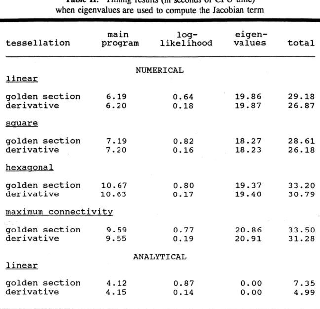
Table

II: Timing results (in seconds o f CPU time) when eigenvalues are used to compute the Jacobian term

t e s s e l l a t i o n main program lo g ­ l i k e lihoo d e i g e n ­ v a l u e s t o t a l l i n e a r

NUMERICAL

golden s e c t i o n 6 . 1 9 d e r i v a t i v e 6 . 2 0 0 . 6 4 0 . 1 8 1 9 . 8 6 1 9 . 8 7 2 9 . 1 8 2 6 . 8 7 square g olden s e c t i o n d e r i v a t i v e 7 . 1 9 7 . 2 0 0 . 8 2 0 . 1 6 1 8 . 2 7 1 8 . 2 3 2 8 . 6 1 2 6 . 1 8 hexagonal g olden s e c t i o n d e r i v a t i v e 1 0 . 67 1 0 . 63 0 . 8 0 0 . 1 7 1 9 . 3 7 1 9 . 4 0 3 3 . 2 0 3 0 . 7 9 maximum c o n n e c t i v i t y golden s e c t i o n 9 . 5 9 d e r i v a t i v e 9 . 5 5 0 . 7 7 0 . 1 9 20.86 2 0 . 9 1 3 3 . 5 0 3 1 . 2 8 l i n e a r

ANALYTICAL

golden s e c t i o n 4 . 1 2 d e r i v a t i v e 4 . 1 5 0 . 8 7 0 . 1 4

0.00

0

.

00

7 . 3 5 4 . 9 9

cases the golden section search converges in about 80 iterations. Even the maximum connectivity tessellation, an upper bound, which seemingly presents a more difficult numerical estimation problem for the derivative procedure, does not require additional golden section iterations. However, a wider range o f

p

values and data sets needs to be explore before a strong recommendation can be posited here.

A second benefit-cost trade-off pertains to the need for numerical eigenvalues. The time requirement involved here should increase exponentially as n continues to get larger. Even with the moderate tessellation sizes analyzed here, 67 percent o f computing time is being consumed by the eigenvalue computations necessary to calculate the Jacobian term. Subsequent experiments will explore, in more detail, how these timing requirements change as n increases, letting n sequentially reach 502. The linear tessellation eigenvalues presented in

Property 2

have been used to begin to benchmark that case; essentially a 75 percent reduction in CPU time is observed here when this substitution is made. Because analytical eigenvalues are not known for the remaining three cases, equation (3) will be used to evaluate them, with the same expectation concerning a reduction in CPU time. Additional information will be gleaned from a parallel set o f experiments using matrix C for the linear,

Table H I.

Estimation Statistics for the Optimization Procedures o p t im iz a t io n t e s s e l l a t i o n procedure n A P T l i n e a r g o ld e n search 42 0 . 2 7 9 0 4 - 0 .0 5 8 5 7 8 1 202 - 0 .0 4 8 7 3 - 0 .0 2 1 2 8 83 d e r i v a t i v e 42 0 . 2 7 9 0 4 - 0 .0 5 8 5 7 11 (10) 202 - 0 .0 4 8 7 3 - 0 .0 2 1 2 8 12 sq u ar e g old en search 42 0 . 2 7 2 5 3 - 0 .1 4 1 1 7 79 202 - 0 .0 4 3 4 4 - 0 .0 5 6 5 5 81 d e r i v a t i v e 42 0 . 2 7 2 5 3 - 0 .1 4 1 1 7 19 20 2 - 0 .0 4 3 4 4 - 0 .0 5 6 5 5 11 h e x a g o n a l g old e n search 42 0 . 2 7 7 9 2 - 0 .2 6 8 5 7 79 20 2 - 0 .0 4 9 1 7 - 0 .1 1 3 0 9 80 d e r i v a t i v e 42 0 . 2 7 7 9 2 - 0 .2 6 8 5 7 11 20 2 - 0 .0 4 9 1 7 - 0 .1 1 3 0 9 13 maximum g old e n search 42 0 . 3 3 4 8 6 - 0 .4 2 2 0 2 78 c o n n e c t i v i t y 2 0 2 - 0 .0 3 2 1 6 - 0 .0 5 2 0 1 82 d e r i v a t i v e 42 0 . 3 3 4 8 6 - 0 .4 2 2 0 2 19 202 - 0 .0 3 2 1 6 - 0 .0 5 2 0 1 26 N o te: f i g u r e s in p arentheses are fo r r e s u l t s o b t a in e d w it h a n a l y t i c a l e ig e n v a lu e s t h at d i f f e r from those r e s u l t s o b t a i n e d w it h numerical e i g e n v a l u e s .

square, and maximum connectivity tessellations, all o f which have known analytical eigenvalues (see Appendix A for the maximum connectivity case).

One final benefit-cost trade-off suggests that putting effort into finding at least a closed form approximation for the Jacobian term may well be more profitable than putting effort into a most efficient matrix C and/or matrix W construction. Two-to-three times as much time is consumed with eigenvalue calculations than with all o f the main program executions. Further, at least some time must be devoted to matrix construction o f some type, whereas all but a trace o f the eigenvalue calculation time can be eliminated (see Table I). 6. Concluding comments

The Jacobian term, or the normalizing factor for a spatial Gaussian process, introduces a complexity into spatial statistics and spatial econometrics estimation that tends to be distracting to researchers. Its computation is time-consuming, and can be quite problematic, since it is based upon an n-by-n matrix. Originally this term was calculated using matrix determinants. Replacement o f the determinant with its eigenvalue counterpart greatly facilitates computation. But, solving the eigenvalue problem can require considerable computer resources, too. Closed form approximations have been proposed to circumvent this problem. A very promising one is equation (3).

The preliminary timing experiment results summarized here are at least initially illuminating. As Table I results indicate, though, timing statistics are not measured without error. GPROF statistics are affected by what other software simultaneously is resident in RAM. Thus, repeated runs need to be executed, and averaged. This same point can be made with regard to using a single set o f pseudo-random numbers. Nevertheless, the results obtained here concur with previous ones (see Griffith, 1990b).

In conclusion, putting effort into removing the Jacobian term as a major computational obstacle in the implementation o f spatial statistics and spatial econometrics techniques seems to be a worthwhile endeavor, and in turn should help foster the dissemination o f these techniques.

7. Bibliography

Ahuja, N., and B. Schächter. (1983).

Pattern Models.

New York: Wiley.

Berman, A ., and R. Plemmons. (1979).

Non-negative Matrices in the Mathematical Sciences.

New York: Academic Press.

Griffith, D. (1980). "Towards a theory o f spatial statistics,"

Geographical Analysis.

Vol. 12: 325-339.

Griffith, D. (1988). "Estimating spatial autoregressive model parameters with commercial statistical packages,"

Geographical Analysis.

Vol. 20: 176-186.

Griffith, D. (1990a). "A numerical simplification for estimating parameters o f spatial autoregressive models," in

Spatial Statistics: Past, Present, and Future

, edited by D. Griffith, pp. 185-195. Ann Arbor, MI: Institute o f Mathematical Geography. Griffith, D. (1990b). "Supercomputing and spatial statistics: a reconnaissance,"

The

Professional Geographer.

Vol. 42: 481-492.

Griffith, D. (1992a). "Simplifying the normalizing factor in spatial autoregressions for irregular lattices,"

Papers in Regional Science.

Vol. 71: 71-86.

Griffith, D. (1992b). "The Jacobian approximation: a computational simplification supporting exploratory spatial data analysis," paper presented in the

Exploratory

Spatial Data Analysis

Workshop, Free University, Amsterdam, September 9-11,

1992.

Martin, R. (1992). "Approximations to the determinant in Gaussian maximum likelihood estimation o f some spatial models,"

Communications in Statistics:

Theory and

Methods.

Vol. 21: in press.

Ord, J. (1975). "Estimation methods for models o f spatial interaction,"

Journal o f the

American Statistical Association.

Vol. 70: 120-126.

Press, W ., etal. (1986).

Numerical Recipes: The Art of Scientific Computing.

Cambridge: CUP.

Ripley, B. (1990). "Gibbsian interaction models," in

Spatial Statistics: Past, Present, and

Future

, edited by D. Griffith, pp. 3-25. Ann Arbor, MI: Institute o f Mathematical Geography.

Schwenk, A ., and R. Wilson. (1978). "On the eigenvalues o f a graph," in

Selected Topics

in Graph Theory

, edited by L. Beineke and R. Wilson, pp. 307-336. London: Academic Press.

Wames, J., and B. Ripley. (1987). "Problems with likelihood estimation o f covariance functions o f spatial Gaussian processes,"

Biometrika.

Vol. 74: 640-642.

APPENDIX A

Improved approximations for and X ^ o f matrix C, the maximum connectivity case

The principle o f

The Interlacing Theorem

can be used to improve results for the binary matrix maximum connectivity case. The known analytical eigenvalues here are, from Property 6,-1 and

Xac =

Vt

= 2 cos[2 kx/(n-l)]; k = 1, 2 , ..., [n/2 j - 1 .

Because the surface partitioning involved may be represented by a graph, say G, and the two areal units linked to all others by the vertices v, and v2, then

rjk

come from the eigenvalues o f the sub-graph (G - v, - v2). The fully ordered (descending ranking) set o f eigenvalues, with the know -1 value removed and for convenience labelled X„, may be written as

Xmin ^

Vnl2-\

^ Xn_3 ^

T]

n/2-2 ^ ••• ^

^¡2

^ X3 TJj Xmax , if n is even, and

Xmin ^ Xn-2 ^ ^7[n/2]-1 ^ ^n-4 ^ ^?|n/2]-2 ^ ••• ^

V

2 ^ X3 ^ ^ Xmax , if n is odd. Further,

X2k+1 - 2 cos[(2 k + l ) 7r/(n-l)], k = 1, 2, ..., |[n/2] - 2

increasingly is a good approximation for the interlacing eigenvalues as n increases. When n is odd, Xn_2 * 2 cos[(n-2 )-7r/(n-l)]. It is a reasonable approximation for small-to-moderate n, as well. For example, where n = 25,

^

2

k + l

2cos [ ( 2k+l) 77/24 ]

^

2

k+l

2cos[ (2k+l) 7T/24 ]

1.86122

1.84776

-0.25462

-0.26105

1.59916

1.58671

-0.76058

-0.76537

1.22870

1.21752

-1.21432

-1.21752

0.77506

0.76537

-1.58492

-1.58671

0.26914

0.26105

-1.84707

-1.84776

And, X23 =

-

1

.

98281

,

versus

2

c o s

(

23

t

/

24

) = -

1

.

98289

.

This approximation allows Xmax and X ^ to be estimated, quite accurately, as well, with the following equations:

and hence Xmin = {1 + 2cos[ir/(n-l)]} - X ^ .

In the limit, these two approximations converge upon their exact counterparts. But, even for relatively small n they yield quite good estimates. For instance,

n ''m a x ^nuut ^min ^m in 8 4 . 8 8 8 2 4 . 8 3 8 5 - 2 .0 8 6 3 - 2 . 2 1 0 1 9 5 . 1 8 9 5 5 . 1 3 7 8 - 2 .3 4 1 7 - 2 . 4 5 2 1 19 7 . 3 3 5 9 7 . 2 9 6 6 - 4 .3 6 6 3 - 4 .4 1 8 0 20 7 . 5 0 6 0 7 . 4 6 8 1 - 4 .5 3 3 3 - 4 .5 8 2 5 21 7 . 6 7 1 4 7 . 6 3 4 7 - 4 .6 9 6 0 - 4 .4 7 2 9 39 1 0 . 1 1 3 2 1 0 . 0 9 1 - 7 .1 2 0 1 - 7 .1 4 5 8 40 1 0 . 2 2 8 7 1 0 . 2 0 7 - 7 .2 3 5 2 - 7 .2 6 0 3 41 1 0 . 3 4 2 6 1 0 . 3 2 1 4 - 7 .3 4 8 8 - 7 .3 7 3 3 59 1 2 . 1 8 7 2 1 2 . 1 7 1 9 - 9 .1 9 0 2 - 9 .2 0 7 3 60 1 2 . 2 8 0 4 1 2 . 2 6 5 - 9 .2 8 3 3 - 9 .3 0 0 1 61 1 2 . 3 7 2 8 1 2 . 3 5 8 0 - 9 .3 7 5 6 - 9 .3 9 2 1 79 1 3 . 9 1 8 9 1 3 . 9 0 7 - 1 0 .9 2 0 5 - 1 0 .9 3 3 80 1 3 . 9 9 9 2 1 3 . 9 8 8 - 1 1 .0 0 0 8 - 1 1 .0 1 3 81 1 4 . 0 7 8 9 1 4 . 0 6 8 - 1 1 .0 8 0 5 - 1 1 .0 9 3 99 1 5 . 4 3 6 8 1 5 . 4 2 7 - 1 2 .4 3 7 9 - 1 2 .4 4 8 100 1 5 . 5 0 8 4 1 5 . 4 9 9 - 1 2 .5 0 9 4 - 1 2 .5 2 0 101 1 5 . 5 7 9 6 1 5 . 5 7 0 - 1 2 .5 8 0 6 - 1 2 .5 9 1 199 2 1 . 3 5 5 6 2 1 . 3 5 1 - 1 8 .3 5 5 9 - 1 8 .3 6 1 200 2 1 . 4 0 5 9 2 1 . 4 0 1 - 1 8 .4 0 6 2 - 1 8 .4 1 1

When combined with the linear geographic landscape eigenfunction results, this set of estimates allows the two limiting cases to be evaluated, establishing both upper and lower bounds on the Jacobian term, without ever having to numerically extract the n eigenvalues from an n-by-n matrix.

RESUME EN FRANÇAIS

ETAPES NECESSAIRES AFIN DE RENDRE

L ’INFORMATIQUE PLUS FACILE POUR L ’ESTIM ATION DE MODELES SPATIAUX STATISTIQUES ET ECONOMETRIQUES 1. Situation

La statistique spatiale et l’économétrie spatiale cherchent à déceler l ’ information redondante qui existe dans toutes les données géographiques. Si l ’on n’ enlève pas cette information redondante, les estimateurs traditionnels des paramètres seront moins corrects. Le prix à payer à cet effect est un surplus de calcul numérique. Des experts ont fait des tentatives pour réduire cette charge d’ informatique. L ’ objectif primaire de notre communication est de procéder à une évaluation des avantages et des coûts nécessaires pour réaliser à exécution cette informatique plus facile.

Tout d’abord l ’on suppose que l ’on ait divisé une surface en une mosaïque habituelle de carrés. Il faut garder l ’arrangement bi-dimensionnel des ces éléments pour capter les renseignements sur leur localisation, et s’occuper alors de l’information redondante. On peut construire un tableau numérique, ou une matrice, qui représente cet arrangement. Le plus commun est la matrice de contiguité n-sur-n, C. Si deux éléments d’ emplacement sont côte à côte sur la surface géographique, l ’élément de la matrice (Cÿ) sera égal à 1 ; sinon à 0. On peut convertir cette matrice à une matrice W de la manière suivante: = Cÿ /E"=1 c^.

Un modèle de statistique spatiale porte le nom de modèle "autorégressif simultané" (SAR). Il exprime la valeur de la variable mesurée sur une unité spatiale comme une fonction de la somme des valeurs de cette variable autour de l’ unité spatiale, si on utilise la matrice C. On écrit la fonction log-probabilité comme suit:

ln(L)

= (-n/2)//i(2x) - (n/2)/n(o2) - (l/2)/«[det(I -

pC)2]

-(Y - X0)‘(I

- pCyÇL -

pC )(Y - XJ8)/(2o2) (1) [voir l ’équation (1) de la communication].

Cette fonction de densité de probabilité est la même que la fonction multivariée normale de densité avec une observation et n variables.

Dans l ’équation (1) est l ’ équation de régression ordinaire. Elle donne le modèle SAR, qu’on écrit pour l ’estimer selon l’équation (2):

Y/J(p) = [pCY +

Xp -

pCX/3]/J(p) + £/J(p) . (2) [voir l ’équation (2) de la communication].

J(p) 2 = {/«[det(I - p C )]} 2/n est le Jacobien de l’équation (2). 2. Sources de l ’importance des calculs

La statistique spatiale est très intensive en calcul numérique. Cette intensité de calcul trouve son origine dans trois sources principales; chacun d’elles est présenté dans l ’équation (2). Tout d’abord, la construction de la matrice C est fastidieuse et elle peut prendre beaucoup de temps. Ensuite vient la construction des variables suivantes, spatialement décalées: C Y, CXj, et C£. Enfin, il faut calculer le Jacobien, J(p), qui se trouve au dénominateur cependant que le paramètre d’autocorrélation spatiale, p, se trouve au numérateur, ce qui appelle une solution NLS. Ripley (1990) soutient que ce Jacobien introduit les complications d’estimation qui ont poussé les chercheurs spatiaux à éviter l’ emploi de techniques spatiales de statistique et d’économetrie.

Si n’on connaît pas p, la NLS connaîtra un grand nombre d’itérations pour son estimation. On peut utiliser, soit les dérivées analytiques, soit une démarche de recherche, dans le cours de ces itérations. Wames et Ripley (1987) déconseillent l ’ utilisation des dérivées parce que la surface de la fonction de probabilité sériât trop chaotique; de plus, les dérivées sont aussi trop désordonnées. On peut trouver une solution pour l ’équation (2) en prenant un échantillon systématique des valeurs de p dans l ’espace faisable du paramètre, donc en calculant une solution OLS pour chacune des ces valeurs. La solution NLS est la solution OLS avec la plus petite des MSEs. Puisque chacune des itérations nécessite le calcul d’ une régression OLS différente, et qu’il faut réévaluer le Jacobien pour chacune de ces itérations, peut d’ intensité de calcul numérique est évidente. Notre communication évalue les avantages et les coûts d’ une simplification du Jacobien, afin de rendre le calcul moins lourd.

3. Une brève histoire du Jacobien

Quand Whittle (1954) faisait les estimations du modèle spatial SAR, il utilisait une approximation du Jacobien. Cette approximation venait de la comparaison du passage de la limite de -/n[det(I - pC)]/n à l’intégrale du logarithme de la densité spectrale pour un processus immobile fonctionnant partout dans la mosaïque habituelle de carrés des éléments spatiaux. A mesure que les ordinateurs sont devenus plus puissants, cette approximation est devenue moins utile, cela seulement parce que la plupart de bases des données géographiques sont contenues dans n < 100. Les données satellites et les SIG ont changé cette situation, concentrant une fois de plus l ’attention sur le Jacobien.

Il y a trois raisons de vouloir estimer le Jacobien. Tout d’abord, le calcul du detérminant d’ une grande matrice demande des ressources considérables d’ ordinateur, ou est

même impossible; de plus il serait inexact numériquement. Ensuite, le calcul fréquent du logarithme de ce detérminant dans chaque itération NLS sera lent, et utilisera trop de ressources d’ordinateur. Finalement, le fait qui les chercheurs spatiaux soient libérés des calculs difficiles et pénibles accompagnant la statistique et l’économetre spatiales permettra (1) l ’ usage de logiciels commerciaux ordinaires, et (2) un effort plus grand consacré aux aspects substantifs des problèmes de recherche.

3.1. Calcul du detérminant de l ’inverse de la matrice de covariance

On peut calculer le detérminant de la matrice (I - pW ) de fason normale selon l’algèbre des matrices

(voir le texte de la communication).

Manipuler les lignes et les colonnes consomme plus de temps d’ ordinateur; obtenir une expression simple, comme (1 - p2) dans l ’exemple, est plus rapide.

Peut-être le premier par dans cette direction est venue en substituant

n?=1(l

-

p \ )

à

t(I - pW), où Xj sont les n valeurs propres de la matrice W.

3.2. Remplacement du detérminant de la matrice par sa double valeur propre

Ord (1975) a popularisé l ’ utilisation d’ un résultat bien connu de l ’ algèbre des matrices. En conséquence, le Jacobien du modèle SAR devient:

J(p)2 = - 2E£=1

ln(

1 - pX^/n .

Il faut maintenant calculer n valeurs propres; mais à chaque itération l ’ on recalcule seulement la somme des n logarithmes.

Une solution meilleure serait d’avoir les expressions analytiques des valeurs propres nécessaires.

3.3. Résultats de la recherche des valeurs propres analytiques

Les tentatives pour trouver les expressions analytiques des valeurs propres ont été seulement une réussite partielle. Les trois propriétés suivantes sont bien connues:

Propriété 1

: pour une matrice C représentant une surface linéaire, les valeurs propres de la matrice sont

Xk = {2cos[k7r/(n+l)]; k = 1, 2, ..., n} .

Propriété 2:

pour une matrice W représentant une surface linéaire, les valeurs propres de la matrice sont

Xk = {cos[kn7(n-l)]; k = 0, 1, ..., n-1} .

Propriété 3

: pour une matrice C représentant une surface rectangulaire P-sur- Q, qu’ on a divisée en une mosaïque habituelle de carrés, les valeurs propres de la matrice sont

Xpq = {2cos[pir/(P+l)] + 2cos[q7r/(Q+l)]; p = 1, 2, . . . , P & q = 1,2, . . . , Q } .

Propriété 3 est extrêmement utile pour des analyses statistiques spatiales de données satellites. Mais la plupart des surfaces dans un SIG ne sont pas une mosaïque habituelle des figures géométriques. En ce moment il n’ y a pas d’équivalent de la propriété 3 pour une matrice W. De cette façon, nous avons trouvé la propriété partielle suivante, à l ’ occasion de nos recherches, et que nous présentons ici:

Propriété 4:

pour une matrice W représentant une surface carrée P-sur-P qu’ on a divisée en une mosaïque habituelle de carrés, P des valeurs propres sont zéro, et P des valeurs propres sont égales à

Xk = {cos[kx/(P-l)]; k = 0, 1, P- l } . Le reste sont des paires doubles de forme ± X h.

La United States Environmental Protection Agency (USEPA) a divisée les Etats-Unis en une mosaïque habituelle d’ hexagones. Une propriété partielle sur cette géométrie est la suivante:

Propriété 5:

la plus grande valeur propre pour la matrice C représentant un surface rectangulaire P-sur-Q, qu’on a divisée en une mosaïque habituelle d’ hexagones, où P est la dimension "nord-sud" et Q est la dimension "est- ouest," se trouve dans l ’intervalle

(19.80837 - 19.57972X0 - 20.40408XP + 18XPC»

1 - 2XP - 2xQ + 3XPQ _ A»« _ 0 ,

P & Q > 5.

En ce moment, la seule propriété que nous connaissions pour la matrice W , est le résultat ordinaire comme quoi la plus grande valeur propre est égal à 1.

Enfin, presque toutes les surfaces des SIGs ne présentent pas sur les mosaïques habituelle des figures; seule une limite supérieure est disponible ici. La situation plane du plus grand nombre de connexions a la propriété partielle suivante:

Propriété 6:

pour une matrice C représentant une surface avec le plus grand nombre de connexions, une liste des valeurs propres inclut -1 et

Xk = {2cos[2kx/(n-l)]; k = 1, 2, ..., [n/2j - 1 } ,

(voir le texte de la communication). Plus grande valeur propre se trouve dans l ’intervalle

[5n + 4(n - 4 + V 3 )/ (n - 1) + 4/3 - 21]/[3(n - 2)] < Xmax < 1 + (2/3 - 6)A/(n - 1) + 2/(n - 1) .

On peut estimer d’autres valeurs propres inconnues avec précision (voir l ’ annexe A de la communication).

Ajoutons encore le,

Propriété

7: pour une matrice W représentant une surface avec un plus grand nombre de connexions, une liste des valeurs propres inclut 1, -l/(n-l), et -1/2 (voir le texte de la communication).

En conclusion, l ’on peut dire que les résultats obtenuis jusqu’à present sont loin d’être complets.

3.4. Approximations utiles du Jacobien.

La meilleure approximation du Jacobien serait une expression exacte, que éviterait d’avoir besoin de calculer les valeurs propres. Malheureusement, en ce moment la seule expression exacte existe pour une surface linéaire. Il s’agit, pour le modèle SAR avec matrice C, de

J(p) = [(n + l)/n]/n(2) +

ln(

1 - 4p2)/(2n) -

ln{[

1

+ V ( l

- 4p2)]n+1 - [1

- V ( l -

4p2)]n+,}/n ,

et avec matrice W ,

J(p) = [(n - l)/n]/n(2) -

ln{

1 - p2)/(2n) -

ln{[l + V ( \

- p2) ] " 1 - [1

- V ( l

- p2)]n,}/n

Une deuxième approche consister dans le développement d’ une approximation presque égale au Jacobien. Martin (1992) propose d’employer le premier des termes en écrivant

ln

[(I - pC)'1/n] comme un série (voir le texte de la communication). Un problème avec cette approximation est qu’elle requiert le calcul des puissance d’ une matrice n-sur-n. Griffith (1990a, 1992a) propose d’employer l’équation (3), qu’ il faut estimer. L ’ équation (3) est préférable à la méthode de Martin. Mais l’ utiliser demande un tableau des valeurs pour a, „,

Yl,n> ®2,n> T2,n*

4. Quelques résultats de mesures du temps de calcul

Nous avons lancé des expériences de chronomètre du temps nécessaire pour explorer le problème du Jacobien. Nous conduirsons ces expériences avec un ordinateur IBM RISC/System 6000. Cette machine utilise le système opératoire A IX Unix. Nous emploions le logiciel GPROF afin d’obtenir la statistique du temps de calcul, et nous emploions la bibliothèque IBM ESSL afin de calculer les detérminants des matrices et les valeurs propres. Touts les calculs se font en double précision. Nous écrivons notre programme en FORTRAN77.

Le premier résultat des ces expériences sont repris aux tableaux I et II (voir le texte de la communication); un résumé en est suivant:

(a) 20-30 % du temps de calcul et pris par le programme

main,

qui construit les matrices C et W , et la matrice symmetrique pour W;

(b) la sous-routine "golden search" utilise approximativement 10% plus de temps que la sous-routine "derivative," à cause du surplus d’itérations;

(c) approximativement 2/3 du temps de calcul est consacré aux valeurs propres;

(e) on peut élimines tout de temps de calcul des valeurs propres numériques, en utilisant une fonction appropriée.

Une comparaison des précision obtenues se trouve au tableau III (voir le texte de la communication); un résumé en est le suivant:

(a) il n’ y a pas différences visibles entre les deux sous-routines;

(b) la sous-routine "golden search" utilise approximativement le même nombre d’itérations pour toutes les surfaces;

(c) la sous-routine "derivative" utilise plus d’itérations pour la surface avec le plus grand nombre des connexions; et,

(d) il y a une différence sensible l’ utilisation des valeurs propres numériques et celle des valeurs propres analytiques.

5. Avantages et coûts décelés

Tout d’ abord, la méthode "golden section search" demande plus de temps, mais serait plus fiable que la méthode "derivative." Le temps de calcul supplémentaire n’est pas excessif.

Ensuite, le calcul des valeurs propres numériques utilise une majeure partie du temps ordinateur. Il faut connaître ces valeurs propres afin de pouvoir calculer le Jacobien. Un’effort en vue de trouver, soit des expressions pour calculer les valeurs propres analytiques, soit des approximations du Jacobien, éliminera cette exigence de temps de calcul.

Finalement, on gagnera moins de la trouvaille d’ une méthode plus efficace pour construire les matrices C et W , que pour résoudre le problème du Jacobien.