HAL Id: hal-00328591
https://hal.archives-ouvertes.fr/hal-00328591
Submitted on 17 Jun 2003
HAL is a multi-disciplinary open access
archive for the deposit and dissemination of
sci-entific research documents, whether they are
pub-lished or not. The documents may come from
teaching and research institutions in France or
abroad, or from public or private research centers.
L’archive ouverte pluridisciplinaire HAL, est
destinée au dépôt et à la diffusion de documents
scientifiques de niveau recherche, publiés ou non,
émanant des établissements d’enseignement et de
recherche français ou étrangers, des laboratoires
publics ou privés.
The potential of ground gravity measurements to
validate GRACE data
D. Crossley, J. Hinderer, M. Llubes, Nicolas Florsch
To cite this version:
D. Crossley, J. Hinderer, M. Llubes, Nicolas Florsch. The potential of ground gravity measurements
to validate GRACE data. Advances in Geosciences, European Geosciences Union, 2003, 1, pp.71.
�hal-00328591�
Geosciences
The potential of ground gravity measurements to validate GRACE
data
D. Crossley1, J. Hinderer2, M. Llubes3, and N. Florsch4
1Earth and Atmospheric Sciences, Saint Louis University, 3507 Laclede Ave., St. Louis, MO 63103, USA 2Institut de Physique du Globe / EOST, 5 Rue Descartes, Strasbourg 67084, France
3LEGOS/CMES/CNRS Toulouse, France
4Department de Geophysique Appliquee, UMR 7619 Sisyphe, Paris, France
Abstract. New satellite missions are returning high
pre-cision, time-varying, satellite measurements of the Earth’s gravity field. The GRACE mission is now in its calibration/-validation phase and first results of the gravity field solu-tions are imminent. We consider here the possibility of exter-nal validation using data from the superconducting gravime-ters in the European sub-array of the Global Geodynam-ics Project (GGP) as ‘ground truth’ for comparison with GRACE. This is a pilot study in which we use 14 months of 1-hour data from the beginning of GGP (1 July 1997) to 30 August 1998, when the Potsdam instrument was relocated to South Africa. There are 7 stations clustered in west central Europe, and one station, Metsahovi in Finland. We remove local tides, polar motion, local and global air pressure, and instrument drift and then decimate to 6-hour samples. We see large variations in the time series of 5–10 µgal between even some neighboring stations, but there are also common features that correlate well over the 427-day period. The 8 stations are used to interpolate a minimum curvature (grid-ded) surface that extends over the geographical region. This surface shows time and spatial coherency at the level of 2– 4 µgal over the first half of the data and 1–2 µgal over the lat-ter half. The mean value of the surface clearly shows a rise in European gravity of about 3 µgal over the first 150 days and a fairly constant value for the rest of the data. The accuracy of this mean is estimated at 1 µgal, which compares favor-ably with GRACE predictions for wavelengths of 500 km or less. Preliminary studies of hydrology loading over Western Europe shows the difficulty of correlating the local hydrol-ogy, which can be highly variable, with large-scale gravity variations.
Key words. GRACE, satellite gravity, superconducting
gravimeter, GGP, ground truth
Correspondence to: D. Crossley ([email protected])
1 Introduction
The stimulus for this study originated with Wahr et al. (1998) who discussed the expected accuracy of surface gravity fluc-tuations for the proposed GRACE mission. They demon-strated that a careful accounting for the various contribu-tions to time varying gravity would permit the determina-tion of small time-varying signals such as variadetermina-tions in con-tinental water storage. It was immediately clear that we should consider the possibility of combining satellite data and ground-based data from the Global Geodynamics Project (GGP; Crossley et al., 1999). The GGP superconducting gravimeter (SG) network is far too sparse geographically to be suitable as a global gravity field, but there are sub-arrays of instruments, particularly in Asia and Europe, that war-rant closer consideration. Preliminary attempts at producing a ground-based map of gravity variations were reported by Crossley and Hinderer (1999) and later by Crossley and Hin-derer (2002).
Recently, Velicogna and Wahr (2001) suggested that ground based gravity measurements cannot usefully con-tribute to the validation or analysis of GRACE data. They argue that the radius over which a single ground-based mea-surement extends (several 10’s km) is incompatible with the wavelengths of satellite-derived fields (> 200 km). Second, using GGP data from the International Centre for Earth Tides, they used statistical arguments to argue against any correlation of the signals over long time spans. The wave-length argument is true for a single station but the limitation can be overcome, to some extent, by the use of a gravity ar-ray. The question of the treatment of GGP data can only be answered by taking care in the analysis to preserve long-term integrity of each data set. Here we address both issues by processing the GGP data for a specific epoch, finding that the correlation between gravity variations over distances of several hundred km and time spans of several months is quite convincing.
66 D. Crossley et al.: Potential of ground gravity measurements to validate GRACE data
Table 1. European GGP stations used in the analysis
Station Code Country Instrument Latitude Longitude
Brussels BE Belgium T003 50.7986 4.3581 Membach MB Belgium C021 50.6093 6.0066 Medicina MC Italy C023 44.5219 24.3958 Metsahovi ME Finland T020 60.2172 24.3958 Potsdam PO Germany T018 52.3806 13.0682 Strasbourg ST France C026 48.6217 7.6838 Vienna VI Austria C025 48.2493 16.3579 Wettzell WE Germany SG103 49.1440 12.8780
Fig. 1. Hydrology recovery from GRACE.
2 GRACE goals
GRACE (Gravity Recovery and Climate Experiment) is a joint venture of NASA (USA), DLR (Germany), UTCSR (Texas), and GFZ (Potsdam). The mission has now been actively collecting data for about 9 months and the first re-sults are to be reported soon (AGU Abstracts, Fall Meeting 2002). The high accuracy anticipated of GRACE data should enable subtle time variations in the gravity field to be found, i.e. changes in continental water storage, the variability of ocean bottom pressure, and the redistribution of snow and ice. These changes will be determined by successive spher-ical harmonic solutions of the data with a limiting ground resolution of 100–200 km and intervals of 2–4 weeks.
The methodology follows the sequence (Wahr et al., 1998):
– assume a density change 1ρ in a layer of thickness H
(10–15 km) surrounding the Earth’s surface (i.e. the lower atmosphere and upper hydrosphere).
– convert 1ρ to a surface density distribution 1σ by
in-tegrating over H .
– expand 1σ in spherical harmonics, with coefficients
( ˆClm, ˆSlm)
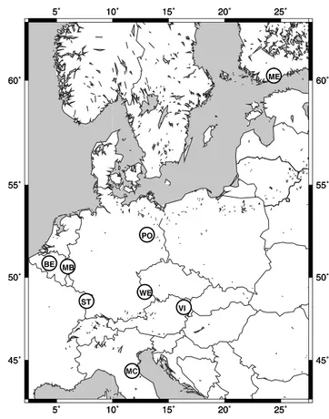
Fig. 2. GGP stations July 1997 – August 1998.
– relate these harmonics to the harmonics ( ˆClm, ˆSlm) of the gravity field, determined from the GRACE satellite orbit data, approximately every 14 days.
– deduce 1σ from ( ˆClm, ˆSlm), and thus infer 1ρ by as-suming H .
Note that 1σ does not distinguish between water, ice, or snow. It is also evident that the GRACE data will be time-aliased if there is any unmodeled variation of gravity on time scales less than 2 weeks, as seems probable for the atmo-sphere and oceans (e.g. Flechtner et al., 2002).
One of the examples considered by Wahr et al. (1998) is for Manaus, Brazil, in the Amazon River Basin (Fig. 1). The upper curve shows the predicted hydrology signal, the middle curve is the expected errors in GRACE data with all sources of modeling (PGR is post glacial rebound), and the lower trace is for GRACE errors alone. The accuracy of the recov-ery using the full 5 years of data is 2 mm of water at length scales longer than 400 km; a more recent estimate indicates better than 1 cm at 200 km or longer (Swenson et al., 2002). The errors at shorter wavelengths rise rapidly, becoming ex-cessive at wavelengths less than 200 km. The shaded box is the region where GRACE errors and GGP network errors are expected to overlap. To be competitive, ground-based gravity measurements need (a) to cover wavelengths between 100 and 1000 km and (b) to reach accuracies of less than 0.4 µgal at wavelengths between 200 and 300 km. If both conditions are satisfied, we may claim that ground-based (in
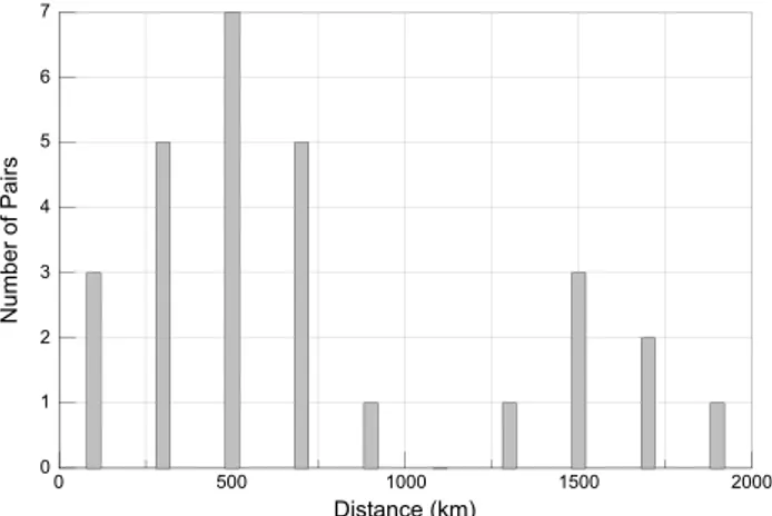
0 500 1000 1500 2000 Distance (km) 0 1 2 3 4 5 6 7 N u m b e r o f P a ir s
Fig. 3. Station distribution by pairs.
this case GGP) gravity can be used to ‘validate’ satellite mea-surements.
3 GGP data
The stations used in this study are shown in Table 1 and Fig. 2. All stations except ME are in the middle of the West-ern European landmass. The time period of this analysis was chosen to begin at the start of GGP (97/7/1) and continue to the end of the recording at PO (98/8/31). The PO SG was then reconstructed as a dual sphere instrument and moved to South Africa (Neumeyer et al., 2001). Station MC is not officially a GGP station, but data are available for this study through the work of Zerbini et al. (2001). Station BE stopped recording in 2000 and the instrument at Wettzell, which was a prototype compact dewar model (designation SG103) with unusually large drift (Harnisch et al., 2000), has been re-placed with a new dual sphere model. Also a new station, Moxa, was started in 2000 (Kroner et al., 2001). The distri-bution, or spacing, of the 8 stations taken in pairs, is plotted as a histogram in Fig. 3. The distance range of 200–1000 km is well covered, but the inclusion of a single distant station (ME) extends the coverage up to 2000 km.
4 Processing
The first step is to remove a modeled tide from each station using local tidal gravimetric factors (δ, κ) obtained from in-dependent analyses of data from each station. We include all waves with periods up to a month. For semi-annual and longer periods we use nominal elastic gravimetric values of (1.16, 0) to avoid fitting artificially the residual annual sig-nals. We also remove the effect of local atmospheric pres-sure using a nominal admittance of −0.3 µgal mbar−1; using slightly different values will not be a major source of error in the final result. The residual series are displayed in Fig. 4. It is clear station WE has a large negative drift that appears
BE 1 min -12 -8 -4 -0 m ic ro ga l 4 8 MB 1 min -2 -0 1 m ic ro ga l 3 4 ME 1 min -7 -4 -1 3 m ic ro ga l 6 9 -3 MC 1 hour -11 -8 -5 -2 m ic ro ga l 2 5 PO 1 min -4 -3 -1 -0 m ic ro ga l 1 3 ST 1 min -4 -2 -1 1 m ic ro ga l 2 4 VI 1 min -5 -3 -2 -1 m ic ro ga l 1 2 WE 1 min 0 43 85 128 171 213 day 256 299 342 384 427 -147 -88 -28 31 m ic ro ga l 90 149
Fig. 4. Gravity residuals after removal of tides, local pressure and polar motion. Note the different scales of each data set.
linear. IERS-derived polar motion was also subtracted from each data set.
5 Instrument drift
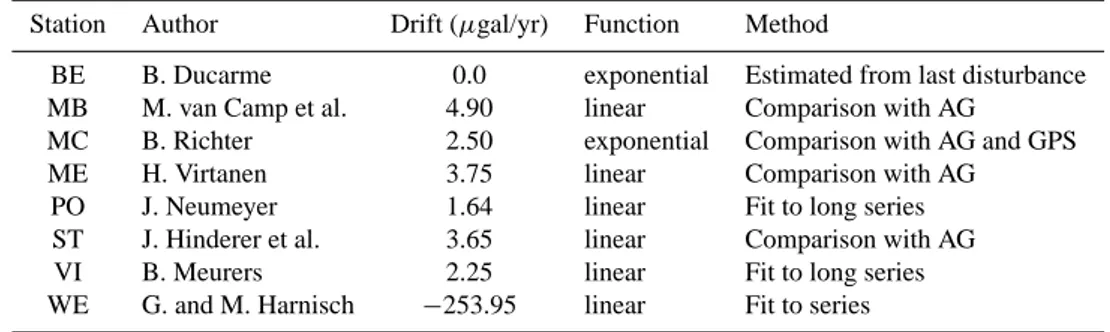
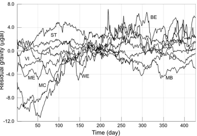
For WE, we fit simultaneously a linear drift function and a series of offsets (already corrected in Fig. 4) at fixed time lo-cations; this is done iteratively to arrive at an appropriate cor-recting function. In Fig. 5 the residuals are now plotted on a common axis, with the drift of station WE removed. We now remove the instrument drift at the other stations. Rather than do the analysis solely on the basis of the 14 months of data at our disposal, we requested assistance from the station op-erators who have analyzed their data over much longer time periods. The results are shown in Table 2. It is seen that apart from WE (discussed above), most of the stations have drift rates in the 1–4 µgal yr−1range. The most reliable estimates come from comparisons with Absolute Gravimeter data, but at some stations this was not possible. At one station (MC), the data were further checked using a series of GPS measure-ments (Zerbini et al., 2001) to establish vertical motion. The drift of station MB is a high compared to the other stations,
68 D. Crossley et al.: Potential of ground gravity measurements to validate GRACE data
Table 2. Drift functions removed for each station
Station Author Drift (µgal/yr) Function Method
BE B. Ducarme 0.0 exponential Estimated from last disturbance
MB M. van Camp et al. 4.90 linear Comparison with AG
MC B. Richter 2.50 exponential Comparison with AG and GPS
ME H. Virtanen 3.75 linear Comparison with AG
PO J. Neumeyer 1.64 linear Fit to long series
ST J. Hinderer et al. 3.65 linear Comparison with AG
VI B. Meurers 2.25 linear Fit to long series
WE G. and M. Harnisch −253.95 linear Fit to series
Fig. 5. Gravity residuals, 1 hour, mean values removed.
but it has been carefully checked and has found to be reliable (van Camp et al., 2002).
6 Global pressure loading
We now correct for the non-local atmospheric pressure ef-fects, first decimating the data further to 6-hour samples. The global atmospheric loading has been calculated by Jean Paul Boy (personal communication) using the method described in Boy et al. (2001). The assumption is that the vertical col-umn is hydrostatic and so the mass attraction and loading are dependent only on the surface pressure, here obtained from the ECMWF.
The results for the 8 stations are shown in Fig. 6 as the difference between local and global loading. The differences between global and local corrections are significant (−1.5 to +2 µgal) over short periods, but there is little or no long term trend. More importantly, all stations respond in a sim-ilar fashion, indicating that the global loading is intergrating over atmospheric masses of the same size or larger than this station distribution.
To illustrate the effect of the global loading on the grav-ity residuals, we show the results for ME, where the differ-ences are the largest (Fig. 7, in which the dashed line is the
Fig. 6. Global vs local atmospheric pressure loading.
50 100 150 200 250 300 350 400 Time (day) -6.0 -4.0 -2.0 0.0 2.0 4.0 6.0 G ra v it y re s id u a l (m g a l)
Fig. 7. Effect of global pressure loading at station ME.
local correction). Clearly the inclusion of global pressure does not significantly affect the trend of the gravity residu-als. This type of computation has since been updated (Boy and Chao, 2002) by using a three-dimensional atmospheric model and they find that seasonal changes due to global load-ing are more significant than those shown here. Their method will be incorporated in future work on this project.
ME VI PO ST MB 50 100 150 200 250 300 350 400 Time (day) -12.0 -8.0 -4.0 0.0 4.0 8.0 R e s id u a l g ra v it y (m g a l) BE WE MC
Fig. 8. Final residual gravity after all corrections.
drift in Table 2 and the atmospheric loading in Fig. 6. It can be seen the the series are somewhat flatter than Fig. 5, but still with a significant spread of values, especially during the first 150 days.
7 Spatial averaging
We need to consider how to spatially average the individ-ual station residindivid-uals to simulate the integrating effect of the satellite measurements. To estimate the spherical harmonic coefficients of a global model from such a limited amount of ground data would definitely yield poor coefficients, so we proceed differently.
We first of all fit a minimum curvature surface to the data points on which Fig. 8 is derived. This fit is performed for each 6-hour sample of the field, and one of the properties of the surface is that it goes through each of the original points. This is therefore a good interpolation procedure and we can produce contour maps of the surface as a function of time. These maps do not do any spatial averaging of the field and neighboring stations with conflicting series (e.g. BE and MB) still show up as inconsistencies (we cannot shows these maps here due to lack of space). As a second step we there-fore fit a polynomial surface to the data using the whole of this interpolated surface (not just the original data points), in order to get a robust least squares solution. We choose a third degree polynomial because this gives a reasonable smooth-ing about a wavelength of 500 km. Higher order polynomials may also be justified, but we have not investigated all possi-bilities. The resulting surface is then re-sampled at each of the original station locations and a set of smoothed time se-ries is produced (Fig. 9). The sese-ries now show much less deviation and the data that stands out from the rest is ME, due partly to its distance from the other stations and the poor control due to the lack of neighboring stations.
We now re-sample the residuals to 14 days to represent satellite repeat determinations of the field, to produce the se-ries in Fig. 10. We claim that this figure represents our
inter-ME BE MC PO 0 50 100 150 200 250 300 350 400 Time (day) -8.0 -6.0 -4.0 -2.0 0.0 2.0 4.0 6.0 8.0 S m o o th e d re s id u a ls (m g a l)
Fig. 9. Spatially smoothed residuals, 6-hour sampling.
ME PO BE MC 50 100 150 200 250 300 350 400 Time (day) -6.0 -4.0 -2.0 0.0 2.0 4.0 6.0 S m o o th e d re s id u a ls (m g a l)
Fig. 10. Spatially smoothed residuals, 14-day sampling.
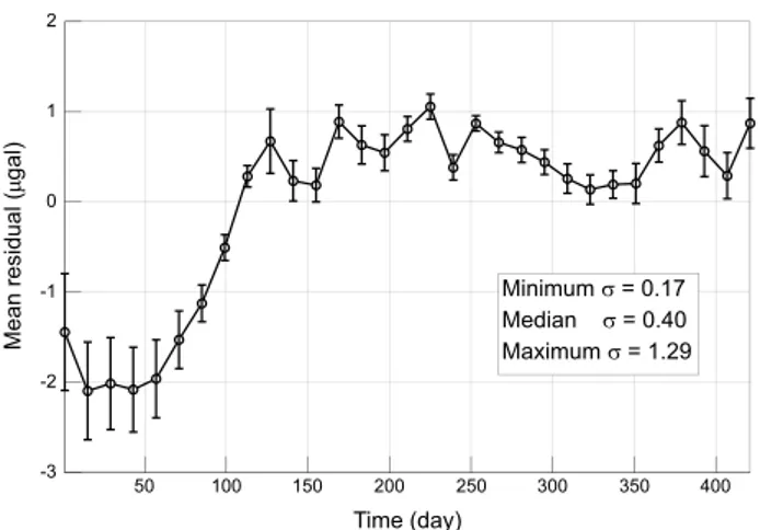
pretation of a time and space averaged picture of the gravity field. It is difficult to place error estimates on these series due to the various processing steps involved, but one further step might be to average all the series together (except ME since this is an outlying station) and compute the errors in this final average. This is done in Fig. 11, which is our final result. It shows that the 1 σ errors are of the order of 1–2 µgal for the first 150 days, and less than 1 µgal for the reset of the time period.
8 Hydrology
So far we have made no allowance for hydrology, either large scale or local, because in fact this signal will also be seen by the satellite. The variability of continental water storage is a prime target for GRACE and clearly one that affects surface gravity measurements. Van Dam et al. (2001) showed that at the GGP stations their models predict large variations of water-induced gravity changes that are frequently dominated by annual variations of the order of 10 µgal. Such effects are
70 D. Crossley et al.: Potential of ground gravity measurements to validate GRACE data 50 100 150 200 250 300 350 400 Time (day) -3 -2 -1 0 1 2 M e a n re s id u a l (m g a l) Minimum s = 0.17 Median s = 0.40 Maximum s = 1.29
Fig. 11. Evolution of the mean field, ME omitted.
difficult to separate from other possible annual signals in the residuals, e.g. global pressure effects.
At the same time the analysis of local hydrology is of-ten usefully done to remove a water signal in gravity record-ings, e.g. Crossley et al. (1998), Kroner (2001), and Virtanen (2001). Frequently there is a high correlation between local measures, such as rainfall and water table depth, and resid-ual gravity and this correlation is used to justify the mod-eling. One source of uncertainty is the interpretation of the resulting admittance, as this depends on the local porosity. Frequently the empirical estimate of porosity obtained from the admittance is difficult to verify on physical grounds.
A long-term project has been initiated to estimate con-tinental water storage in central Europe. We (Florsch and Llubes, 2002) have performed loading estimates of large-scale (2000 × 3000 km) hydrology over Europe by placing a 1 m water load on the continental crust. The vertical crustal displacement reaches a maximum of 4.6 cm at the center of the load and less than 1.0 cm outside the area. This gives a central effect of 14 µgal in gravity to which must be added about 42 µgal in direct Newtonian attraction; the total effect is therefore 0.56 µgal per cm water (at 100% porosity). At a smaller scale we have simulated a loading of 1 m water over the Alsace region of the lower Rhine Graben (about 20 × 300 km) and find a very localized loading effect of 1.6 µgal, with again the dominating direct effect of 42 µgal, thus a total of 0.44 µgal per cm water.
As is widely recognized, hydrology can be extremely
complex at regional scales. A good example can be
found at the website (http://aesn.brgm.fr/bulletin/nappes. html) run by l’Agence de L’Eau Seine-Normandie, in which the water table has been monitored at over 60 sites over
the Seine Basin since 1975. The correlation between
neighboring sites is often poor because of the geological variability, (http://aesn.brgm.fr/bulletin13/images/situation nappe.gif), whereas some sites are well correlated even at relatively large distances. Determining the true hydrological signal will inevitably require a combination of direct water table measurements and gravity observations, the latter
in-cluding both ground-based and satellite data.
9 Discussion and conclusions
One may, with some justification, question the somewhat ad-hoc procedure used to get from the gravity residuals (Fig. 8) to the smoothed integrated curve of the gravity field evolu-tion (Figs. 9 to 11). At the present time we are considering alternative ways of doing this. Nevertheless, it is evident that even in Fig. 8. there is spatial and temporal coherency of the field over the 427 days, and this becomes more obvious in the smoothed product, Figs. 9 and 10. Station ME is unusual in more than its geographic isolation from the other stations. As Virtanen et al. (2002) have shown, the loading effects of the Baltic Sea are quite strong and account for much of the variability seen in Fig. 10. So far this loading has not been corrected in the current study, but it will be seen by a satel-lite, so one has to be careful to compare fields that have been consistently processed.
Further work is being done to extend these series to more recent years, in particular into 2000 when the CHAMP satel-lite started to produce results. It is difficult to produce a grav-ity surface in real time from GGP data due to the care needed in processing and the need to make systematic absolute grav-ity measurements to check the drift. Nevertheless the GGP data certainly enables such maps of the evolution of the Eu-ropean gravity field to be made. A longer-term goal might be to establish further SGs in the missing regions (e.g. Spain, Poland, Northern Germany) that would undoubtedly signifi-cantly improve the quality of the gravity field estimation. In future we believe this work will provide a useful source of data with which GRACE and other satellite missions may be compared.
Acknowledgements. We thank the various European SG station
op-erators (Table 2) for making the data available through GGP. This research was supported by CNRS; it is EOST contribution No. 2002-16-7516.
References
Boy, J.-P., Gegout, P., and Hinderer, J.: Reduction of surface grav-ity data from global atmospheric loading, Geophys. J. Int., 149, 534–545, 2000.
Boy, J.-P. and Chao, B. F.: Effects of the vertical structure of the atmosphere on gravity at satellite altitude, Geophys. Res. Abs., EGS 27 General Assembly, 4, EGS02-A-03837, 2002.
Crossley D., Xu, S., and van Dam, T.: Comprehensive analysis of 2 years of data from Table Mountain, Colorado, Proc. 13th Int. Symp. Earth Tides, Brussels, July 1997, Royal Observatory of Brussels, 659–668, 1998.
Crossley, D. J. and Hinderer, J.: Global gravity campaigns – from the ground (GGP) to the sky (GRACE), IUGG XXII General As-sembly, Abstract Volume A, 71–72, 1999.
Crossley, D. J., Hinderer, J., Casula, G., Francis, O., Hsu, H.-T., Imanishi, Y., Meurers, B., Neumeyer, J., Richter, B., Shibuya, K., Sato, T., and van Dam, T.: Network of superconducting gravime-ters benefits several disciplines, EOS, 80, 121–126, 1999.
Crossley, D. and Hinderer, J.: GGP Ground Truth for Satellite Gravity Missions, Bull. D’Inf. Marees Terr., 136, 10 735–10 742, 2002.
Flechtner, F., Zlotnicki, V., and Pekker, T.: Atmospheric and oceanic gravity field de-aliasing for GRACE, Geophys. Res. Abs., EGS 27 General Assembly, 4, EGS02-A-01557, 2002. Florsch, N. and Llubes, M.: Geodetic impact of acquifer on regional
gravity survey, Geophys. Res. Abs., EGS 27 General Assembly, 4, EGS02-A-05536, 2002.
Harnish, M., Harnisch, G., Jurczyk, H., and Wilmes, H.: 889 days of registrations with the superconducting gravimeter SG103 at Wettzell (Germany), Cahiers du Centre Europeean de Geody-namique et de Seismologie, 17, 25–37, 2000.
Kroner, C.: Hydrological effects on Gravity at the Geodynamic Ob-servatory, Moxa. J. Geod. Soc Japan, 47 (1), 353–358, 2001. Kroner, C., Jahr, T., and Jentzsch, G.: Comparison of Data Sets Recorded with the Dual Sphere SuperconductingGravimeter CD 034 at the Geodynamic Observatory, Moxa. J. Geod. Soc Japan, 47 (1), 398–403, 2001.
Neumeyer, J., Brinton, E., Fourie, P., Dittfeld, H.-J., Pflug, H., and Ritschel, B.: Installation and First Data Analysis of the Dual Sphere Superconducting Gravimeter at the South African Geo-dynamic Observatory, Sutherland, J. Geod. Soc. Japan, 47 (1), 316–321, 2001.
Swenson, S., Wahr, J., and Milly, P. C. D.: Large-scale hydrology inferred from GRACE estimates of time-variable gravity,
Geo-phys. Res. Abs., EGS 27 General Assembly, 4, EGS02-A-03671, 2002.
Van Camp, M., Warnant, R., and Francis, O.: Crustal deformations in Membach, Belgium, Geophys. Res. Abs., EGS 27 General As-sembly, 4, EGS02-A-00860, 2002.
Van Dam, T., Wahr, J. M., Milly, P. C. D., and Francis, O.: Gravity changes due to continental water storage, J. Geod. Soc. Japan, 47 (1), 249–254, 2001.
Velicogna, I. and Wahr, J.: Potential problems with the use of gravimeter data for GRACE Cal/Val., EOS Trans. AGU, 82 (47), Fall Meet. Suppl., Abstract G51A-0242, 2001.
Virtanen, H.: Hydrological studies at the Gravity Station Metsahovi in Finland, J. Geod. Soc. Japan, 47 (1), 328–333, 2001. Virtanen, H., Makinen, J., Bilker, M., Poutanen, M., Haarala, S.,
and Kahma, K.: Loading effects from the Baltic Sea and atmo-sphere in Metsahovi, Finland, Geophys. Res. Abs., EGS 27 Gen-eral Assembly, 4, EGS02-A-04342, 2002.
Wahr, J., Molenaar, M., and Bryan, F.: Time variability of the Earth’s gravity field: hydrological and oceanic effects and their possible detection using GRACE, J. Geophys. Res., 103 (B12), 30 205–30 229, 1998.
Zerbini, S., Richter, B., Negusini, M., Romagnoli, C., Simon, D., Domenichina, F., and Schwahn, W.: Height and gravity various by continuous GPS, gravity and environmental parameter ob-servations in the southern Po Plain, near Bologna, Italy, Earth Planet. Sci. Lett., 192, 267–279, 2001.