CHANGE-BASED APPROACHES FOR STATIC TAINT ANALYSES
NICOLAS CLOUTIER
DÉPARTEMENT DE GÉNIE INFORMATIQUE ET GÉNIE LOGICIEL ÉCOLE POLYTECHNIQUE DE MONTRÉAL
MÉMOIRE PRÉSENTÉ EN VUE DE L’OBTENTION DU DIPLÔME DE MAÎTRISE ÈS SCIENCES APPLIQUÉES
(GÉNIE INFORMATIQUE) DÉCEMBRE 2018
c
ÉCOLE POLYTECHNIQUE DE MONTRÉAL
Ce mémoire intitulé:
CHANGE-BASED APPROACHES FOR STATIC TAINT ANALYSES
présenté par: CLOUTIER Nicolas
en vue de l’obtention du diplôme de: Maîtrise ès sciences appliquées a été dûment accepté par le jury d’examen constitué de:
M. GAGNON Michel, Ph. D., président
M. MERLO Ettore, Ph. D., membre et directeur de recherche M. FOKAEFS Marios-Eleftherios, Ph. D., membre
DEDICATION
To all my family and friends who supported me in this ridiculous adventure.
ACKNOWLEDGEMENTS
I want to thank my supervisor, Ettore Merlo, for supporting me during my two years under his supervision. The knowledge he shared and the time he spent guiding and revising my work is invaluable.
I would like to thank my supervisor at IBM Advanced Studies, John Peyton, for his incredible support of the project. It is your help that made my success possible.
I want to thank IBM and the people at IBM Centre for Advanced Studies for giving me this opportunity. I especially want to thank Vio Onut for his support in this project.
To my colleagues at Polytechnique – your ideas and suggestions improved my work. You made this thesis possible.
I would also like to thank the Natural Sciences and Engineering Research Council for spon-soring me.
Finally, I would like to thank Fonds de recherche du Québec – Nature et technologies for their economic support.
ABSTRACT
In the past few years, many security problems have been discovered in all kinds of software. For some of these vulnerabilities, ill-intentioned people exploited them and successfully stole information about people and companies. The monetary cost of these vulnerabilities is real, and for this reason, many developers are trying to find these vulnerabilities before hackers do.
One method to find vulnerabilities in an application before it is published is to use a static analysis tool. Taint analysis is one static analysis technique that is closely related to security. This approach simulates how data is propagated inside the application with the goal of finding locations that could either leak sensitive information or damage the integrity of the system. These analyses can take hours, depending on the tool used and the size of the codebase being analyzed. On top of taking considerable time, these analyses tend to be repeated over and over during development. The computation of taint is exhaustive and usually redone from scratch on every execution, even if the codebase has stayed nearly the same since the last analysis. This is why our work will mainly focus on how we can take advantage of the incremental nature of software development to accelerate the computation of taint.
We propose new techniques to update the taint information from the changes in the source code between two versions of a given software. Our approaches are granular to the lines of code and succeed at greatly reducing the time required to find potential vulnerabilities in the projects that we analyzed.
RÉSUMÉ
Les logiciels développés dans les dernières années ont souvent été aux prises avec des vulnéra-bilités qui ont été exploitées par des personnes mal intentionnées. Certaines de ces attaques ont coûté cher à plusieurs entreprises et particuliers dus aux données volées. Ainsi, il y a un besoin réel de déceler ces failles dans le code avant leur utilisation.
Une technique pour tenter de détecter de possibles vulnérabilités dans le code avant même que le logiciel soit public est d’utiliser un outil d’analyse statique. En utilisant plus particu-lièrement l’analyse de teinte qui a pour but de simuler la propagation de données critiques dans le programme, il est possible de trouver des points d’accès dans le code qui ne sont pas protégés.
Cependant, ces analyses peuvent prendre des heures selon l’outil utilisé et le volume de code à analyser. En plus d’être de longues analyses, elles sont souvent effectuées à répétition sur le même code au fur et à mesure qu’il est développé. Chaque fois, c’est un calcul exhaus-tif à partir de zéro alors que les changements dans le code sont généralement minimes en comparaison au volume total du logiciel. Instinctivement, on pourrait supposer que si les changements sont mineurs dans le code, les changements dans les résultats devraient aussi l’être. Dans ce mémoire, nous nous penchons sur des techniques tirant avantage de la nature incrémentale du développement logiciel afin d’accélérer le calcul de la teinte.
Notre travail propose une technique novatrice qui met à jour la teinte en fonction des chan-gements dans le code entre deux versions. Nous utilisons une technique qui est granulaire à la ligne de code. Avec nos améliorations, nous réussissons à largement réduire le temps de calcul nécessaire sur les projets que nous avons analysés.
TABLE OF CONTENTS
DEDICATION . . . iii
ACKNOWLEDGEMENTS . . . iv
ABSTRACT . . . v
RÉSUMÉ . . . vi
TABLE OF CONTENTS . . . vii
LIST OF TABLES . . . x
LIST OF FIGURES . . . xi
LIST OF SYMBOLS AND ABBREVIATIONS . . . xii
CHAPTER 1 INTRODUCTION . . . 1
1.1 Motivation for Change-based Taint Analyses . . . 1
1.2 Thesis Statement . . . 2
1.3 Theoretical Background . . . 2
1.3.1 Control Flow Graph . . . 2
1.3.2 Static Single Assignment . . . 3
1.3.3 Data Flow Graph . . . 3
1.3.4 Taint . . . 3
1.3.5 Data-Flow Algorithms . . . 3
1.3.6 Trace Generation . . . 4
1.3.7 Source Control Management . . . 4
1.4 Problematic Elements . . . 5
1.5 Research Objectives . . . 6
1.6 Thesis organization . . . 6
CHAPTER 2 CRITICAL LITERATURE REVIEW . . . 7
2.1 Taint Analysis for Java . . . 7
2.2 Andromeda . . . 7
2.3 Cheetah . . . 8
2.5 FlowDroid . . . 9
2.6 Reviser . . . 9
CHAPTER 3 ARTICLE 1 : CHANGE-BASED APPROACHES ON TAINT ANALY-SES . . . 11
3.1 Introduction . . . 11
3.2 Incremental Taint Analysis . . . 13
3.2.1 Main concepts of taint analysis . . . 13
3.2.2 Equivalent classes of sinks . . . 17
3.2.3 Implementation of standard taint analysis . . . 19
3.2.4 Inter-procedural strategy . . . 19
3.2.5 Road to an incremental approach . . . 22
3.2.6 Research Questions: . . . 28
3.3 Differential Trace Generation . . . 29
3.3.1 Trace Generation . . . 29 3.3.2 Differential Strategy . . . 30 3.3.3 Research Questions . . . 32 3.4 Experimental Design . . . 32 3.5 Results . . . 34 3.5.1 Taint analysis . . . 34 3.5.2 Trace generation . . . 37 3.5.3 Generic . . . 39 3.6 Threats to validity . . . 41 3.7 Related work . . . 42 3.8 Conclusion . . . 43 3.9 Acknowledgements . . . 44
CHAPTER 4 TAINT REACHABILITY OPTIMIZATION . . . 45
4.1 Introduction . . . 45
4.2 Approach . . . 45
4.3 Research Questions . . . 46
4.4 Methods . . . 46
4.5 Results and Discussion . . . 48
4.6 Threats to Validity . . . 48
4.7 Conclusion . . . 50
5.1 Discussion of Research Objectives . . . 51
5.2 Integration in the Developer Workflow . . . 52
5.2.1 Integration System . . . 52
5.2.2 Interactive Developer Environment . . . 53
CHAPTER 6 CONCLUSION AND RECOMMENDATIONS . . . 55
6.1 Summary of Contributions . . . 55
6.2 Limitations of Proposed Solution . . . 56
6.3 Future Research . . . 56
LIST OF TABLES
LIST OF FIGURES
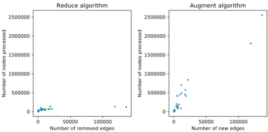
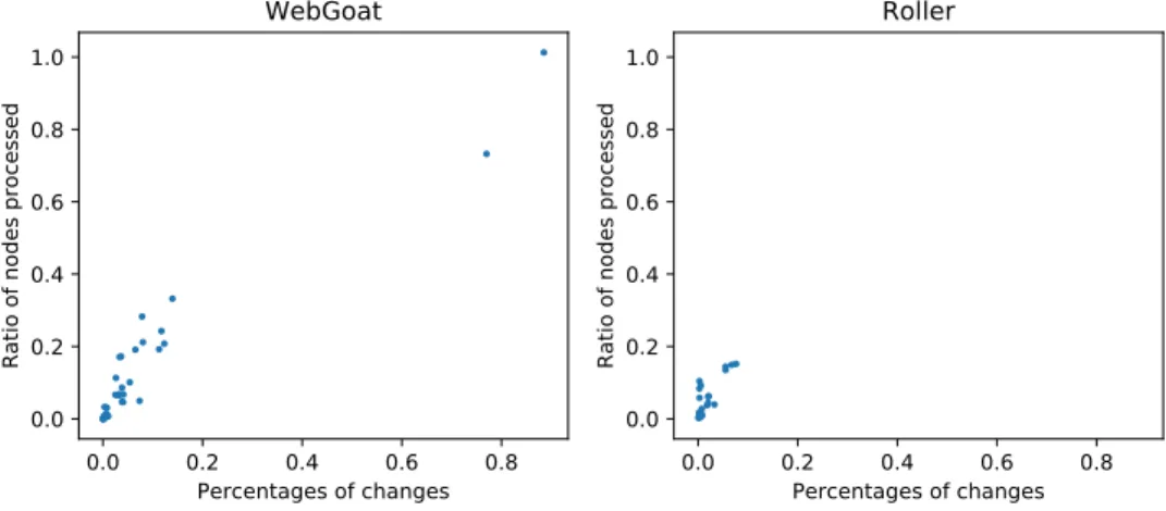
Figure 3.1 Example of SSA instructions forming a control-flow graph . . . 15 Figure 3.2 Example of a data-flow graph . . . 15 Figure 3.3 Example of a converged graph after an execution . . . 23 Figure 3.4 Example of a converged graph after the removal of nodes and edges . 26 Figure 3.5 Example of a converged graph after the addition of a node and an edge 28 Figure 3.6 Impact on incremental analyses in relation to flow changes in WebGoat 35 Figure 3.7 Impact on incremental analyses in relation to flow changes in Roller . 35 Figure 3.8 The ratio of nodes processed in the incremental taint analysis and a
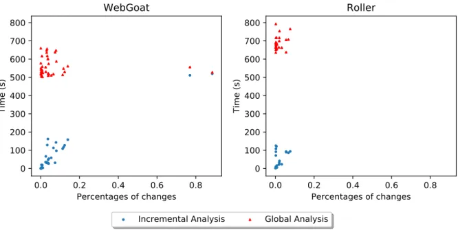
global taint analysis . . . 36 Figure 3.9 The performance of incremental taint analysis and global analysis as
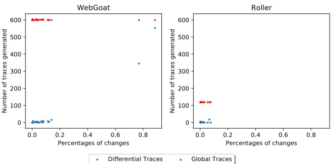
it relates to data-flow changes . . . 37 Figure 3.10 Distribution of traces generated by commit . . . 38 Figure 3.11 Proportion of commits with and without new differential traces . . . 38 Figure 3.12 Performance of differential trace generation as it relates to data-flow
changes . . . 40 Figure 3.13 Comparison of mean time required for a regular analysis compared to
our change-based approaches . . . 42 Figure 4.1 Histogram of nodes traversed for shortest path traces generated with
and without the taint reachability optimization on WebGoat 5.4 . . . 49 Figure 4.2 Histogram of time for shortest-path traces generated with and without
the taint reachability optimization on WebGoat 5.4 . . . 49 Figure 5.1 Example of the integration of the taint analysis tool Cheetah [14] in a
LIST OF SYMBOLS AND ABBREVIATIONS
API Application Programming Interface AST Abstract Syntax Tree
CFG Control Flow Graph DFG Data Flow Graph
FRQNT Fonds de recherche du Québec Nature et technologies IBM International Business Machines Corporation
IDE Inter-procedural Distributive Environment IDFG Inter-procedural Data Flow Graph
IFDS Inter-procedural, Finite, Distributive Subset JDK Java Development Kit
NSERC Natural Sciences and Engineering Research Council OWASP Open Web Application Security Project
RAM Random-Access Memory SCM Source Control Management SQL Structured Query Language SSA Static Single Assignment TAJ Taint Analysis for Java URL Uniform Resource Locator
WALA T.J. Watson Libraries for Analysis XSS Cross-Site Scripting
CHAPTER 1 INTRODUCTION
1.1 Motivation for Change-based Taint Analyses
The work of software developers is frequently at the mercy of ill-intentioned individuals. Hackers try to gain access to systems by all available means because the potential gains are so interesting. A breach in the database of a popular website may easily compromise the private information of millions of users and cause severe damage for both the users and the website. Passwords can be sold to third parties, and stolen credit cards and social security numbers may be used to usurp identities. Web applications, in particular, are sensitive to these attacks and must be designed with care.
Many of these attacks are using injection flaws, which were cited as the most critical secu-rity risk in both the 2013 and 2017 reviews of the Open Web Application Secusecu-rity Project (OWASP) Foundation [5]. This attack consists of injecting untrusted data into a query, like a Structured Query Language (SQL) environment, with the goal of executing an unintended and unauthorized behavior. There are static analyses that exist to try to automatically de-tect these vulnerabilities in the source code. Taint analysis being one of them that simulates how tainted, or distrusted, data is propagated in the software. Developers do not use these analyses as much as they should, since they are framed as slow and imprecise [13]. This is where we want to change things. By reducing the time of a taint analysis, we can remove one of the hindrances of development. A faster taint analyzer could be used in more projects and be performed more frequently by users. We suppose that a more frequent use of such a tool will help detect vulnerabilities sooner and reduce their lifespan, consequently helping to make web applications more secure.
We could play with precision parameters to accelerate an analysis while trying to minimize impacts on the results. However, there is another avenue that could be much more effective: the change-based approach. The evolution of a software project is generally iterative over its course of development. In the lifespan of a project, the source code will evolve in multiple small increments. With each increment, the majority of the codebase remains unchanged. This may not be true for every project and every iteration, but we suspect it is generalized enough to use it to our advantage.
Our proposed solution uses these changes to drive a taint analyzer and update the taint only when needed. It will, as much as possible, utilize the previous results. If the changes in the source code are small, the changes in the results of the analysis should also be small and
reflect changes in the source code.
We will detect the changes concerning security in an application with respect to what can be found with a taint analyzer. This will then be used to report new vulnerabilities to the developers on top of the existing vulnerabilities. A full analysis will report all the vulnerabil-ities detected. However, without an extra step to memorize which of the vulnerabilvulnerabil-ities are new or old, a developer may miss a new vulnerability that has just been added. By using a change-based approach, we can detect very easily which of these are new issues and report them in a way that clearly classifies them as new.
Our motivations for this thesis are: (1) to help developers find the security impacts of changes in source code and (2) to reduce the lifespan of security policy violations in the source code by reducing the computing time of taint analysis.
1.2 Thesis Statement
Prior research [11] has already studied change-based approaches for static analyses, but the taint problem has not been specifically tested; we believe we can provide an alternative that is easier to understand and, possibly, faster.
Our thesis is as follows:
Driven by changes in source code, we can perform more efficient and faster taint analyses by reducing the parts of the graph explored and, subsequently, use it to find impacted vulnerabilities.
1.3 Theoretical Background 1.3.1 Control Flow Graph
Our security analysis, like other data-flow analyses, must follow the flow of the data inside the application. These analyses generally use a Control Flow Graph (CFG) [10]. This graph CF G = hV, Ei has instructions as vertices V , and the edges E consist of all the possible execution paths between the instructions. Such a graph is built from the Abstract Syntax Tree (AST), a data structure representing the overall application and, more importantly, its hierarchical components. It is by exploring the tree and, more precisely, the instructions that we find the control flow edges in the CFG and build it. However, our framework is already giving us the CFG, and we do not have to bother with this part of the analyzer.
1.3.2 Static Single Assignment
In our project, the framework building the control flow graph operates on Java bytecode, and for this reason, instructions use the Static Single Assignment (SSA) form [10]. This alterna-tive format transforms the usual instructions found in the source code into another format to ensure that every variable may not be assigned by more than one instruction. Among other things, this creates a new variable for each assignment, and it adds new instructions to merge the new variables together, when needed, to ensure the same behavior as dictated by the original instructions. Such a form is useful in static analyses because there is only one valid definition for a variable and not multiple ones where we don’t know if they are reachable or not for a given instruction.
1.3.3 Data Flow Graph
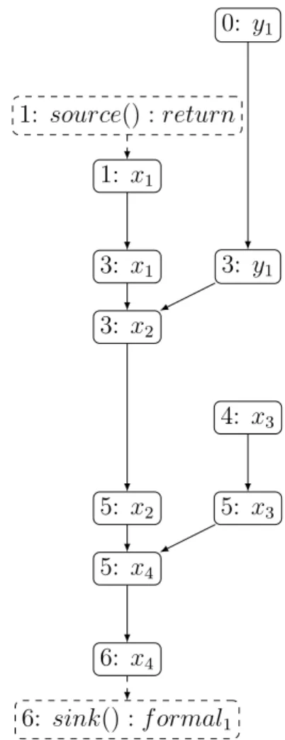
The representation used in our project is different from the CFG. With this last graph, we present another one that specifically represents the data flow. This Data Flow Graph (DFG), DF G = hV, Ei, has, for vertices V , the parameters of every SSA instruction, including the returning value of an instruction. The edges E represent the possible propagations of the data or, in other terms, the links between the definitions and the usages of a variable. For an example, see Figure 3.1 and Figure 3.2 in Section 3.2.1.
1.3.4 Taint
A tainted variable is a variable that may contain unsafe data for an application. In the context of web applications, unsafe data refers to data coming from an external source, like user input or the network, that is not properly sanitized and cannot be trusted.
The goal of our taint analysis is to find such variables in the source code and to detect the vulnerabilities Application Programming Interface (API) with tainted parameters.
1.3.5 Data-Flow Algorithms
Such data-flow algorithms rely on the concept of fixed point. The taint values computed in the graph will grow monotonically until the algorithms converge and reach a fixed point [10]. This occurs by imposing a partial order, or a semi-lattice, to the computed values. In the case of a taint analysis, the variables will generally start untainted, but the algorithm will gradually make them tainted as it explores the graph. For more details about the exact data-flow algorithms and equations, refer to Section 3.2.1.
1.3.6 Trace Generation
We define the term trace as an example of the exploitation of a vulnerability. It is usually represented as an executable path from one instruction to another. In the context of taint, a path would be the ordered set of instructions executed to carry unsafe data from a user input to a vulnerable API. In our experiments, traces are generated for every vulnerability found in the taint analysis.
1.3.7 Source Control Management
Since the algorithms are executed on multiple iterations of the same project, we use a Source Control Management (SCM) tool to fetch these revisions. We chose git [2] since it is a popular tool, and many open-source projects are freely available on this platform. The revisions, or commits, are grouped in pairs to be analyzed in our change-based analysis. The differences between the pairs are generated, and it is these differences that will drive our algorithms.
1.4 Problematic Elements
The main problematic element is the computation time for taint analysis. We analyzed relatively small projects of thousands of lines of code, and our analysis took around 10 minutes for a traditional analysis used as a baseline. This is relatively similar to other research projects [27]. Even if an execution of mere minutes is not bothersome for small projects, industrial projects can have a codebase many times larger than that. For industrial projects, the analysis will not scale well and could take hours to complete, depending on the precision required.
It is important to improve performance, even for small projects. An ideal analyzer should be fast enough to enable interactive feedback inside an integrated development environment. If we succeed at increasing the performance to bring this interactivity, it could help to popularize security tools in the developer workflow. Many developers are not using such tools exactly because of the slow speed of the analyses [13].
Algorithms need to have a sufficient level of precision to bring relevant results. This is crucial in handling the interprocedural propagations since we would miss too many vulnerabilities without it. The strategy chosen to manage this will greatly impact precision and performance [20].
In addition, modern languages have additional mechanisms, which can make our algorithms more complex. The fields of a class need additional logic to precisely propagate the taint. This is similar to precisely propagating a taint over an element of a collection or a pointer modified with pointer arithmetic. The use of statics, exceptions, and many other semantics will all have an effect on the precision of a taint analysis.
In an ideal situation, we want to maintain a somewhat similar level of precision while reducing the time required to compute an analysis. To do such a thing, our solution is to implement a change-based approach. We must use old results as much as possible, find the differences, and limit our computations to the differences and their impacts. The differences must be found in the source code and reflected in the data-flow graphs to compute the taint changes. In a similar fashion, a trace must show an example of every vulnerability found in the taint analysis. The complex elements of taint analysis are also applicable to the generation of traces. It is inefficient to generate the traces of every vulnerability at each analysis and even more so when there is little change in the source code since the last execution. The traces will mainly be the same, and we could simply use the old traces when applicable.
1.5 Research Objectives
Our main research objective is to reduce the computation time of taint analysis. We will implement a change-based strategy to incrementally update the taint values. Our analysis will be driven by the changes in the source code and will limit the scope to only recompute the impacted parts of the DFG.
Our second research objective is to reduce the computation time of the traces. We will implement a change-based strategy to find new traces and limit the generation to only them. Our analysis will be driven by the changes found in the taint analysis.
1.6 Thesis organization
Chapter 2 presents a literature review of various research projects related to taint analysis and incremental strategies used in static analysis. Chapter 3 presents our main article, which describes our innovative, incremental taint analysis algorithms; the experimentations done; and the results obtained. Chapter 4 describes an additional experiment on trace generation that was not included in the article. Chapter 5 is a general discussion of the various subjects of the article. Finally, Chapter 6 is a conclusion summarizing our contributions, our main limitations, and future research.
CHAPTER 2 CRITICAL LITERATURE REVIEW
Multiple projects have worked on improving the speed and reactiveness of static analysis. In this chapter, we present some of these works that are closely related to taint analysis. This chapter focus on the various experimentations that are related to change-based strategies.
2.1 Taint Analysis for Java
The work of Tripp et al. [27] on Taint Analysis for Java (TAJ) was one of the first stepping stones for our current research. They use T.J. Watson Libraries for Analysis (WALA) [9] as a static analysis framework and extended their improvements on top of it. This research has a lot of similarities to the current study because we are both analyzing Java web applications, and we have both collaborated with International Business Machines Corporation (IBM) inside the software IBM AppScan Source [4].
This work is primarily known for the creation of a priority-driven call-graph construction. With this, they can avoid a full computation of their static analyses and give partial results to the user. Their algorithm includes a budget of time and of memory, and under these conditions, the call graph is monotonically generated until the limits are reached. Because of this, the approach under-approximates, which may miss some results. A direct consequence is that their taint analysis is not conservative, but they suggest that the impact on precision is a compromise worth taking.
2.2 Andromeda
The next project, Andromeda [28], is again mainly related to the construction of the call graph. However, Andromeda, which is a direct successor of TAJ [28], is more interesting than TAJ for us. The authors still want to increase the scalability of taint analysis and have improved some of the issues associated with TAJ. Their main contribution is an on-demand approach for their analysis. Important data structures, like the call graph, are no longer eagerly constructed, but a lazier strategy is used instead. Also, the alias analysis is only performed on fields that are tainted. In this new version, their analyses are now sound and conservative.
The next part of their work, which is closely related to ours, is the implementation of incre-mental taint analysis. Their strategy is to recompute all the methods that may have been changed or impacted. One of our main critiques is the lack of detail in which they present
their strategy. It is not clear what they have done, but the granularity of their incremental algorithm seems to be limited to functions. They keep the results of a function when it is not impacted by the changes and recomputes the others. They do not analyze pairs of versions with many changes, only those with small, incremental changes. They add or delete a state-ment or a method and test the response time. Compared to them, we present a replicable approach and measure against code revisions freely available on internet.
2.3 Cheetah
A more recent work is the project Cheetah [14]. While previous projects mainly focused on the scalability of data structures and analyses adjacent to taint analysis, this project is focused on making the computation of the taint itself faster.
They use a priority-driven strategy or, as they call it, Just-In-Time. Usually, data flow analysis starts from the entry points of an application and will compute its flow functions over every statement that is reachable [10]. Cheetah’s approach is somewhat different. Cheetah will also analyze the methods that are unreachable from the entrypoints of the application. This is one of the main points of their strategy, their scanner will starts from the method on which the developer is currently focused and not from an entry point. It is an interactive approach intended to be used while the developer is working on its code.
This is possible because their tool is integrated as an Eclipse plugin. Starting with this method, they can propagate the taint over the statements based on a specific priority. They use a priority queue to order the statements to be processed for computing the taint until a fixed point is reached. Locality is the main factor of importance of a statement for the priority queue. Using this method, a statement of the currently focused function is much more important than a statement accessible over a virtual call. With this, they can find taint on the vulnerable sinks close to the developer’s current point of focus almost instantaneously and report them to the user inside the developer environment.
They have the same goal as us, which is to give to the developer the taint results sooner. Yet, their approach is totally different from our change-based strategy. They have done an integration with Eclipse, and one of their next objectives is to implement an incremental analysis while we have done the opposite.
2.4 Path Verification
On the other hand, Le and Pattison [18] are doing something closer to what we want to accomplish. Their main work is done on the CFG, which is annotated and transformed to contain vertices and edges of multiple versions at the same time. This results in what they call a multiversion interprocedural control flow graph. This is a useful data structure, which they mainly use to verify if a patch has been correctly applied to the version changes. They have developed an incremental analysis for their system, which is able to detect bugs, like buffer overflow and null pointer dereference. For finding the bugs, they use their special CFG, which is incrementally updated from the previous version to a new one corresponding to the changes. They use the cached results of previous analyses, and with them, they query the analyses on the new parts of the graph. However, this procedure is not really developed or explained. They lack algorithms to explain the specific incremental strategy, and they lack performance results to show the improvements over a regular analysis. We present an approach that is more detailed, and we will focus more on the time reduction.
2.5 FlowDroid
One of the most powerful open-source taint analysis engines at the moment is FlowDroid [12]. By integrating some of the previous strategies, like the on-demand approach of Andromeda, they obtained great results and they are scalable for bigger projects. It is a static analysis engine optimized for Android applications and Inter-procedural, Finite, Distributive Subset (IFDS) problems. In fact, multiple recent projects implement IFDS solvers, like WALA [9]. These types of solvers are powerful because they are able to solve classic data flow problems, like reaching definitions, live variables, and other Gen/Kill algorithms, in a polynomial time while being able to handle interprocedural analyses [23].
2.6 Reviser
The authors of FlowDroid tried to improve the performances of the IFDS solver itself. Arzt and Bodden [11] worked on Reviser to make their solver fully incremental for IFDS and Inter-procedural Distributive Environment (IDE) problems. IDE is simply an extension of IFDS that solves more problems and supports more languages [26]. Reviser is an interesting project because it is close to our objective and approach.
They developed an algorithm that uses the changes in the CFG to update the computed values of the data flow analysis impacted by the changes found in the source code [11]. They
have found whether or not the nodes of the CFG are safe, i.e. if it does not have a reachable predecessor that has changed. They will purge the results of the unsafe nodes and repropagate the flow functions on the changed nodes and their impacted neighbors. Finally, they require a second phase where they will again iterate all changed merge points, which are statements with more than one predecessor, to ensure the propagation of unchanged predecessors and ensure valid results.
Reviser is for general IFDS problems and not specialized to taint, so we are different since our experimentations are specific to taint. Also, we differ on the strategy used for the incremental analysis itself. The difference lies in how we update the flow values or, in our case, the taint. They clear the values and compute them again to ensure monotonicity while we replace the clearing by a careful update. This operation will be explained in detail in the following chapters.
CHAPTER 3 ARTICLE 1 : CHANGE-BASED APPROACHES ON TAINT ANALYSES
Nicolas Cloutier, Ettore Merlo and John Peyton Submitted to the Journal of Systems and software Abstract
Modern web applications are sensitive to multiple types of vulnerabilities that put millions of users at risk of having their information compromised. Even if an application’s vulnerabilities were all eliminated at some point, there would still be a risk of introducing new vulnerabilities when it is updated. Code review and other manual techniques, as well as automated methods, such as static analysis, can be used to find new defects. However, since performance is an issue, they are usually not performed on every commit but executed daily by an integration server or manually by a security expert.
This is why we propose novel change-based approaches to perform faster inter-procedural taint analyses in the context of software development. An evaluation of timings on the open-source projects WebGoat and Roller shows performance gains of 90 to 95% on our analyzed projects compared to the analysis without the incremental improvements. This dramatic reduction in the required computation time would enable developers to quickly analyze code changes and detect potentially threatening vulnerabilities.
Keywords
inter-procedural static analysis, taint analysis, incremental analysis
3.1 Introduction
Web applications are similar to other software programs, such as mobile applications, video games, and embedded systems, and may be the target of multiple attacks since they contain sensitive data desired by hackers. They are at risk due to their exposure to public networks and need security policies to ensure the confidentiality, integrity, and availability of data [22]. A policy is a formal or informal description of the processes and mechanisms used to partition and secure a system. Vulnerabilities are violations of these policies, which can be dangerous, especially when they are exploited, and lead to unexpected behaviors. Briefly, vulnerabilities can be classified into two categories: application vulnerabilities and environmental
vulner-abilities [6]. Application vulnervulner-abilities arise from the program itself, while environmental vulnerabilities are violations caused by something external to the application, for example, the absence of segregation on an internal network for critical systems.
Application vulnerabilities are generally caused by either faulty code or design flaws [6]. SQL injection, Cross-Site Scripting (XSS), and unintended authentication are known examples [5] of this type of violation. We are specifically interested in data-driven vulnerabilities where external data, which may be malicious, is propagated to critical parts of the system.
Data-driven vulnerabilities are interesting since static analysis techniques like taint analysis can preemptively detect some of these [28]. Taint analysis is used to detect violations of policies by finding paths between external sources and vulnerable calls to API. To find these paths, we generate a justification in the form of a trace, presented to the developer. These traces have the goal of explaining how the vulnerability can be exploited by showing an example of how it is propagated in the application. We focus our research on improving the taint analyses and the traces generation.
Performing taint analyses may require a significant amount of time on large systems due to the volume of code to analyse and traditionally do not scale well [27]. It is possible to perform the analyses more quickly by trading precision for better performance [27], but it could deter developers from using these tools [13].
Another way to make them faster while avoiding a trade-off is using change-based approaches [11, 19, 24]. Change-based approaches are strategies that detect changes between pairs of versions and reflect changes in the analyses to avoid computation of unchanged results. It is a more generic term and includes, for example, incremental and differential analyses.
A differential analysis will detect changes, discards the analysis results affected by the changes, and then repeats the analysis to re-computes the missing analysis results. An in-cremental analysis, however, does not discard the results; it updates them. The first method is limited to finding differences, while the latter goes one step further and uses the differ-ences to incrementally perform a computation. Other approaches, such as on-demand and partial analysis [28], control and limit when and where a computation occurs. They are not necessarily change-based, but it is possible to combine them [14].
As already reported by multiple researchers [11, 19, 24], one of the main opportunities to improve data-flow analyses is considering the incremental nature of software development. Programs evolve with multiple small iterations, and we expect them to remain the same with some small modifications after each new revision, but exceptions may exist for major revisions or major refactoring. Therefore, we should expect the results of a program’s static
analyses to be quite similar and the differences to reflect changes made in the code. We will account for the evolutionary nature of software development and present new and original change-based approaches to improve inter-procedural data-flow approaches for taint analysis. By reducing the amount of time required to perform computations that analyse the impact of code changes, we hope to be more time efficient and improve the algorithms’ scalability for industrial software.
Our incremental and differential algorithms perform comparisons of pairs of software versions. Commonly, a pair of versions includes two commits coming from source control where one version is the oldest and the other is the newest. Our analyses store the static analysis results of versions and use it as a starting point for the next analysis. When a change-based analysis is triggered, changes in the flow graph are computed from differences in the source code, and their impact on taint and other analyses results are conservatively computed.
To present our change-based approaches, the paper is structured as follows. Section 3.2 in-troduces and provides a detailed description of our novel strategy to incrementally update a taint analysis. Section 3.3 explains how we can directly use the results of an incremental taint analysis to accelerate trace generation. Section 3.4 explains the experiment’s methodology, while Section 3.5 presents and discusses the results. Threats to validity are discussed inSec-tion 3.6, and related works are discussed in SecinSec-tion 3.7. Finally, conclusions are presented in Section 3.8.
3.2 Incremental Taint Analysis
3.2.1 Main concepts of taint analysis
In this subsection, we define the main concepts related to taint analysis. A reader may skip these concepts and go directly to the next subsection if desired.
Our system builds a control-flow graph CF G = hVCF G, ECF Gi where the vertexes VCF G are static single assignment (SSA) instructions, and the edges ECF G represents how flow control can be transferred between SSA nodes. Figure 3.1 is an example of possible SSA instructions. We also create another representation as a data-flow graph DF G = hVDF G, EDF Gi of the SSA arguments. In this graph, the vertexes VDF G represent each parameter of an SSA instruction. The directional edges EDF G represent how data flow from one parameter to another. For every use of a defined node, an edge is created. When we use the terms successor and predecessor, we usually refer to the vertexes connected by an edge to a vertex of the DF G. A predecessor of a node is another node in the DF G which can be the origin of the data. A successor of a node is another node in the DF G where the data can be propagated into. The dashed lines
and nodes handle the inter-procedural aspects, which are detailed in Section 3.2.3. For the CFG in Figure 3.1, the corresponding DFG is Figure 3.2.
In the context of this research, the meaning of ’taint’ is close to the concept of contamination. We define a tainted variable as a variable that can contain external and untrusted data that has not been properly sanitized. Such a variable could be corrupted by a malicious user to ultimately violate established security policies. Our analyses operate on DF G, and the taint will be computed for every node in VDF G.
A taint source defines a function, or an API, which returns untrusted data. Usually, it is any function that returns values coming from a user or the network. We mark the return value from a source as tainted. Subsequently, the variables that the return value can flow into will also be tainted. Validators (or downgraders [25]) enforce security policies. They are special functions that “downgrade” the level of taint. In the case of SQL injection, they will sanitize the input by, for example, escaping specific characters, such as apostrophes, and make it safe to use for SQL queries. We represent the taint in function of sources and validators formally in Equation 3.1.
For any node n in VDF G, it is tainted if a path p exists in the DF G from a source n0 and this
node n. n0 is another node of the DF G, which is also in the set of sources. To be tainted,
there should not be any node in the path nx, which is in the sets of validators. Such a path bringing taint from a source to a node may also be called an unprotected path. A protected path means that the taint from the source is blocked by a validator. If all the paths from the sources to a node are protected by validators, we cannot mark the node as tainted.
T aint(n) =
T rue ∃phn0,...,ni ∈ DF G such that
n0 ∈ sources ∧ 6 ∃nx ∈ p | nx ∈ validators F alse otherwise
(3.1)
However, if a node executing a SQL query is tainted, it has a possible vulnerability. We call such vulnerable APIs a security sink. As indicated in Eq. 3.2, a vulnerability exists only if a node n of the DFG is tainted and is a sink or in a set of sinks.
V ulnerable(n) =
T rue T aint(n) ∧ n ∈ sinks F alse otherwise
(3.2)
Our goal is to compute the taint in all nodes of the data-flow graph, and to detect tainted sinks, we need data-flow analyses. In the literature [10], a standard data-flow analysis
frame-EN T RY 0: y1 = ”f oo” 1: x1 = source() 2: if cond() 3: x2 = x1+ y1 4: x3 = ”bar” 5: x4 = phi(x2, x3) 6: sink(x4) EXIT
Figure 3.1 Example of SSA instructions form-ing a control-flow graph
0: y1 1: source() : return 1: x1 3: x2 3: x1 3: y1 4: x3 5: x4 5: x2 5: x3 6: x4 6: sink() : f ormal1
work has been defined to work on flow graphs of basic blocks, and derived from this format, we can define an iterative algorithm to compute the taint over the SSA instructions with Al-gorithm 1. The main parameters for this forward alAl-gorithm are the domain of values VDF G, flow equations fD, and meet operator ∨.
Algorithm 1 Iterative algorithm for a forward data-flow taint problem 1: for each vertex D from the DFG VDF G do
2: OU T [D] = ⊥
3: while changes to any OU T occur do
4: for each vertex D from from the DFG VDF G do
5: IN [D] =W
P a predecessor of DOU T [P ]
6: OU T [D] = fD(IN [D])
The dictionary OU T contains the taint processed for every vertex of VDF G, and IN is some-what similar. It corresponds to the inputted taint coming from the predecessors of a vertex. The values computed over the domain VDF G are represented by a simple boolean lattice. It does denote whether the variable related to a vertex is tainted [15, 27]. The Boolean value F alse means untainted, and T rue means tainted.
In the algorithm, we chose to iteratively propagate the taint from the sources to the sinks. It is a forward approach. As previously defined in Equation 3.1, a node is tainted if a path exists between a source and node without a validator on the path. For our algorithm, this means that the meet operator ∨ must be a logical disjunction ∨. If a predecessor of a node is tainted, the value contained in IN for this node must also be tainted, as represented in Equation 3.3. In(D) =
T rue if ∨p∈predecessors(D)Out(p) is true F alse otherwise
(3.3)
We will define the flow equations fD as follows in Equation 3.4. It is a modified version of GEN & KILL functions as seen in the literature [10], but it is adapted to Boolean logic. It does receive the Boolean taint value x for a node D as an input and computes the taint. It does use two functions, Gen(D) and Kill(D), which are defined in the following equations.
fD(x) = Gen(D) ∨ (x ∧ ¬Kill(D)) (3.4)
To do so, it needs a set sources of the existing sources. The kill function (Equation 3.6) will stop the propagation of taint if the current node is a validator. If a node is in the set of validators validators, the returned value for the KILL function is true so that the flow equation outputs a taint value equal to false. Subsequently, the function fD(x) will return the taint for a node as true if either the node is a source or the inputted value is tainted and not killed by a validator.
Gen(D) = F alse if D 6∈ sources T rue if D ∈ sources (3.5) Kill(D) = F alse if D 6∈ validators T rue if D ∈ validators (3.6)
Since we are generating new taint and propagating it over the graph, the starting values must be equal to ⊥ or not-tainted. By iteratively marking nodes as tainted and never unmarking a node, we ensure a monotonic algorithm and eventually converge to a fixed point.
3.2.2 Equivalent classes of sinks
Since validators are used to enforce only a subset of security policies, they will only protect a subset of the sinks. A validator for SQL injections will transform strings to make them harmless for an SQL query function, a sink. However, for another sink, it may not perform a sufficient protection. Consequently, the taint is different depending on the sink analyzed. The previous equation 3.1 of taint should be modified to include this detail in Equation 3.7. It is modified to associate the taint with sinks and only downgrades when a validator related to the sinks exists in the path. It is done by having validators(s), which return the set of validators that can protect a sink s. The other variables are identical to those defined in Equation 3.1. SinkSensitiveT aint(n, s) =
T rue ∃phn0,...,ni ∈ DF G such that
n0 ∈ sources ∧ 6 ∃nx ∈ p | nx ∈ validators(s) F alse otherwise
(3.7) As taint must be considered differently for every sink (i.e., API) analyzed, Eq. 3.7 should be computed for every distinct type of API.
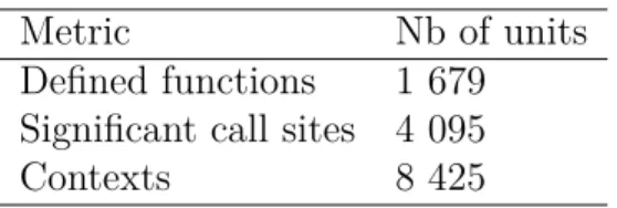
Repeating the computation of taint can become time-consuming. To give an idea of the number of analyses required, on the version 5.4 of WebGoat, an open-source project which we will talk more about in Section 3.4, there are 42 different API sinks and 37 validators. So taint analysis should be repeated 42 times for the whole application.
By investigating different APIs, we found that most of them seem to behave in a similar manner in terms of taint. For example, there are multiple sinks related to SQL, and they interact identically with all the validators. For these sinks, the set of validators that down-grade the taint is equal. In this case, it is possible to construct equivalent classes and group them together to reduce taint analysis computation effort. If the number of equivalent classes is low, it will drastically reduce the computations since a taint analysis is required for every class.
As presented in the equations (3.8), we provide the following definitions. A validator v is in the validators V alss of a sink s only if this API validator blocks the taint for this API sink. Similarly, a sink s is also in the set of sinks Sinksv of a validator v when the taint is blocked for this sink and validator combination.
A sink s is in an equivalent class of sinks Se if and only if they are protected by exactly the same set of API validators.
A validator v is in an equivalent class of validators Ve if and only if they protect exactly the same set of API sinks.
v ∈ V alidatorss ⇐⇒ doesV alidate(v, s) = T rue s ∈ Sinksv ⇐⇒ doesV alidate(v, s) = T rue
s ∈ Se ⇐⇒ ∀s0 ∈ Se(V alidatorss0 = V alidatorss) v ∈ Ve ⇐⇒ ∀v0 ∈ Ve(Sinksv0 = Sinksv)
(3.8)
For the projects analyzed in this paper, we computed that the number of equivalent sinks and validators was much smaller than the number of APIs. By performing a brute-force comparison of every sink and validator, we obtained a maximum of five distinct groups of equivalent sinks and three groups of equivalent validators. For example all the sinks and validators for SQL injections are now grouped toghether.
These groups are used in our algorithm by simply replacing the sink for Equation 3.7 with the corresponding class of equivalence. Consequently, the kill equation (3.6) is modified to use validators corresponding to the current equivalency class of sinks.
analyses without these classes. On this reduced computation analysis, we observed the same tainted sinks at a fraction of the computation time normally required. We passed from 72 minutes to 9 minutes for our analysis.
3.2.3 Implementation of standard taint analysis
Based on the previously defined equations for taint, we designed the Algorithm 2 and im-plemented it using the application IBM Security AppScan Source [4]. In this algorithm, the successors function takes as a parameter an element of VDF G and returns a subset of the VDF G where successors(n) = {s|(n, s) ∈ EDF G}. Similarly, the predecessors function has the same domain and image, but the subset returned corresponds to predecessors(n) = {p|(p, n) ∈ EDF G}. EDF G is given by our framework and enables us to avoid the management of complex mechanisms, such as fields.
An Inter-procedural Data Flow Graph (IDFG) is an alternative version of the data-flow graph used for our inter-procedural analyses and is discussed below in Section 3.2.4.
According to Algorithm 1 defined in Section 3.2.1, we iterate every vertex from the DFG repeatedly until a fixed point is reached. This approach is inefficient and can be improved. A better strategy would be to find the analyzed sources in the project and begin our com-putation from this set. To detect the sources, we must start from the entry points in the application, typically the main function, and recursively search in the code for the source API. This improvement is reflected in lines 5-7 and the Algorithm 3. The function F etchAllInterprocContexts(source) used take a source and retrieve all the corresponding nodes in the inter-procedural data-flow graph (IDFG).
In Algorithm 1, we iterate VDF G repeatedly until a fixed point is reached. It is possible for our problem to compute the same results with a work list. It is valid since the only nodes impacted by a change of taint are the transitive successors of the node impacted. By queuing all the successors when a change occurs, we ensure the correct result is eventually achieved. We expect such a modification to accelerate our computation.
3.2.4 Inter-procedural strategy
Obviously, this new algorithm needs to be inter-procedural, since programming languages have procedures that determine how data can be propagated.
One approach for a fully precise analysis would clone, or inline, the graph of each function for every possible call stack [10]. In practice, this approach is not feasible in a reasonable amount of time for programs with a relevant size [20]. However, an insensitive strategy would not
Algorithm 2 Global fixed-point taint analysis 1: procedure GlobalAnalysis(idf g, entrypoints)
2: for all n ∈ idf g do . Initialization of taint for every node 3: taint[n] ← F alse
4: worklist ← List() . Push the sources to launch the analysis 5: for all source ∈ ReachableSources(entrypoints) do
6: for all node ∈ F etchAllInterprocContexts(source) do 7: worklist.push(node)
8: while ¬worklist.empty() do 9: c ← worklist.pop() 10: if c ∈ sources then 11: inT aint ← T rue
12: else if c ∈ validators then 13: inT aint ← F alse
14: else
15: inT aint ← F alse
16: for all p ∈ predecessors(c) do 17: inT aint ← inT aint ∨ taint[p]
18: if inT aint ∧ ¬taint[c] then . Inside the if the node is tainted 19: taint[c] ← inT aint
20: if c ∈ sinks then
21: Report tainted sink 22: for all s ∈ successors(c) do
Algorithm 3 Search of reachable sources 1: function ReachableSources(entrypoints)
2: reachableSources ← Set() 3: visited ← Set()
4: q ← Queue()
5: for all entrypoint ∈ entrypoints do 6: q.enqueue(entrypoint)
7: while ¬q.empty() do 8: f unction ← q.dequeue()
9: for all node ∈ df g(f unction) do 10: if node ∈ sources then
11: reachableSources ← reachableSources ∪ node 12: if isCallSite(node) then
13: for all calledF unction ∈ called(node) do 14: if calledF unction 6∈ visited then
15: visited.insert(f unction)
16: q.enqueue(calledF unction)
return reachableSources
propagate values over the inter-procedural edges and only resolve what is inside a procedure. We have chosen to compute the taint of a function and the related inter-procedural edges separately for every existing call site. This strategy offers a balance between speed and the precision of results for our analysis.
Let the inter-procedural data-flow graph IDF G = (V, E) be an exploded version of the data-flow graphs (DFG). The IDFG is a graph containing every clone created for inter-procedurality. A clone will be created for a function for every existing context, which is the call-site of the caller. For every context, an inter-procedural edge is created from the parameter node of the calling function to the formal parameters of the called functions. An edge will also be created from the return value of the called function to the actual return value at the call-site.
One important aspect of modern languages affecting our algorithms is the use of polymor-phisms. Virtual calls can be analyzed to narrow the set of possible called functions. Our work environment is already providing us with a virtual call resolution, and the results are used directly by our analyses.
By using the context-sensitive strategy of creating a clone for every caller-callee pair possible, the size of the IDFG should be multiple times larger. Furthermore, the time required to compute the taint should also be considerably longer. We must also remember that a separate
analysis must be performed for each equivalent class of sinks present in an analyzed project. However, we have an algorithm that can be used as a baseline in our experiments against our incremental algorithms.
For a single run of our analysis, a node can be processed multiple times by the main while loop (Line 8) of Algorithm 2. First, source nodes will be added to the work list to begin the computation. Second, a node computed in the work list can push its successors in the work list only when the taint increases, which can only happen once and is enforced by the condition at line 18 of the algorithm. In the worst case, all of the nodes in the IDFG will be reachable from the sources and will be treated by the algorithm.
3.2.5 Road to an incremental approach
An incremental taint analysis takes the flow values from previous analyses and uses them as a starting point. In this section, we will describe how our algorithms implement this idea. Incrementally updating a taint analysis will bring new complexities, such as handling multiple versions of source code and the need for new algorithms capable of handling the differences. We want to reduce the number of nodes processed to only the nodes impacted by changes, but we must ensure our new algorithms will find the same set of tainted sinks compared to our baseline analysis. Even with these constraints, we want to investigate whether, like similar projects that had good results [11], an incremental analysis can be faster than our baseline analysis on an average pair of versions.
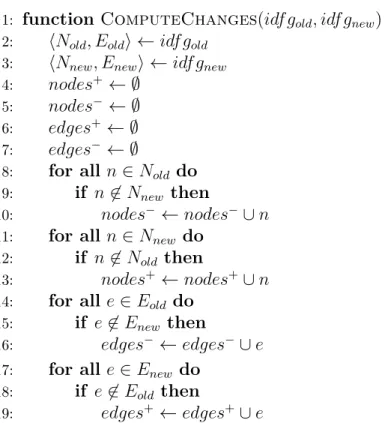
Furthermore, we have a differential tool that works on a pair of versions and computes the changes in the IDFG between the pair. Algorithm 4 is a generic approach used to compute various sets between the pair. This generic approach is expensive but can be improved, for example, if the developer environment is keeping track of the changes as they occur.
Our incremental algorithm is based on the strategy of juxtaposing the impacts of every change. In this section, we explain how we juxtapose the effects of removals and additions in the graphs to update the taint.
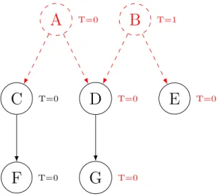
Consider an example on Figure 3.3 with a taint already computed on it. In this graph, the node B is tainted, thus its reachable successors, D, E, and F, are all tainted as well since there are no validators to block the propagation. It will be used later as a small example of incremental analysis.
Considering the equation of taint presented in Equation 3.1, the taint is the existence of an unprotected path from a source to a node. For any node in the graph, the removal of another node or an edge will only affect the taint value if it is in a tainted path between
Algorithm 4 Diff algorithm 1: function ComputeChanges(idf gold, idf gnew)
2: hNold, Eoldi ← idf gold
3: hNnew, Enewi ← idf gnew
4: nodes+ ← ∅ 5: nodes− ← ∅ 6: edges+ ← ∅ 7: edges− ← ∅
8: for all n ∈ Nold do
9: if n 6∈ Nnew then
10: nodes−← nodes−∪ n 11: for all n ∈ Nnew do
12: if n 6∈ Nold then
13: nodes+← nodes+∪ n 14: for all e ∈ Eold do
15: if e 6∈ Enew then
16: edges−← edges−∪ e 17: for all e ∈ Enew do
18: if e 6∈ Eold then
19: edges+← edges+∪ e
return hnodes+, nodes−, edges+, edges−i
A
T=0B
T=1C
T=0D
T=1E
T=1F
T=0G
T=1the source and the node in question. If the removal is not in the transitive predecessors, it cannot impact the taint. Subsequently, if a part of the graph is removed, the impact on the taint will be limited to the successors of the removed part.
Another characteristic of a removal is that it can only reduce the value of the taint. Reducing is the action of changing the taint value from true to false. Considering the implication in Equation 3.9, an untainted node n implies that the node is a validator or that no predecessor p is tainted.
T aint(n) = F alse =⇒ n ∈ validators∨ 6 ∃p ∈ predecessors(n)(T aint(n) = T rue) (3.9)
If the node is a validator, the taint will never be true regardless of how much the predecessors change. If no predecessors are tainted, the removal of one of them cannot taint their successor. Furthermore, the removal of any of these predecessors will always result in an untainted successor.
If the successor n of a removed edge is tainted, it is because at least one predecessor p was tainted or that n was a source (Equation 3.10).
T aint(n) = T rue =⇒ n ∈ sources ∨ ∃p ∈ predecessors(n)(T aint(n) = T rue) (3.10)
The removal of a predecessor will reduce the taint if it was the only tainted predecessor; otherwise, it will stay the same since a tainted predecessor still exists. Also if it was a source, the removal of a predecessor will not remove the taint, and it will remain. Hence, the removal of an edge can only retain or reduce the taint in a graph. If we remove all the edges and nodes that are to be removed because of an incremental update, the overall computation will be monotone.
The update of the taint caused by removals is implemented in Algorithm 5, which also uses this strategy. It is nearly identical to the regular algorithm. This algorithm is designed to operate on the new iteration of the program and the parameter IDF G corresponds to this new iteration. It no longer has the removed nodes and the removed edges in the graph itself, but with the help of the stored results and Git, we can still retrieve them to operate our algorithms. This is important for the initialization of the work list. We only push the nodes when their taint could possibly be reduced (i.e., the successors of removed edges that still exist in the new version).
The line 3 iterates the removed edges and 4 ensures we do not push a node that no longer exist in the current version. As previously mentioned, we want to only handle the removal of parts of the graph; it is important to momentarily ignore the new edges in the graph. If we did not ignore the new edges, we could no longer guarantee that the taint can only be unchanged or reduced. If the algorithm could also increase the value of the taint, it would no longer ensure the monotonicity of our algorithm, and it may never reach a fixed point. The conditions at line 15 and 21 ensure that we ignore them. Finally, we do not have to report newly tainted sinks since it is impossible when only reducing taint.
Algorithm 5 Incremental reduce fixed-point taint analysis 1: procedure ReduceAnalysis(idf g, nodes−, nodes+, edges−, edges+) 2: worklist ← List()
3: for all hp, si ∈ edges− do 4: if s ∈ idf g then 5: worklist.insert(s) 6: while ¬worklist.empty() do 7: c ← worklist.pop() 8: if c ∈ sources then 9: inT aint ← T rue
10: else if c ∈ validators then 11: inT aint ← F alse
12: else
13: inT aint ← F alse
14: for all p ∈ predecessors(c) do 15: if hp, ci 6∈ edges+ then
16: inT aint ← inT aint ∨ taint[p] 17: if inT aint ∧ ¬taint[c] then
18: taint[c] ← inT aint 19: if c ∈ sinks then
20: Report tainted sink 21: if hc, si 6∈ edges+ then
22: worklist.insert(s)
If we apply this algorithm to Figure 3.3 with the removal of nodes A and B and their respective edges, we will obtain a graph like the one in Figure 3.4. This will simply result in a graph where all the taint values have been reduced to untainted since B was the only source of taint. The only nodes unchanged would be C and F because they are not reachable successors of B. C will be processed because of the removal of A but not its successor F since C did not update its taint. In this scenario, F would be the only node excluded by our algorithm.
A
T=0B
T=1C
T=0D
T=0E
T=0F
T=0G
T=0Figure 3.4 Example of a converged graph after the removal of nodes and edges
Like the removal of an edge, the addition of a new edge or a new node may only impact the nodes that are reachable by using the successor’s edges transitively. Again, considering the equation of taint (3.1) on any node, the addition may only have an impact if it creates an unprotected path.
Similar to the removal of an edge or a node, the addition of a new element to the graph can only augment the taint values in the graph. It can only augment the taint from false to true. As described previously in Equation 3.10, a node is tainted only if it is a source or it has a tainted predecessor. The addition of a new predecessor cannot change the fact that a tainted predecessor exists.
Finally, if a node is not tainted, the addition of a node or an edge cannot further reduce the taint value. As said in Equation 3.9, an untainted node is either a validator or did not have any tainted predecessor. If the node is a validator, the addition of a predecessor changes nothing, regardless of whether it is tainted. If there was no unprotected path previously, the taint will be equal to the taint of the new predecessor. If the new predecessor is untainted, it means there is still no unprotected path that can reach this node. If the predecessor is tainted, it means that an unprotected path now exists.
By using these together, if we only compute the new edges and new nodes that will be created because of an incremental update, the overall computation will be monotonous and only increase the taint in the graph. The update of the taint for the addition of new edges and new nodes is implemented in Algorithm 6. Compared to the baseline algorithm, we only have to initialize the taint value of the new nodes and push the nodes possibly impacted by the addition of edges. These nodes are the successors of new edges and the new nodes
themselves. This ensures that a new source without predecessors will be computed and correctly propagated. The default taint of the new nodes is set to untainted since the other choice would break the monotonicity.
Algorithm 6 Incremental augment fixed-point taint analysis 1: procedure AugmentAnalysis(idf g, nodes−, nodes+, edges−, edges+) 2: for all n ∈ nodes+ do
3: taint[c] ← F alse 4: worklist ← List() 5: for all n ∈ nodes+ do 6: worklist.insert(n) 7: for all hp, si ∈ edges+ do 8: worklist.insert(s)
9: while ¬worklist.empty() do 10: c ← worklist.pop() 11: if c ∈ sources then 12: inT aint ← T rue
13: else if c ∈ validators then 14: inT aint ← F alse
15: else
16: inT aint ← F alse
17: for all p ∈ predecessors(c) do 18: inT aint ← inT aint ∨ taint[p] 19: if inT aint ∧ ¬taint[c] then
20: taint[c] ← inT aint 21: if c ∈ sinks then
22: Report tainted sink 23: for all s ∈ successors(c) do
24: worklist.push(s)
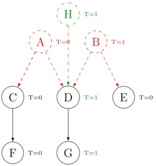
Starting from the results of Figure 3.4, we add a new tainted node H and link it to the existing node D. We obtain the final computation as given in Figure 3.5. In this example, only the nodes H, D, and G will be processed and updated. The other nodes are not reachable from H and do not require validation. Using this brief example, a complete full analysis would have given the same results. C, E, and F would have been set to untainted, while D, G, and H would have been set to tainted.
By successively using Algorithm 5 and Algorithm 6, we iteratively compute the taint of every change until we reach a fixed point to obtain the updated taint of our analyzed application.
A
T=0B
T=1C
T=0D
T=1E
T=0F
T=0G
T=1H
T=1Figure 3.5 Example of a converged graph after the addition of a node and an edge
3.2.6 Research Questions:
RQ1: Given a set of version pairs found in existing projects, what is the ratio of nodes processed between an incremental analysis and a baseline analysis to compute the newest version? Additionally, with respect to the amount of source code changes and the taint impact of changes.
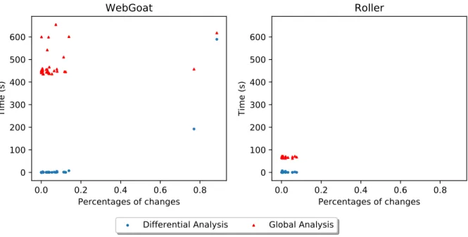
We assume a commit is generally a small increment from the last version. In most cases, modifications made by a developer should be small compared to the total size of the system. Our strategy would become advantageous when we only process nodes impacted by the changes in the flow graph, but how does this impact compare to our baseline analysis? RQ2: How is incremental analysis faster in practice than a global analysis? Even if the impact in terms of the number of nodes processed is low, the speed of our incremental analysis may be slower than a global analysis. The algorithms have additional instructions that may negatively impact the speed of the analysis. In practice, how does the computation time compare for the two approaches?
3.3 Differential Trace Generation 3.3.1 Trace Generation
With our taint analysis approach, developers will know which functions are currently vul-nerable, but they may have difficulty finding the root cause of why a function in the code is vulnerable. A root cause is flawed code that must be fixed to protect a vulnerable sink. We generate examples of unprotected paths to help developers identify this type of code. Traces are examples generated by our algorithms. In this section, we discuss trace generation and how change-based techniques can be used to our advantage to improve the process.
For a given sink, we could try to generate an example for all the unprotected paths. However, it would be impossible to compute without approximations due to the presence of cycles in the DF G. Even with approximations, developers will probably be overwhelmed by all the information [21]. If only one path is displayed, other unprotected paths may not be fixed immediately, and the developer will only find out in the next analysis, which might be annoying if the amount of time required to complete the analysis is lengthy. Another parameter to consider is the amount of time required to generate individualized traces based on the chosen trace generation strategy.
When displaying traces to the user, we must choose the most relevant ones to help the developer identify the root cause. Researchers have identified some practices that can help make a trace more meaningful for the user: (1) Shorter traces are more efficient than longer ones [17]; (2) The traversal of a call site for a polymorphic function should be avoided since it has a higher chance of creating false positives [20]; and (3) The overall number of functions traversed should be minimized to increase the locality of the trace [16].
All paths
To pseudo-generate all the unprotected paths in Equation 3.11, we must search for all the paths p from any source no to the sink ni that does not contain a validator. This approach can generate an enormous number of paths and can be infeasible if we do not ignore some traces. In the generation process, we need to ensure that a node can only be present once in the path. Otherwise, the number of paths for any looping graph will be infinite. If the path A-B-C-B-D exists, and non-unique nodes are not imposed, the path A-B-C-B-C-B-D should also exist. In consequence, we could find an infinite number of paths for this brief example by adding the edges B-C-B repeatedly. To avoid this problem, we use the algorithm designed by Princeton for a simple generation of all the unprotected paths without cycles [8].
∀p(no,...,ni)∈ IDF G{no∈ sources ∧ ni ∈ sinks∧ 6 ∃nx ∈ p(nx ∈ validators) =⇒ p ∈ AllT races(ni)}
(3.11)
Shortest path
An easier approach than searching all paths would be to find the shortest unprotected path for each sink. The shortest path fits the predicate in the Equation 3.12. It is implemented as a form of breadth-first traversal but could be done differently [29]. The algorithm will start from the tainted sink and iterate over the predecessors to find the source. It will also remember the nodes traversed to reduce the number of nodes traversed. It will permit backtracking to the sink at the end and generate the shortest path. The algorithm 7 is used over the IDFG.
∀p ∈ AllT races(ni){6 ∃px ∈ AllT races(ni)(|px| < |p| ∧ px 6= p)
=⇒ p = ShortestT race(ni)}
(3.12)
Spanning tree
An alternative to the generation of unprotected paths is spanning trees. This approach can find multiple paths rather than just the shortest path and does not take as much time as an excessive all-paths generation. We define our spanning tree as a tree covering all the tainted nodes in the IDFG reaching a given sink. Additionally, there is no notion of weight in our graph. The spanning trees can be computed with Algorithm 8.
3.3.2 Differential Strategy
Like taint analysis, the exhaustive generation of traces can be improved with change-based approaches.
For the traces, we will use a differential analysis to ignore previously tainted sinks and only generate traces for newly tainted sinks. We give the developer only the new traces that are created by his recent changes. Although the details are not included here, it is possible to report the sinks that have been protected.
Due to time limitations, only the approach for shortest path generation has been tested, and future research is needed to investigate the other strategies.