Post-Surge Flow Prediction in Multi-Stage Compressors

(1)

UNIVERSITÉ DE MONTRÉAL

POST-SURGE FLOW PREDICTION IN MULTI-STAGE COMPRESSORS

JAVAD HOSSEINI

DÉPARTEMENT DE GÉNIE MÉCANIQUE ÉCOLE POLYTECHNIQUE DE MONTRÉAL

MÉMOIRE PRÉSENTÉ EN VUE DE L’OBTENTION DU DIPLÔME DE MAÎTRISE ÈS SCIENCES APPLIQUÉES

(GÉNIE MÉCANIQUE) AVRIL 2015

(2)

UNIVERSITÉ DE MONTRÉAL

ÉCOLE POLYTECHNIQUE DE MONTRÉAL

Ce mémoire intitulé :

PRÉDICTION D’ÉCOULEMENT DANS DES COMPRESSEURS MULTI-ÉTAGÉS DURANT LE POMPAGE

présenté par : JAVAD HOSSEINI

en vue de l’obtention du diplôme de : Maîtrise ès sciences appliquées a été dûment accepté par le jury d’examen constitué de :

M. MUREITHI Njuki, Ph. D., président

M. VO Huu Duc, Ph. D., membre et directeur de recherche M. REGGIO Marcelo, Ph. D., membre

(3)

DEDICATION

(4)

ACKNOWLEDGEMENTS

I would like to express my deepest appreciation to Prof. Huu Duc Vo for his guidance and support for me and my research.

I am grateful to my parents, my brother and my wife, who have continuously encouraged me in my study and in my life.

I worship my small children, their hands waiting to touch their daddy’s hands who in return kisses their small hands when they sleep.

I would like to show my appreciation to the people who though their positive wishes always encouraged me.

I would like to express my gratitude to Prof. S. Rasouli who was my former advisor in undergraduate study.

I am thankful to my brilliant colleagues, Noureddine Djeghri, Farzad Ashrafi and Martial Dumas. Last but not least, I would like to thank to all people who contribute their life to technological progress. The life we have today is the result of their endless effort.

(5)

RÉSUMÉ

Le pompage est une instabilité aérodynamique uni-dimensionnelle dans une turbine à gaz caractérisée par l’apparition de pulsations axiales allant jusqu’à une inversion globale du sens de l’écoulement et qui est très dommageable pour la performance de l’intégrité physique du moteur d’avion. La capacité de prédire les propriétés de l’écoulement pendant le pompage à différents endroits dans le compresseur aiderait les concepteurs à optimiser le design de plusieurs composantes du moteur pour mieux résister aux forces aérodynamiques impliquées.

L’objectif de cette recherche est de développer une méthode rapide et efficace pour prédire la fluctuation des propriétés de l’écoulement à n’importe quelle section dans un compresseur multi-étagés et qui serait utilisable au stage préliminaire de conception du moteur lorsque les détails sur la géométrie du compresseur sont encore limités. Suite à une revue de littérature sur les différentes méthodes pour simuler le pompage, une approche analytique a été choisie. La méthode développée dans ce projet est bâtie sur un modèle analytique de type lumped-parameter proposé il y a plus de trois décennies pour simuler le pompage dans des compresseurs axiaux de basse vitesse (écoulement incompressible). Ce modèle traitait le compresseur comme un semi-actuator disk à travers duquel l’augmentation de pression instantanée est obtenue à partir d’une courbe caractéristique en régime-permanent moins l’effet de l’inertie du fluide dans le compresseur. Le compresseur ainsi modélisé est couplé à une modèle 1-D des composantes en aval, soient un plenum pour la chambre à combustion et une valve pour la turbine. À travers ce travail, ce modèle a été amélioré en appliquant l’augmentation de pression en régime permanent et l’effet d’inertie du fluide aux sous-sections du compresseur pour facilement prédire les fluctuations de pression à l’intérieur du compresseur une fois que la prédiction du pompage pour le compresseur en entier ait été obtenue. La démonstration analytique de l’applicabilité de ce modèle aux compresseurs non-axiaux a été faite.

Ce modèle incompressible a été appliqué à trois géométries de compresseurs différentes pour lesquels des données expérimentales et/ou de simulations numériques de l’écoulement (CFD) pour le pompage sont disponibles. Ces géométries sont un compresseur axial de basse vitesse (incompressible) de trois étages, un compresseur axial-centrifuge de basse vitesse et un compresseur industriel non-axial bi-étagé de haute vitesse (régime hautement compressible). Les résultats montrent que ce modèle pourtant simple et rapide à préparer et à rouler performe assez

(6)

bien dans la prédiction de la forme du cycle de pompage, et de l’amplitude et la fréquence des fluctuations pour le compresseur en entier ainsi que pour un endroit à l’intérieur du compresseur (du moins pour le compresseur axial de basse vitesse) et ce, malgré les incertitudes dans l’estimation de la forme de la caractéristique du compresseur et la supposition d’incompressibilité.

(7)

ABSTRACT

Surge is a one-dimensional aerodynamic instability originating in the compressor of gas turbine engines. It is characterized by the appearance of axial fluctuations that can involve reversal of the flow throughout the engine. Surge is damaging both to the performance and the physical integrity of the engine. The ability to predict the flow properties during surge at different points inside the compressor will help designers optimize the design of engine components to better withstand the aerodynamic loads involved.

The objective of this research is to develop a rapid and efficient method to predict fluctuation in flow properties at any section inside a multi-stage compressor that can be used in the preliminary stage of the engine design where only limited information is available on the compressor geometry. Following a literature review of different methods for simulating surge, an analytical approach was chosen. The method developed in this project is built upon an analytical lumped-parameter model proposed over three decades ago to simulate surge in low-speed (incompressible flow) axial compressors. This model treated the compressor as a semi-actuator disk across which the instantaneous pressure rise is obtained from a steady-state pressure rise characteristic curve minus the effect of fluid inertia in the compressor. The modelled compressor is coupled with 1-D models for downstream components, namely a plenum representing the combustor and a throttle valve replacing the turbine. Through the current work, this model is enhanced by applying the same steady pressure rise and fluid inertia effect to subsections of the compressor to easily predict pressure oscillations inside the compressor once the surge prediction for the entire compressor has been obtained. This model is also shown analytically to be also applicable to non-axial compressors.

The incompressible model was applied on three different compressor geometries with available test and/or CFD surge data, namely a three-stage low-speed (incompressible) axial compressor, a low-speed axial-centrifugal compressor and an industrial high-speed two-stage (highly compressible) non-axial compressor. The results show that this simple model which is easy and fast to set up and run performs quite well in predicting the surge cycle shape, fluctuation amplitude and frequency for the overall compressor and for a location inside the compressor (at least on the low-speed axial compressor) in spite of uncertainty in speedline shape estimation and the incompressibility assumption.

(8)

LIST OF TABLES

Table 3.1: Parameters used for simulating surge of MIT-GTL LS3 compression system...32 Table 3.2: Parameters used for simulating surge of axial-centrifugal compression system…...33 Table 3.3: Parameters used for simulating surge of high-speed compression system…………...34 Table B-1: Inertia components associated with blade rows and gaps for axial and centrifugal compressor stages in axial-centrifugal compressor………... 61

(11)

LIST OF FIGURES

Figure ‎1-1: Diagram of a typical gas turbine jet engine[1] ... 1

Figure ‎1-2: Axial compressor stage ... 2

Figure ‎1-3: Centrifugal compressor stage ... 3

Figure ‎1-4: Mixed flow compressor ... 3

Figure ‎1-5: Example of axial-centrifugal multi-stage compressor[2] ... 4

Figure ‎1-6: A schematic representation of a compressor map ... 5

Figure ‎1-7: Aerodynamic instabilities for a compressor ... 6

Figure ‎2-1: Schematic of Greitzer model[5] ... 10

Figure ‎2-2: Operating points from pressure matching between compressor and throttle (turbine) ... 10

Figure ‎2-3: Experimental validation of model by Greitzer[8] ... 11

Figure ‎2-4: Onset of surge for different plenum volume[8] ... 12

Figure ‎2-5: Experimental results for two surge cycle with the same B parameter [8] ... 12

Figure ‎2-6: Illustration of the methodology used by Dumas [6] ... 16

Figure ‎2-7: Comparison of simulated surge cycle of low-speed axial compressor by Dumas with test data[6] ... 16

Figure ‎3-1: Example of proposed surge simulation strategy applied to a three-stage axial compressor ... 19

Figure ‎3-2: Schematic of compression system[13] ... 20

Figure ‎3-3: Blade passage approximation for calculating inertia effect ... 21

Figure ‎3-4: Modelling of plenum and throttle ... 24

Figure ‎3-5: Notation used in definition of (axisymmetric) compressor characteristics ... 26

Figure ‎3-6: Calculation of pressure at inquiry location inside compressor ... 26

(12)

Figure ‎3-8: Schematic representation of the positions of the compressor blades and measurements

of points for the MIT-GTL LS3 compressor [27] ... 30

Figure ‎3-9: Overview compressor MIT-GTL LS3 compressor [30] ... 30

Figure ‎3-10: Surge cycle captured by Protz for the MIT GTL LS3 [28] ... 31

Figure ‎3-11: Modelled MIT GTL-LS3 compressor geometry (dimensions in m) ... 32

Figure ‎3-12: Schematic of low-speed axial-centrifugal compressor [30] ... 33

Figure ‎3-13: Layout of high-speed compressor ... 34

Figure ‎3-14: Operating point on speedline (a) and convergence history (b) for a stable value of KT ... 35

Figure ‎3-15: Convergence history for KT near or at critical value (stall point) ... 35

Figure ‎3-16: Convergence history for KT beyond critical value (surge) ... 36

Figure ‎4-1: Comparison of modelled speedline against experimental equivalent from Protz [28] for MIT-GTL LS3 compressor ... 38

Figure ‎4-2: Predicted versus measured surge cycles for MIT-GTL LS3 compressor ... 39

Figure ‎4-3: Predicted temporal variations in pressure rise and mass flow coefficients for MIT-GTL LS3 compressor (surge cycle frequency: 1.09 Hz) ... 39

Figure ‎4-4: Hot-wire velocity traces during surge cycle measured by Protz [28] (surge cycle frequency: 1.17 Hz) ... 40

Figure ‎4-5: Comparison of modelled speedline against CFD equivalent from Dumas [6] for MIT-GTL LS3 compressor ... 41

Figure ‎4-6: Surge cycles predicted by model versus CFD [6] for MIT-GTL LS3 compressor with no ducts and Vp= 3.66 m3 ... 42

Figure ‎4-7: Fluctuation in pressure rise and mass flow coefficients predicted by model (3.91 Hz) versus CFD (3.88 Hz) [6] for MIT-GTL LS3 compressor with no ducts and Vp= 3.66 m3 ... 43

Figure ‎4-8: Modelled pressure rise characteristics for last stage versus entire MIT-GTL LS3 compressor ... 44

(13)

Figure ‎4-9: Temporal variation of the pressure rise coefficient between stages 2 and 3of

MIT-GTL LS3 compressor during a surge cycle as predicted by the model and by CFD [6]. ... 44

Figure ‎4-10: Comparison of modelled speedline against CFD equivalent from Dumas [6] for low-speed axial-centrifugal compressor ... 45

Figure ‎4-11: Surge cycles predicted by model versus CFD [6] for low-speed axial-centrifugal compressor ... 46

Figure ‎4-12: Fluctuation in pressure rise and mass flow coefficients predicted by model (1.53 Hz) versus CFD (1.78 Hz) [6] for low-speed axial-centrifugal compressor ... 46

Figure ‎4-13: Modelled pressure rise characteristics for low-speed axial-centrifugal compressor and its axial and radial components ... 47

Figure ‎4-14: Predicted temporal variation of the pressure rise coefficient between axial and centrifugal components of low-speed axial-centrifugal compressor. ... 48

Figure ‎4-15: Estimation of cubic speedline based on surge cycle predicted by CFD from Dumas [6] for high-speed compressor... 49

Figure ‎4-16: Surge cycles predicted by model versus CFD [6] for high-speed compressor ... 49

Figure ‎4-17: Fluctuation in pressure rise and mass flow coefficients predicted by model (12 Hz) versus CFD (10.61 Hz) [6] for high-speed compressor ... 50

Figure ‎4-18: Effect of speedline shape on surge cycle predictions for MIT-GTL LS3 compressor ... 51

Figure ‎4-19: Effect of density on surge fluctuation prediction for high-speed compressor ... 52

Figure A-1: Simulink blocks for solving surge ODEs ... 59

Figure B-1: Modelled flow path inside MIT-GTL LS3 compressor……….……….60

(14)

LIST OF SYMBOLS AND ABBREVIATIONS

Variables

Latin

A amplitude function of first–harmonic angular disturbance Ac compressor duct area

a reciprocal time-lag parameter of blade passage

as sound speed

B (𝑈/2𝑎_𝑠)√𝑉_𝑃⁄ (𝐴_𝑐𝐿_𝑐) b chord length of a blade Cm meridional velocity

F pressure-rise

FT throttle characteristic function, inverse is FT-1(Ψ)

f nondimensional speed coefficient, relative to propagation of laboratory, of angular disturbance

f0 value of f for single harmonic disturbance

g disturbance of axial flow coefficient

H semi-height of cubic axisymetric characteristic h circumferential velocity coefficient

J square of amplitude of angular disturbance of axial-flow coefficient; Je for pure

rotating stall KT throttle coefficient

(15)

lE,lI,lT length of exit, entrance, and throttle ducts, in wheel radii

m compressor-duct flow parameter N number of stages of core compressor PS pressure inside the plenum

p0 static pressure at entrance to IGV

p1,pE static pressures at entrance and exit of core compressor

pS static pressure at end of exit(diffuser) duct, and pressure in the plenum

pT total pressure ahead of entrance and following the throttle duct

R mean wheel radius

r time dependent phase angle

t time

U wheel speed at mean diameter

Vp volume of plenum

W semi width of cubic characteristic

Y disturbance potential at compressor entrance

Greek

η axial distance measured in wheel radii θ angular coordinate around wheel

ξ time, referred to time for wheel to rotate one radian

ρ density

τ coefficient of pressure rise lag

Φ axial flow coefficient in compressor, annulus averaged; axial velocity divided by wheel speed

ΦT flow coefficient of throttle duct, referred to entrance-duct area

(16)

~ velocity potential in entrance duct





~

_{disturbance velocity potential}

Ψ total to static pressure rise coefficient ψc axisymmetric pressure rise coefficient

ψc0 shut-off value of axisymmetric characteristic Subscripts

0 at the entrance to the compressor E at the exit of the compressor

(17)

LIST OF APPENDICES

Appendix A – NUMERICAL IMPLEMENTATION ... 57 Appendix B – CALCULATION OF INERTIA PARAMETER ... 60

(18)

CHAPTER 1 INTRODUCTION

1.1 Compressors

The compressor is one of the three basic components of a gas turbine engine, along with the combustion chamber and the turbine, as illustrated in Figure 1-1. Its role is to compress the air that will then be heated through combustion and discharged through the turbine, whose work extraction is used to drive the compressor. The remaining exhaust gas is either accelerated through a nozzle to provide thrust or discharged through more turbines to produce mechanical power for driving aircraft/ship propellers, helicopter rotors or electrical generators. The compressor also serves to provide pressurized air, extracted at appropriate locations within it, for turbine cooling and, in aircraft applications, for cabin air climatization.

Figure 1-1: Diagram of a typical gas turbine jet engine[1]

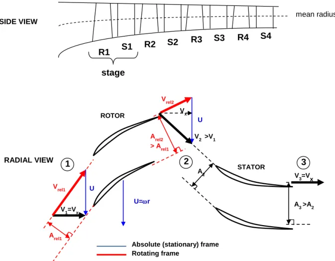
A typical compressor stage is composed of a moving blade row followed by a stationary blade row. Two main types of compressors exist as defined by the change in mean radius of the flow from inlet to exit. When this change is minimal, it is an axial compressor and when it is important it is usually a centrifugal compressor. As shown in Figure 1-2, a rotor (moving blade row) redirects the flow in the relative frame thus increasing both static pressure through normal flow area increase and stagnation (total) pressure by increasing the flow velocity in the circumferential direction in the absolute frame. A stator (stationary blade row) redirects the flow toward the axial direction thus converting the increased kinetic energy into static pressure rise. For a centrifugal

(19)

compressor, shown in Figure 1-3, the moving blade row is an impeller which adds a lot more rotation to the flow, compared to an axial rotor, due to the large radius change from inlet to exit. At the same time, the centrifugal force from the rotation ensures a larger static pressure rise across the impeller than that across an axial rotor. However, the need for the diffuser to turn the high swirling flow exiting the impeller both circumferentially and radially back toward the axial direction results in higher pressure losses than in a stator. As a result, a centrifugal compressor stage provides several times more pressure rise than an axial stage but generally suffers from lower adiabatic efficiency and larger frontal area. A more seldom used type of compressor is the mixed flow compressor, which is essentially an axial stage with a large radius change in the rotor, as illustrated in Figure 1-4. It combines the effect of the axial centrifugal compressor, giving performances somewhere in-between.

Figure 1-2: Axial compressor stage

R1 S1 R2 S2 R3 S3 R4 S4 mean radius stage U V₁=V_x U=r U V 2 >V1 V_x V_rel1 V rel2 A_rel1 A rel2 > A rel1 A 2 ROTOR STATOR A 3 >A2 V₃=V x

Absolute (stationary) frame Rotating frame

SIDE VIEW

(20)

Figure 1-3: Centrifugal compressor stage

Figure 1-4: Mixed flow compressor

rotor V 3 stator V 1 1 2 3 1 3 SIDE VIEW

(21)

The compressor is arguably the most difficult component to design in a gas turbine from an aerodynamic stand point because it is essentially forcing the flow to go against a positive pressure gradient, making the blades susceptible to boundary layer separation. As such, the stage pressure ratio is limited and it requires many stages to achieve a required pressure ratio, making it the longest component of a gas turbine engine. In an aircraft application, where the number of compressor stages should be held to a minimum to limit engine length and weight, a combination of axial and centrifugal stages as shown in Figure 1-5 can sometime be used, especially in smaller engines where the rotational stresses of the smaller impellers can be kept reasonable, to minimize the number of stages without sacrificing too much in efficiency.

Figure 1-5: Example of axial-centrifugal multi-stage compressor[2]

1.2 Aerodynamic Instabilities

Figure 1-6 shows a typical compressor map in which each speedline represents the pressure rise versus mass flow at one particular rotation speed. As the mass flow decreases along a speedline, the axial velocity in Figure 1-2 increases, resulting in higher flow incidence and flow turning in the rotor and stator which increases pressure rise but also total pressure losses from among other things larger boundary layer growth on the blade/end wall surfaces from larger pressure gradients inside the blade passages. The increase in losses may lead the pressure rise to turn over as illustrated in Figure 1-6. Eventually, the speedline reaches an aerodynamic stability limit called stall point or surge point beyond which for example the blade boundary layer may separate. The line linking the stall/surge points of different speedlines is referred to as the stall line or the surge line.

(22)

Figure 1-6: A schematic representation of a compressor map

At the stall/surge point, two types of aerodynamic instabilities can appear that are illustrated in Figure 1-7 for one particular speed. The first is rotating stall, which is characterized by the formation of a cell of velocity deficiency that rotates around the circumference at part of the rotor speed. By itself, rotating stall can cause a small drop in pressure rise (mild form) or a large drop in pressure rise (sever form) along the dashed line representing the combustor/turbine pressure drop characteristics intersecting the compressor speedline at the stall/surge point. However, in gas turbine applications, rotating stall usually triggers a much more severe instability called surge. Surge is an essentially axisymmetric flow oscillation across the entire gas turbine which in its most severe form (called deep surge), as illustrated in Figure 1-7, involves flow reversal across the compressor during part of the surge cycle. The link between rotating stall and surge can be intuitively understood as the inability of the compressor, once rotating stall occurs, to maintain the pressure inside the combustor leading to a partial discharge of the stored pressurized fluid and drop in combustor pressure until the compressor is able to pump flow anew, leading to

Surge point Design point Pressure Rise Mass Flow

(23)

the surge cycle. Surge usually leads to a sudden and dramatic drop in engine power and damages to the engine and as such must be avoided.

Figure 1-7: Aerodynamic instabilities for a compressor

1.3 Problem Definition

To avoid surge during engine operation, the design point of the compressor is placed away from the stall/surge point. As the engine accelerates or decelerates the compressor operates along a line called running line that intersects this point, as shown in Figure 1-6.The running line is set by a thermodynamic balance between the compressor combustor and turbine at the different operating speeds. For a particular gas turbine, this line can be set by the turbine design. The distance between the running line and stall/surge line is referred to as the surge margin. However, neither the surge line nor running line are fixed in an actual gas turbine engine. Engine inlet flow distortion and engine wear usually causes the surge line in Figure 1-6 to move to the right whereas rapid engine acceleration will make the running deviate to the left, both factors reducing surge margin and putting an engine at risk for surge during its operating life time. Furthermore, while the designer may try to incorporate adequate stall/surge margin, given the difficulty in accurately predicting the compressor stall point, the compressor must be mapped experimentally to find the actual surge line. Thus, it is inevitable that the gas turbine will be surged repeatedly

Pressure Rise

stall/surge pt. surge

rotating stall(alone)

(24)

during its development phase. As such, one must ensure during the design phase that the components will withstand the aerodynamic load brought about by a surge event and that the gas turbine would survive the flow oscillation in conditions of the cooling flow extracted inside the compressor.

As rotating stall is usually the trigger for surge, much of research on aerodynamic instabilities over the past few decades has focused on predicting rotating stall as in the work by Day [3] and suppressing its inception [4] to extend stall/surge margin. Relatively little research has been performed on surge. Some of this research have looked at analytically simulating the surge cycle for low-speed axial compressors as a whole, such as reference [5], while others more recent work focused on CFD simulations of compressors with final 3-D blade geometries as described in [6]. However, at the preliminary design phase of an engine, the three-dimensional compressor blade geometries are not yet defined. Instead, only the gas path and blade chord, thickness and inlet/exit angles at the mean radius along the gas path (meanline) and blade count are determined through rapid iterations using analytical models that rely on quasi-1-D flow physics and loss correlations to predict the compressor map (and turbine map) and by extension the engine performance. Yet, it is based on the results from the preliminary design phase that engine weight and performance specifications and component design objectives are set for the rest of the design, making this phase extremely important. Consequently, it is important to have an idea at this phase about the aerodynamically induced forces involved during surge for proper preliminary dimensioning of engine components. An estimate of oscillation frequency would also be useful for prevent resonance of certain components. Thus, there is a need for a method to predict, right from the preliminary design phase and even with order-of-magnitude accuracy in amplitude, the oscillations of flow parameters (mainly pressure, velocity/momentum and mass flow) at relevant points inside a multi-stage compressor required for calculating aerodynamics forces and cooling bleed mass flows during surge.

1.4 Objectives

The objective of this research is to develop and evaluate a rapid method to predict, within order of magnitude accuracy or better, the temporal variation during a surge cycle of flow properties at pertinent meridional locations along the meanline of a multi-stage axial or non-axial compressor. These locations could be the compressor inlet or exit or at locations between certain blade rows

(25)

where air extractions are taken or when flow properties are needed for a control volume analysis to calculate the aerodynamic forces on a blade row or on the shaft holding multiple compressor blade rows. This method is to be used in the preliminary phase when rapid design iterations are being carried out.

1.5 Thesis Outline

Following this introduction chapter, this remainder of the thesis is organized as follows:

Chapter 2 contains a literature review covering past research on compressor surge simulations to identify pertinent works that will contribute to the method developed in this project.

Chapter 3 presents the method proposed and the way in which it is implemented numerically for surge simulations. It also describes the axial and non-axial compressor geometries that will serve as test cases to evaluate the proposed method.

Chapter 4 presents the results of the method as applied to the studied geometries along with an assessment of the effectiveness of the method with regard to the objectives of the study.

Finally, Chapter 5 summarizes the main conclusions of this study and presents suggestions for future work.

(26)

CHAPTER 2 LITERATURE REVIEW

This chapter presents an overview of the state of the art in compressor surge simulations. This information will be highly useful for developing a method for predicting surge induced flow oscillations within multi-stage compressors according to the objective of the current research. The past works in this field can be placed under two categories, namely analytical methods and computational methods.

2.1 Analytical Methods

In the 1950s, Emmons et al. [7] were the first to identify the two compressor aerodynamic instabilities, namely rotating stall and surge, through experiments on different compressors. They stipulated that a compression system is dynamically unstable near the peak of the pressure rise/mass flow characteristic (speedline) as its slope becomes positive. They proposed a qualitative explanation for rotating stall based a rotating pattern of 2-D blade suction side boundary separation and used a Helmholtz resonator analogy for surge. In the latter case, the compressor/duct length and combustor volume were modelled as the pipe length and plenum volume to get a rough estimate of the oscillation frequency.

The next significant development in surge modelling only came about two decades later when Greitzer [5] proposed a lumped-parameter model to simulate surge in low-speed (incompressible) axial compressors. Recognizing that surge involves not just the compressor but other elements of the entire compression system, Greitzer modelled the main components of a gas turbine with discrete lumped elements, namely an actuator disk as the compressor, a plenum to model the combustor and a throttle as the turbine, as illustrated in Figure 2-1. The flow is incompressible in all components except in the plenum.

The compressor is modelled as an actuator disk that incorporates fluid inertia across which the instantaneous pressure rise is given by the steady pressure rise, obtained through the speedline at the given instantaneous mass flow from which is subtracted the inertia of the fluid across the compressor (and associated duct). The combustor is modelled as a plenum volume of stagnant compressible gas with spatially uniform properties whose pressure matches the exit pressure of the compressor and inlet pressure of the turbine. The compression/expansion process in the plenum is assumed to be isentropic. Finally, the turbine is simply treated as a throttle with a

(27)

quadratic relationship between pressure drop and mass flow that dumps the air into the same reservoir pressure as that at which the air enters the compressor. Thus, the total-to-static pressure rise across the compressor is the same as the static pressure drop across the turbine.

Figure 2-1: Schematic of Greitzer model [5]

Figure 2-2: Operating points from pressure matching between compressor and throttle (turbine)

The result of the pressure matching between the three components in the Greitzer model is illustrated in Figure 2-2, which shows the compressor speedline, with the stable part being the solid line and the unstable part (‘axisymmetric’ stall condition) the dashed line. The throttle characteristics (pressure drop versus mass flow) are shown as dotted lines for different throttle openings, each opening described by a constant value of KT. When the compressor is operated in

the stable region, the operating point represents the intersection of the stable part of the speedline

Pressure Rise Mass Flow positive flow reversed flow unstable speedline stable speedline throttle characteristics KT

(28)

for and the throttle characteristic, where the pressure matches for the same mass flow. As the throttle is closed (value of KT increased), the flow settles to a new stable operating point up the

speedline. However, beyond the last stable point, i.e. the stall/surge point, there is no longer an equilibrium point where pressure matches at the same mass flow across the compressor and turbine and the solution will go to a limit cycle (surge). The results from the Greitzer model compared well with experiments as shown in Figure 2-3.

Figure 2-3: Experimental validation of model by Greitzer[8]

In addition, Greitzer also proposed a non-dimensional parameter called B-parameter, as a similitude parameter for surge behavior among different compression systems. This parameter can according to him be used to predict whether a compression system will exhibit surge or remain in rotating stall. As defined in equation (2.1) the B parameter involves the compressor rotating speed (U), sound speed (a), annular area (A), length (L) and plenum volume (V).

B =

U 2a_𝑠

√

V

AL (2.1)

Based on theory and experimental data of a low-speed axial compressor with different plenum volumes, as presented in Figure 2-4, Greizer [8] showed that surge would only occur for B greater than 0.7 or 0.8. Thus an increase in plenum volume and/or rotation speed will tend to drive the system toward surge.

(29)

Figure 2-4: Onset of surge for different plenum volume[8]

Greitzer [8] showed two experimental cases, both presented in Figure 2-5, one with low speed and high plenum volume and the other with higher speed and lower plenum volume but with about the same value of the B parameter. One can see that the surge limit cycle is essentially the same justifying the claim of the B parameter as a similitude parameter.

Figure 2-5: Experimental results for two surge cycle with the same B parameter [8]

The Greitzer model has the advantages of simplicity, calculation speed and the capability to provide good results. However, it has certain notable drawbacks. First, it requires not only the stable part of the speedline but also the unstable part (which includes the negative flow region) as

(30)

shown by the dashed line in Figure 2-2, which is very hard to obtain either experimentally or even computationally and certainly not known at the preliminary design phase. Second, in treating the compressor as a single actuator disk, one cannot obtain the flow parameters inside of the compressor. Third, the role of the B parameter as a similitude parameter has been questioned by subsequent work. While Greitzer [8] showed similarity of the surge limit cycle in Figure 2-5 for the same B parameter, he did not compare the temporal variation of pressure and mass flow to show whether the oscillations have the same frequency. Works by other researchers [6, 9] later showed that the surge limit cycle shape on the compressor map can be the same for the same B parameter without the oscillation frequency being the same. Last but not least, due to the assumptions of axial flow and incompressibility, the model is limited to low-speed axial compressors. However, Hansen et al [10] demonstrated experimentally that the model seems to apply also be adapted to a centrifugal compressor although without proving it analytically. However, his results also showed that the critical B parameter value of 0.8 for surge does not apply in this case. Similarly, Day [11] also showed experimentally, on a low-speed axial compressor, that this critical B parameter value is not universal.

Nevertheless, the Greitzer model formed the basis for many subsequent analytical modelling works on compressor aerodynamic instabilities, most of which concentrated on prediction and suppression (through flow control) of rotating stall inception. These works started with those by Moore[12] and Moore and Greitzer [13, 14] who expanded lumped-parameter model to include the circumferential flow variation in order to capture rotating stall in low-speed axial compressors. Bonnaure [15] developed a two-dimensional compressible model in the axial multi-stages compression system that relied on loss and deviation correlations for each blade row. The model is used to predict the onset of stall but does not predict the surge cycle. Spakovszky [16] developed a new model to predict the radial effects on the compression system, but this model is suitable for control purposes and cannot be developed to predict the surge cycle. Weigl [17] introduced another model developed from the Bonnaure [15] work, but which was also used for rotating stall inception.

More recently, Morini et al. [18] proposed a model based on a modular approach in which each component (inlet or exit plenum, duct, compressor) can be discretized into multiple elements instead of one lumped parameter and the one-dimensional equations of conservation of mass, momentum and energy equations can be solved using the finite difference method. In principle,

(31)

this modular approach should allow for putting together complex combinations of the elements of a compression system and even include heat transfer through the energy equation. However, the authors only solved for a standard volume-duct-compressor-duct-volume combination in which the compressor seems to have been treated in one lumped-parameter approach through the speedline as with the Greitzer model. Their placement of the emphasis on solving the equations in the ducts is not really relevant in an aero-engine where un-bladed ducts are kept to a minimum.

2.2 Computational Methods

The computational methods for surge simulations can be divided into two types, quasi-1D and 3D CFD. The quasi-1D computational methods started with the DYNTECC model of the compression system by Hale and Davis [19]. This model consists of discretizing the entire gas path of the compression system into elemental control volumes across which the 1-D conservation equations are applied along with source terms to account for the effects of blade forces, shaft work, mass bleed and heat transfer. These source terms must be determined from a complete set of stage pressure rise and temperature rise characteristics. The conservation equations are then solved through a finite difference numerical technique. Cousins [20] applied the DYNTECC model to simulate surge in an axial-centrifugal compressor. Garrard [21] later extended the DYNTECC model by incorporating modelling of the combustor and turbine to produce the ATEC model that can simulate the entire gas turbine. More recently, Du and Leonard [9] applied a similar method as the DYNTECC model in which the gas path of a compression system is discretized and the adapted 1D Euler equations are applied with source terms estimated from calculating the velocity triangles for each blade row and loss and blade deviation correlations. The 1D approaches above give good results in terms of simulating the surge cycle and would allow for the extraction of flow information inside the compressor during surge. However, they involve some preparation work in extracting the source terms and in obtaining a mesh independent solution.

With the increase in computational capabilities in recent years, a full 3-D computational approach has been proposed by several researchers. Niazi [22] simulated surge in an axial compressor with CFD using an unsteady RANS CFD research code. A full-annulus isolated compressor rotor was meshed and the effect of the downstream components was simulated through a dynamic boundary condition applied at the exit of the computational domain that gives the variation of the

(32)

pressure inside a plenum through an analytical equation. However, the turbine was not properly modelled in this equation as a simple constant mass flow rate was imposed at the plenum exit. The predicted temporal variations of pressure rise and flow coefficient are qualitatively reasonable but somewhat noisy. However, the results remain questionable due to the non-physical constant exit mass flow condition for the plenum.

Guo et al. [23] later applied the approach of Niazi [22] to simulate surge for an impeller using the RANS model of the commercial CFD code ANSYS CFX. In doing so, they used the same constant exit mass flow condition for the plenum model. Some of their results were highly irregular with non-repeatable surge cycles.

Vahadati et al. [24] carried out CFD simulations of surge in an eight-stage axial compressor by meshing only one blade passage per blade row. Instead of a plenum and valve, they included a meshed converging nozzle in the computational domain downstream of the compressor. The use of only one blade row per blade passage is an ingenious way of taking advantage of the essentially one-dimensional nature of surge while reducing computational requirements. However, the drawbacks of this work are the need to modify the nozzle shaped and remesh for each simulated point up the speedline in search for the stall/surge point and the challenge in correctly representing combustor and turbine properties with the nozzle on a quantitative basis. Finally, Dumas [6] combined the best features of the above approaches in a method for simulating surge in any multi-stage compressor. As illustrated in Figure 2-6, his approach essentially consists of using single blade passage multi-stage RANS CFD simulations of the compressor with ANSYS CFX, as done by Vahadati et al. [24], but for which a dynamic exit boundary conditions was applied at the compressor computational domain exit, similar to the strategy proposed by Niazi [22]. However, unlike Niazi [22], to analytical equation for the dynamic exit boundary condition was obtained using the same modelling approach as Greitzer in which the turbine was represented as a valve with a quadratic pressure-mass flow relationship rather than a constant mass flow condition. This method was used to simulate surge on three compressor geometries: a low-speed three-stage axial compressor for which surge data exists; a low-speed axial-centrifugal compressor with small compressibility effects composed of the previous three-stage axial compressor matched to an impeller with a vaneless diffuser; and a high-speed mixed-flow-centrifugal compressor in which the compressibility effects are

(33)

important. In spite of very limited test data for validation, Dumas [6] showed that the simulations worked well though a good match with the measured surge cycle for the low-speed there-stage axial compressor as shown in Figure 2-7.

Figure 2-6: Illustration of the methodology used by Dumas [6]

Figure 2-7: Comparison of simulated surge cycle of low-speed axial compressor by Dumas with test data[6]

(34)

The full 3D RANS CFD approach, culminating in the work by Dumas [6], can deliver all local flow information at any point inside the compressor during surge to a greater extent than any approach so far without requiring any empiricism beyond the turbulence models and numerical issues associated with CFD simulations. However, this approach requires knowledge of the three-dimensional blade geometries, preparation work on mesh dependency studies, as well as relatively significant computational resources and time.

(35)

CHAPTER 3 METHODOLOGY

This chapter describes the methodology taken to address the objectives of this project starting with a qualitative description of the general strategy, followed by the setup of equations and verification of applicability to non-axial compressors. The chapter concludes with a description of three compressor geometries to be used for evaluation of the model and the procedure for running the model.

3.1 General Strategy

Chapter 2 provided an overview of the different strategies taken in the past to simulate surge, ranging from analytical models to full-scale 3D RANS CFD simulations. The objective of this project is to provide a fast method to predict, within order of magnitude accuracy or better, the temporal variation of flow properties at relevant location in a multi-stage compressor during surge, to be used during the preliminary design stage. Consequently, the 3-D RANS CFD approach cannot be considered, not only because it is time-consuming, but also because the full blade geometries are not available at the early design stage. Among lower-fidelity models, the quasi-1D models would be a good option; however, they do require work for extracting source terms from the compressor characteristics and for discretizing the compression domain, which is not ideal at the preliminary design phase where there is a need for rapid turn-around time during preliminary design iterations. As a result the strategy chosen was to develop a method based on the Greitzer model, but with the addition of a new element to allow for extracting flow property variations at points of interest inside the compressor.

The proposed strategy consists of using the Greitzer model approach to predict the surge cycle of the entire compressor and then deduct from the compressor exit pressure the unsteady pressure rise associated with the compressor section between the desired location and the compressor exit. The unsteady pressure rise of the last section would comprise the steady pressure rise and the fluid inertia effects associated with this section. With the incompressibility assumption in the Greitzer model, the flow oscillation at the desired section can be simply deduced from the local cross flow area and mass flow conservation. This strategy is illustrated in Figure 3-1 for a three stage compressor in which the inquiry plane lies between the second and third stage. This is essentially the new contribution of this work.

(36)

Figure 3-1: Example of proposed surge simulation strategy applied to a three-stage axial compressor

The advantage of this method is that it is simple and very fast, not only in run calculation time but also in preparation time since it would directly use the speedline (for the whole compressor and relevant sections) output from the meanline code at the preliminary design stage without any need to extract source terms, nor loss/deviation correlations that are implicit in the meanline code. However, the Geitzer approach presents two drawbacks for applications to generic multi-stage compressor. First, it was meant only for axial compressors. Nevertheless, Hansen et al. [10] did suggest, through comparison with experimental data, that the model can be applied to a centrifugal compressor and this will be verified analytically. Second, the model assumes incompressible flow inside the compressor. However, compressibility would reduce the amplitude of pressure oscillations through absorption of some of the energy in compression of the fluid. As such the incompressible model with air density taken at the inlet value should provide a conservative estimate of pressure oscillation amplitudes that may be adequate for an order-of-magnitude prediction accuracy requirement, which can be assessed through case studies.

While the Greitzer approach is chosen, the improved version of the model called the Moore-Greitzer model as described by Moore and Moore-Greitzer [13] is chosen as the surge simulation strategy for the entire compressor. This model adds the circumferential dimension to the Greizer model enabling it to predict both surge and rotating stall. While rotating stall is not the focus of the present work, the Moore-Greitzer formulation provides more adequate and detailed representation of the compressor blade rows in the calculation of the inertia effects, which is

Greitzer model applied to 3A Pressure at 3A exit plane Unsteady pressure rise of 1A

(37)

important in this case to extract flow information within the compressor. At the same time, it also gives the final method the potential capability of simulating rotating stall.

3.2 Model Formulation

The equations of the Moore-Greitzer [13] model are derived for the basic compression configuration laid out in Figure 3-2, which is composed of an inlet duct of length (LI), a

multi-stage compressor, an exit duct of length (LE), a plenum and a throttle valve. With the exception of

the plenum, the flow in the rest of the system is treated as incompressible. It is assumed that the two ducts are lossless and that the turbine dumps air into an exit static pressure equal to the total pressure of the air entering the compressor. This is usually the case for a gas turbine engine where the exhaust static pressure and inlet total pressure are at the value of the atmospheric pressure.

Figure 3-2: Schematic of compression system[13]

3.2.1 Compressor and Ducts

The instantaneous total-to-static pressure rise (Pout – PT,in) across the duct-compressor-duct

system can be taken as the steady-state total-to-static pressure rise across the compressor (Pout –

PT,in)ss minus the static pressure drop associated with the inertia effect Pinertia from acceleration

of the fluid in the ducts and compressor blade passages as shown in equation (3.1).

𝑃_𝑜𝑢𝑡− 𝑃_{𝑇,𝑖𝑛} = (𝑃_𝑜𝑢𝑡− 𝑃_{𝑇,𝑖𝑛})_𝑠𝑠 − ∆𝑃_{𝑖𝑛𝑒𝑟𝑡𝑖𝑎} (3.1)

The inertia term can be calculated by considering the approximate blade geometries and duct lengths and knowing from the unsteady Bernoulli’s equation that the static pressure difference

LI LE

Lc

(38)

due to unsteadiness between two points along a streamline is given by L(dvs/dt), where , L and

(dvs/dt) are the respectively, the density, streamline length and time rate of change of streamwise

velocity in the relative frame. As such, for a turbomachinery blade passage with a blade chord b and stagger angle  and a meridional velocity Cm as illustrated in Figure 3-3, the unsteady

pressure drop due to inertia effect are given by equations (3.2) and (3.3) for a stator and a rotor, respectively. The multiplier k is a correction factor for b to account for the distances between blade rows and curvature effects to blade passage curvature (the latter neglected in this study). In the case of the rotor, U is the circumferential rotational speed at the compressor inlet mean radius. In a similar manner, equation (3.4) gives the inertia effect for a duct with duct length Lduct

in which the flow has a swirl angle  (which is usually zero as for the cases studied in this work).

Figure 3-3: Blade passage approximation for calculating inertia effect

∆𝑃_{𝑖𝑛𝑒𝑟𝑡𝑖𝑎, 𝑠𝑡𝑎𝑡𝑜𝑟} = 𝜌𝑘𝑏𝐷(𝐶𝑚/𝑐𝑜𝑠𝛾) 𝐷𝑡 = 𝜌𝑘𝑏 cos 𝛾 𝜕𝐶𝑚 𝜕𝑡 (3.2) ∆𝑃_{𝑖𝑛𝑒𝑟𝑡𝑖𝑎, 𝑟𝑜𝑡𝑜𝑟} = 𝜌𝑘𝑏𝐷(𝐶𝑚/𝑐𝑜𝑠𝛾) 𝐷𝑡 = 𝜌𝑘𝑏 cos 𝛾( 𝜕𝐶𝑚 𝜕𝑡 + 𝜕𝐶𝑚 𝜕𝜃 𝑑𝜃𝑟𝑜𝑡𝑜𝑟 𝑑𝑡 ) = 𝜌𝑘𝑏 cos 𝛾( 𝜕𝐶𝑚 𝜕𝑡 + 𝜕𝐶𝑚 𝜕𝜃 𝑈 𝑅) (3.3) ∆𝑃𝑖𝑛𝑒𝑟𝑡𝑖𝑎, 𝑑𝑢𝑐𝑡 = 𝜌𝐿𝑑𝑢𝑐𝑡𝐷(𝐶𝑚_𝐷𝑡/𝑐𝑜𝑠𝛼)= 𝜌𝐿_{cos 𝛼}𝑑𝑢𝑐𝑡𝜕𝐶_𝜕𝑡𝑚 (3.4)

Incorporating equations (3.2) through (3.4) for all blades rows and ducts into equation (3.1) gives equation (3.5).

𝑃𝑜𝑢𝑡− 𝑃𝑡,𝑖𝑛= (𝑃𝑜𝑢𝑡 − 𝑃𝑡,𝑖𝑛)_𝑠𝑠− [∑𝑁𝑟𝑜𝑡𝑜𝑟1 _{cos 𝛾}𝜌𝑘𝑏 −∑𝑁𝑠𝑡𝑎𝑡𝑜𝑟1 _{cos 𝛾}𝜌𝑘𝑏 − ∑𝑁𝑑𝑢𝑐𝑡𝑠1 𝜌𝐿_{cos 𝛼}𝑑𝑢𝑐𝑡]𝜕𝐶_𝜕𝑡𝑚−

[∑𝑁𝑟𝑜𝑡𝑜𝑟_{cos 𝛾}𝜌𝑘𝑏

1 ]𝜕𝐶_𝜕𝜃𝑚𝑈_𝑅 (3.5)

(39)

Non-dimensionalizing equation (3.5) with the four non-dimensional parameters defined below and assuming zero swirl in the inlet and exit ducts (= 0) gives equation (3.6), in which c ( ) is

the steady-state axisymmetric total-to-static compressor pressure rise characteristic (speedline). 1. 𝜑≡𝐶_𝑈𝑚 Dimensionless mass flow coefficient

2. 𝛹≡𝑃𝑜𝑢𝑡−𝑃𝑇,𝑖𝑛

𝜌𝑈2 Dimensionless total-to-static pressure-rise coefficient

3. 𝑙 ≡_𝑅𝐿 Dimensionless length

4. 𝜉 ≡ 𝑈_𝑅𝑡 Dimensionless time

𝛹 = 𝛹𝑐(𝜑) − (𝑙𝐼+ 𝑙𝑅 + 𝑙𝑆+ 𝑙𝐸)𝜕𝜑_𝜕𝜉− 𝑙𝑅𝜕𝜑_𝜕𝜃 (3.6)

, where 𝑙𝑅 ≡ ∑𝑁𝑟𝑜𝑡𝑜𝑟1 _{𝑅𝑐𝑜𝑠 𝛾}𝑘𝑏 ; 𝑙𝑆 ≡ ∑𝑁𝑠𝑡𝑎𝑡𝑜𝑟1 _{𝑅cos 𝛾}𝑘𝑏 ; 𝑙𝐼 ≡ 𝐿_𝑅𝐼 ;𝑙𝐸 ≡ 𝐿_𝑅𝐸

Next, to introduce the circumferential perturbation associated with rotating stall, as detailed in Moore and Greitzer [13] and summarized here, the flow coefficient  is split into an axisymmetric part  that accounts for steady-state operation plus axisymmetric (surge-type) perturbations and a circumferentially varying part g (meridional direction) and h (circumferential direction) for rotating stall-type perturbations, as shown in equation (3.7), where g and h integrate to zero over the circumference and can be obtained from a perturbation potential 𝜙̃′(𝜉, 𝜂, 𝜃) evaluated at the compressor inlet (station 0 in Figure 3-1). This potential exists through an irrotational flow assumption for the upstream duct. The variable  is the axial distance, non-dimensionalized by R, with the origin at station 0.

𝜑(𝜉, 𝜃) = 𝛷(𝜉) + 𝑔(𝜉, 𝜃); (𝜉, 𝜃) = (𝜙̃𝜂′)₀ ; ℎ(𝜉, 𝜃) = (𝜙̃𝜃′)₀ (3.7)

Incorporating equation (3.7) into (3.6) and given that the perturbations g and h apply only to the compressor, one obtains equation (3.8). The term 𝑚(𝜙̃_𝜉′)

0 accounts for pressure perturbations in

the exit duct in which the flow is assumed rotational with very small pressure perturbations. The value of m is 1 for a short exit duct and 2 for a long exit duct.

(40)

𝛹 = 𝛹𝑐(𝛷 + (𝜙̃𝜂′)₀) − (𝑙𝐼+ 𝑙𝑅 + 𝑙𝑆+ 𝑙𝐸)𝑑𝛷_𝑑𝜉 − 𝑚(𝜙̃𝜉′)₀− 𝑙𝑅(𝜙̃𝜉𝜂′ + 𝜙̃𝜃𝜂′ )₀− 𝑙𝑆(𝜙̃𝜉𝜂′ )₀

(3.8) To remove the derivative in  Moore and Greitzer [13] introduced a simplification based the fact that the perturbation g is circumferentially periodic, and keeping only the first term of the Fourier series solution for 𝜙̃𝜂𝜂′ + 𝜙̃𝜃𝜃′ = 0 which results in (𝜙̃𝜂′)₀ = −(𝜙̃𝜃𝜃′ )₀ allowing one to define a

perturbation function Y(,)(𝜙̃′)₀which gives (𝜙̃_𝜂′)

0 = −𝑌𝜃𝜃. Thus, equation (3.8) becomes:

𝛹 = 𝛹_𝑐(𝛷 − 𝑌_𝜃𝜃) − (𝑙_𝐼+ 𝑙_𝑅 + 𝑙_𝑆+ 𝑙_𝐸)𝑑𝛷

𝑑𝜉 − 𝑚𝑌𝜉+ 𝑙𝑅(𝑌𝜉𝜃𝜃+ 𝑌𝜃𝜃𝜃) + 𝑙𝑆𝑌𝜉𝜃𝜃 (3.9)

Finally, the inertia terms for the blade rows are combined through the definition of an average inertia parameter  defined as in equation (3.10) which allows for the combination of the terms 𝑙𝑅

and 𝑙_𝑆 into a single term 1/a where a is defined as in equation (3.11) so that equations (3.9) simplifies to equation (3.12). 𝜏 ≡2(𝑙𝑅+𝑙𝑆)𝑅 𝑈𝑁𝑠𝑡𝑎𝑔𝑒𝑠 (3.10) 𝑎 ≡_{𝑈𝜏𝑁𝑠𝑡𝑎𝑔𝑒𝑠}𝑅 (3.11) 𝛹(𝜉) = 𝛹𝑐(𝛷(𝜉) − 𝑌𝜃𝜃) − 𝑙𝑐𝑑𝛷_𝑑𝜉 − 𝑚𝑌𝜉 +_2𝑎1 (2𝑌𝜉𝜃𝜃+ 𝑌𝜃𝜃𝜃) (3.12) , where 𝑙_𝑐 ≡ 𝑙_𝐼+1_𝑎+ 𝑙_𝐸

The last equation which gives the pressure rise from the gas turbine engine inlet to the end of the stator of the plenum is obtained by integrating the equation (3.12) over the circumference, considering that ∫ 𝑌(𝜉, 𝜃)𝑑𝜃 = 0₀2𝜋 , which results in equation (3.13)

𝛹(𝜉) = _2𝜋1 ∫ 𝜓₀2𝜋 𝑐(𝛷(𝜉) − 𝑌𝜃𝜃)𝑑𝜃 − 𝑙𝑐𝑑𝛷_𝑑𝜉 (3.13)

The fine details of the above derivations and of the definitions of the different parameters used can be found in references [12, 13].

(41)

3.2.2 Plenum and Throttle

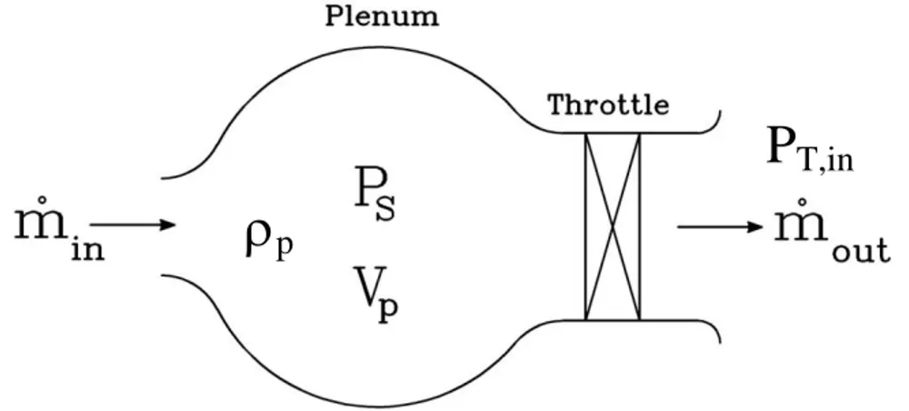
From the lumped parameter approach of Greitzer, the air in the plenum is assumed to be an ideal gas at rest with spatially uniform properties as illustrated in Figure 3-4. The compression/expansion process in the plenum is assumed to be isentropic.

Figure 3-4 : Modelling of plenum and throttle Mass conservation (𝑚̇) applied to the plenum results in equation (3.14)

𝑚̇𝑖𝑛− 𝑚̇𝑜𝑢𝑡 = 𝑑(𝜌_𝑑𝑡𝑝𝑉𝑝)= 𝑉𝑝𝑑(𝜌_𝑑𝑡𝑝) (3.14)

With the ideal gas law 𝑃 = ρR̃T, where R̃= 287 𝐽. 𝐾𝑔−1. 𝐾−1 is the specific gas constant for air and an isentropic process 𝑃1−𝛾𝑇𝛾 = 𝐶𝑜𝑛𝑠𝑡𝑎𝑛𝑡, where γ is the specific heat ratio, one obtains equation (3.15), where 𝑎_𝑠 is the speed of sound in air. Combining equations (3.14) and (3.15) results in equation (3.16) which describes the time variation of the plenum pressure 𝑃_𝑆 with respect to the mass flow at its inlet and outlet.

𝑑(𝜌𝑝) 𝑑𝑡 = 1 R̃𝛾𝑇_𝑝 𝑑𝑃_𝑆 𝑑𝑡 = 1 𝑎𝑠2 𝑑𝑃_𝑆 𝑑𝑡 (3.15) 𝑑𝑃_𝑆 𝑑𝑡 = 𝑎_𝑠2 𝑉𝑝 (𝑚̇𝑖𝑛− 𝑚̇𝑜𝑢𝑡) (3.16)

Considering that PS is the same as the pressure exiting the downstream duct of the compressor,

that 𝑚̇_𝑖𝑛 = 𝑚̇_{𝑐𝑜𝑚𝑝𝑟𝑒𝑠𝑠𝑜𝑟} = 𝜌𝐶_𝑚𝑆_𝑐, where Sc is the compressor cross-sectional area and that the



p

(42)

pressure drop across the throttle follows the quadratic relation laid out in equation (3.17), equation (3.16) reduces to its non-dimensional form to equation (3.18),

𝛥𝑃_{𝑡ℎ𝑟𝑜𝑡𝑡𝑙𝑒} = 1₂𝐾_𝑡𝑚̇_𝑜𝑢𝑡2 = 𝑃_𝑆− 𝑃_{𝑇,𝑖𝑛} (3.17) 𝜕𝛹 𝜕𝜉 = 1 4𝐵2_𝑙 𝑐(𝛷(𝜉) − √ 2𝛹(𝜉) 𝐾_𝑡 ) (3.18) , where 𝐵 =_2∗𝑎𝑈 𝑠√ 𝑉𝑝

𝑆𝑐∗𝐿𝑐 is the Greitzer B parameter with 𝛹 and 𝛷 being, respectively, the

instantaneous total-to-static pressure rise coefficient and flow coefficient of the compressor-ducts system from equation (3.13).

3.2.3 Surge Simulation

Equations (3.12), (3.13) and (3.18) describe the non-linear behavior of the system for aerodynamic instabilities. In this case they were solved for the surge cycle of the entire compressor using the Galerkin procedure and MATLAB-Simulink according to the method described in Appendix A.

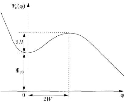
The model setup requires the use of a polynomial approximation for the full speedline. The format used by Moore and Greitzer [13] is a cubic polynomial described by equation (3.19), where the ψ_c0, H, and W parameters are shown in Figure 3-5. It is noted that the local flow coefficient in equation 3.19, φ = (𝛷 − 𝑌_𝜃𝜃), includes the term−𝑌_𝜃𝜃.

𝛹_𝑐(φ) = 𝛹_𝑐0+ 𝐻[1 +3₂(_𝑊φ− 1) −1₂(_𝑊φ − 1)3] (3.19) This cubic polynomial was chosen by Moore and Greitzer [13] based on the works by Koff [25, 26], which found this format to best match the full measured speedline in a low-speed multi-stage axial compressor. In the absence of a better alternative, this cubic speedline model is chosen for this study whose simulations will provide indications of the applicability of the speedline format to other compressors, in particular when unstable part of the characteristic is not known.

(43)

Figure 3-5: Notation used in definition of (axisymmetric) compressor characteristics

3.2.4 Surge Information Inside the Compressor

To obtain the pressure oscillation at a point between two blade rows inside a compressor such as shown in Figure 3-6, the static to static pressure rise 𝜓_{𝑆𝑆−𝑠𝑒𝑐𝑡𝑖𝑜𝑛2} and inertia effects ∆𝑃_{𝑖𝑛𝑒𝑟𝑡𝑖𝑎, 𝑠𝑒𝑐𝑡𝑖𝑜𝑛2} are simply deducted from the pressure rise 𝛹(𝜉) and flow coefficient 𝛷(𝜉) for the entire compressor (solved using the procedure described in Section 3.2.3 and Appendix A), as shown in equation (3.20).

Figure 3-6: Calculation of pressure at inquiry location inside compressor 𝛹_𝑐(φ) φ Section1 Section 2 𝛹(𝜉) 𝜓𝑆𝑆−𝑠𝑒𝑐𝑡𝑖𝑜𝑛2(𝛷(𝜉)) ∆𝑃𝑖𝑛𝑒𝑟𝑡𝑖𝑎, 𝑠𝑒𝑐𝑡𝑖𝑜𝑛2 inquiry location

(44)

𝛹(𝜉)Desired location= 𝛹(𝜉) − 𝜓𝑆𝑆, 𝑠𝑒𝑐𝑡𝑖𝑜𝑛2(𝛷(𝜉)) + ∆𝑃𝑖𝑛𝑒𝑟𝑡𝑖𝑎, 𝑠𝑒𝑐𝑡𝑖𝑜𝑛2 (3.20)

The static pressure rise characteristic 𝜓𝑆𝑆−𝑠𝑒𝑐𝑡𝑖𝑜𝑛2 can easily be produced by the meanline code

used during the preliminary aero-engine design phase and the inertia effect for section 2 can be calculated as in equations (3.2) through (3.4) for the blade rows and ducts located in section 2. This calculation was simply carried out in MS Excel.

It is noted that the incompressible flow assumption through the compressor means that the flow oscillations inside the compressor are in phase with that of the entire compressor. However, this may not be far from the actual surge physics. Indeed, the time scale associated with the low-frequency surge oscillation is much longer than the acoustictraveling time across the compressor. Thus, the flow fluctuations associated with surge at different points inside the compressor would essentially be in phase.

3.3 Analytical Model Assessment for Non-Axial Compressors

While the experimental assessment of the Greitzer surge model by Hansen et al. [17] suggested that this approach should work also for a non-axial compressor, it would be interesting to prove it analytically. The main element of this approach is the inertia effect. Let’s consider the static pressure rise of flow through a centrifugal compressor impeller as illustrated in Figure 3-7. The Euler equation in the relative (rotating) frame, which includes a centrifugal and a coriolis terms to account for the pseudo-forces due to rotational speed , is given in vector form by equation (3.21) and along the relative streamline by equation (3.22), with w and 𝑊⃗⃗⃗ being the relative velocity magnitude and vector, respectively. Integrating equation (3.22) along a relative streamline going from station 1 (l=0) to station 2 (l=L) located at a higher radius results in equation (3.23), which gives the instantaneous pressure difference between the two stations.

(45)

Figure 3-7: Velocity triangle at the impeller tip 𝜌𝐷𝑤_𝐷𝑡⃗⃗ = −1₂ 𝛻 (𝑝 −1₂𝜌𝛺2_𝑟2_{) − 2 𝛺⃗ ×𝑤}_⃗⃗ _(3.21) 𝜌𝜕𝑤_𝜕𝑡 + 𝜌𝑤𝜕𝑤_𝜕𝑙 = −𝑑𝑝_𝑑𝑙+ 𝛺2_𝑟𝑑𝑟 𝑑𝑙− 2𝜌𝛺⃗ × 𝑤⃗⃗ (3.22) 𝑃₂ − 𝑃₁ =1₂𝜌(𝑤₁2_{− 𝑤} 22) −1₂𝛺2(𝑟12− 𝑟22) − 2𝜌 ∫ 𝛺⃗ × 𝑤₀𝐿 ⃗⃗ 𝑑𝑙− 𝜌 ∫₀𝐿𝜕𝑤_𝜕𝑡𝑑𝑙 (3.23)

Equation (3.23) shows that the inertial effect term(∫₀𝐿∂w_∂t d𝑙), which represents the central effect of unsteadiness through the compressor in the Greitzer modelling approach, is independent of radius change, and is thus no different than for an axial rotor. This means that the Greitzer surge model should work in non-axial geometries with non-negligible radius change.

3.4 Compressor Geometries for Model Assessment

As test data for surge are rare, the proposed surge simulation technique was assessed with the three compressor geometries used by Dumas [6] to allow assessment versus CFD data, when test data are not available. The first is a low-speed (incompressible) three stage axial geometry for which some test data are available as well as interstage data from Dumas’ CFD simulations. The second compressor is a low-speed axial-centrifugal geometry, with very little compressibility effect. The last geometry is a high-speed industrial compressor composed of a mixed flow stage, and a centrifugal stage, where compressibility effects are important.

(46)

3.4.1 Low-Speed Axial Compressor

The first study focuses on a three-stage low-speed axial compressor in a rig located at the Massachusetts Institute of Technology Gas Turbine Laboratory (MIT-GTL), henceforth referred to as the MIT-GTL LS3 compressor. It incorporates an IGV (Inlet Guide Vanes) placed upstream of the first rotor. Figure 3.8 taken from Gamache [27] provide an overview of the position and shape of the blade rows and main instrumentation layout. The hub and shroud diameters are constant at 536 and 610 mm, respectively. The compressor has a nominal length of 0.67 m, while the lengths of the inlet and exit ducts are 0.86 m and 0.44 m, respectively, giving a total length (Lc) of 1.97 m. The compressor rig was adapted by Protz [28] to study surge and its suppression

via active control. As illustrated in Figure 3-8, the compressor dumps air into a large plenum of 9.66 m³ in volume (to provide for a B parameter of 1), at the exit of which is a throttle valve. Downstream of this valve is a large duct that contains flow straighteners and an orifice plate for mass flow measurements as well as an exhaust fan. This fan had been used to force air in the reversed direction to obtain the reverse flow pressure rise characteristics of in the compressor [29]. This fan, however, was not operational during the surge experiments conducted by Protz[28].

The surge experiments by Protz [28] were carried out at 2600 rpm, giving a mean circumferential velocity (U) of 78 m/s. The measured surge cycle is shown in Figure 3-10 (data for B=1.02).

(47)

Figure 3-8: Schematic representation of the positions of the compressor blades and measurements of points for the MIT-GTL LS3 compressor [27]

(48)

Figure 3-10: Surge cycle captured by Protz for the MIT GTL LS3 [28]

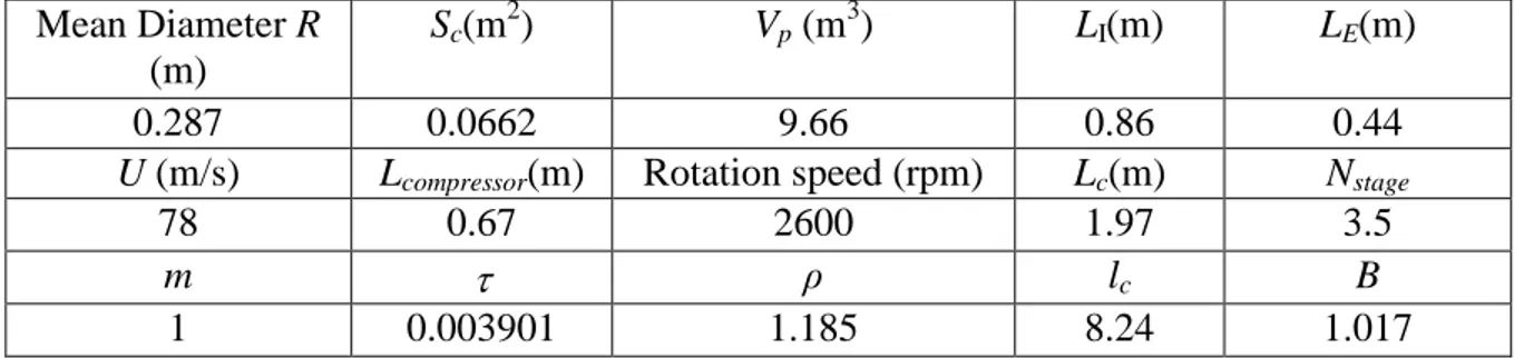
The meanline blade geometries and inter-stage distances were obtained from published works on this compressor [27, 28, 30] and the resulting modelled blade rows and dimensions used for the surge simulation modelling is illustrated in Figure 3-11. The inlet flow conditions were taken as standard atmospheric conditions. The resulting quantitative parameters used in the model is given in Table 3.1. The details of the calculation of the inertia parameter  for this compressor and the next compressor are provided in Appendix B. This compressor has surge test data for the compressor as a whole and CFD data for pressure oscillations between the second and third stage from Dumas [6] .