UNIVERSITÉ DE MONTRÉAL
ENHANCING THE GASOLINE VEHICLES’ CO2 EMISSIONS ESTIMATION IN MONTREAL
PEGAH NOURI
DÉPARTEMENT DES GÉNIES CIVIL, GÉOLOGIQUE ET DES MINES ÉCOLE POLYTECHNIQUE DE MONTRÉAL
THÈSE PRÉSENTÉE EN VUE DE L’OBTENTION DU DIPLÔME DE PHILOSOPIAE DOCTOR
(GÉNIE CIVIL) DÉCEMBRE 2015
UNIVERSITÉ DE MONTRÉAL
ÉCOLE POLYTECHNIQUE DE MONTRÉAL
Cette thèse intitulée :
ENHANCING THE GASOLINE VEHICLES’ CO2 EMISSIONS ESTIMATION IN MONTREAL
présentée par : NOURI Pegah
en vue de l’obtention du diplôme de : Philosophiae Doctor a été dûment acceptée par le jury d’examen constitué de :
M. CHAPLEAU Robert, Ph. D., président
Mme MORENCY Catherine, Ph. D., membre et directrice de recherche M. TRÉPANIER Martin, Ph. D., membre
ACKNOWLEDGEMENTS
I would like to express my sincere gratitude to my supervisor prof. Catherine Morency whose expertise, guidance and generous support made it possible for me to fulfil this research. It was a pleasure to be a part of Chaire Mobilité.
I would also wish to acknowledge the contribution and financial support of the four partners of the Mobilité research Chair: City of Montreal, Quebec Ministry of transportation, Montreal metropolitan agency and the Montreal transit authority, as well as Communauto that facilitated the data collection.
RÉSUMÉ
Les changements climatiques sont devenus l’un des enjeux environnementaux principaux des dernières années, les émissions de gaz à effet de serre (GES) étant pointées du doigt comme principal coupable. Globalement, les décideurs des politiques tentent depuis un certain temps de réduire les émissions des GES à travers diverses mesures et politiques. Considérant qu’en Amérique du Nord, le domaine du transport compte pour 30% des émissions totales, il est devenu le centre d’attention pour les initiatives de réduction des émissions de GES.
La première étape à suivre pour implémenter une politique ou une stratégie nouvelle est d’estimer son impact potentiel sur les émissions de GES ; à cette fin, l’utilisation des modèles d’émissions est essentielle. Depuis les années 70, plusieurs chercheurs ont développé des modèles d’émissions variés, atteignant une apogée lors des années 80. Les modèles d’émissions ont évolué depuis à travers plusieurs mises à jour, mais il y a encore de la place à l’amélioration. Puisque ces modèles sont extrêmement sensibles aux variations des données utilisées et aux méthodes de calibration, ne pas utiliser des bases de données précises ou effectuer une calibration fautive peut provoquer des estimations erronées.
Gardant cela en perspective, l’objectif principal de cette recherché est de contribuer à l’amélioration des modèles d’estimation des émissions. Pour se faire, trois objectifs ont été identifiés : le premier objectif spécifique est de fournir une revue des modèles disponibles et d’évaluer l’impact des divers facteurs sur les émissions. Le deuxième objectif spécifique est de comprendre et d’évaluer le modèle principal d’évaluation d’émission au Québec et d’identifier les variables qui sont les plus sensibles et qui peuvent le plus affecter les estimations. Le dernier objectif spécifique est d’améliorer la méthodologie pour développer les cycles de conduite utilisés dans les modèles d’émissions.
Afin d’atteindre ces objectifs, nous dédions le premier chapitre à discuter du sujet des changements climatiques et du domaine des transports en détail, avant d’aborder une introduction aux stratégies et politiques principales visant à réduire les émissions provenant du transport. Dans le deuxième chapitre, une revue détaillée des études disponibles sur le calcul, l’estimation et la représentation des émissions est fournie. Dans ce chapitre, le concept des cycles de conduite est également discuté, un facteur qui a été le centre d’attention dans les analyses d’émissions en raison de son impact significatif sur les émissions et de sa complexité de représentation.
Pour parvenir à nos objectifs, divers ensembles de données étaient nécessaires à l’analyse. Quelques-uns étaient déjà disponibles ; par contre, l’ensemble de données principal à cette étude, les données liées à l’utilisation du véhicule, a dû être collecté. Tous les ensembles de données et le processus de collection des données sont décrits dans le chapitre 3.
Pour le premier objectif spécifique, basé sur les modèles d’émissions qui sont présents dans la revue littéraire, une analyse de la sensibilité des facteurs est menée dans le quatrième chapitre. Cette analyse cherche à démontrer l’impact des facteurs principaux sur les émissions véhiculaires ainsi qu’à identifier les obstacles et omissions des modèles courants. Les résultats démontrent que la capacité du moteur des véhicules est le facteur le plus sensible ; une variation de 10% de la capacité moteur, soit l’équivalent de 0,5 litre, peut augmenter la consommation totale de carburant de 25%. D’autres aspects ayant un impact important sont, en ordre décroissant, la température, la vitesse ainsi que le poids du véhicule. Les résultats démontrent toute l’importance d’avoir des données précises dans le processus d’estimation des émissions. Dans une analyse croisée, considérant tous les facteurs, les meilleurs et pires scénarios sont évalués. Sur la base des résultats obtenus, en comparant les conditions les plus favorables et les moins favorables à la consommation de carburant, on constate que cette consommation peut s’avérer jusqu’à 13 fois plus élevée : une valeur fulgurante qui confirme comment l’amélioration et la dégradation de divers facteurs peuvent contribuer à la consommation de carburant.
Dans le cas du deuxième objectif spécifique, le modèle principalement utilisé en Amérique du Nord (MOVES) est introduit en démontrant de quelle façon les ensembles de données peuvent affecter les émissions calculées par le modèle. MOVES est un modèle très efficace, toutefois il est complexe et sensible ; la complexité et la sensibilité du modèle le rendent plus enclin aux erreurs d’estimations. Souvent, les décideurs et même les chercheurs utilisent le modèle sans être conscients des erreurs possibles. Dans le chapitre 5, l’impact des différentes variables sur les estimations d’émissions est démontré. L’un des éléments principaux de MOVES (et des modèles d’émissions les plus récents) est le cycle de conduite, qui représente le schéma de conduite moyen. La précision de l’estimation d’émissions dépend fortement de la précision des cycles de conduite utilisés ; l’utilisation de cycles de conduites ne représentant pas les schémas de conduite réels peuvent donner des résultats erronés.
Comme objectif principal de cette recherche, nous visons à contribuer à l’amélioration de la méthodologie des cycles de conduite afin d’offrir un cycle de conduite plus représentatif et précis. Le chapitre 6 fournit les détails de cette méthodologie. Bien que la méthodologie des cycles de conduite ait plusieurs étapes, l’une d’entre elles est de diviser les profils de vitesse en plus petites sections, appelées microtrips. Il y a plusieurs méthodes pour établir les paramètres sous lesquels ces microtrips sont créés; dans cette étude, ces méthodes, ainsi que celles basées sur la distance, sont comparées afin de déterminer lesquelles offrent les cycles de conduite les plus exacts. Les résultats montrent que les microtrips basés sur les caractéristiques spatiales produisent des cycles de conduite plus représentatifs et que, parmi les diverses caractéristiques spatiales, celles fondées sur la distance sont les plus justes.
Dans le chapitre final, Chapitre 7, une revue des découvertes principales de la recherche est fournie. De plus, considérant que certaines limites et obstacles ont été présents lors de cette recherche, nous les discutons brièvement. Le processus d’estimation des émissions est un travail non achevé, et malgré qu’il ait évolué depuis les dernières décennies, il y a encore de la place à l’améliorer et à repousser notre compréhension et nos outils d’analyse
plus loin. Dans la dernière section, des recommandations pour les études futures sont proposées afin de s’approcher de ce but.
ABSTRACT
Climate change has become one of the most critical environmental concerns of the past decades, with greenhouse gas (GHG) emissions being identified as the main culprit. Globally, policy makers have been trying to reduce GHG emissions through various policies and strategies; given that in North America, transportation accounts for 30% of the total emissions, it has become the focus of attention for GHG reduction initiatives. The first step to implementing a policy or strategy is to estimate its potential impact on emissions; the use of emission models is necessary to assess the potential impact of those initiatives. Since the 70s, many researchers have developed different models, reaching a peak in the number of studies in the 80s. The emission models have evolved since then and have been regularly updated, but still need improvements. Since these models are extremely sensitive to their input datasets and their methods of calibration, failing to provide accurate input datasets or calibration can result in erroneous estimations.
Keeping that in perspective, the main objective of this research is to contribute to the improvement of emission estimation models. To do so, three specific objectives were identified: the first specific objective is to provide a review of the available models and evaluate the impact of different factors on emissions. The second specific objective is to understand and assess the main emission model that is used in Quebec and identify the variables that have the highest level of sensitivity and can most affect the estimates. The last specific objective is to improve the methodology for developing driving patterns used in emission models.
To achieve our specific objectives, we dedicate the first chapter to discussing the subject of climate change and transportation in details as well as bringing forth an introduction to the main strategies and policies to reduce the emissions from transportation. In the second chapter, a comprehensive review of the available studies on emissions measurement, modeling and estimation packages are provided. In this chapter, the concept of driving pattern is also discussed, a factor that has been the focus of attention in emissions analysis due to its significant impact on emissions and its complexity of representation.
To fulfill our objectives, different datasets were required for our analysis. Some of the datasets were already available; however, the main dataset that was essential for this study, namely the vehicle activity data, required data collection. All of the datasets and the process of the data collection are demonstrated in Chapter 3.
To achieve our first specific objective, and based on the emission models that were presented in the literature review, a sensitivity analysis is conducted through Chapter 4. This analysis is aimed to demonstrate the impact of the main factors on vehicle emissions as well as to identify the challenges and gaps in the available models. The results showed that vehicles’ engine capacity is the most sensitive factor; a 10% change in engine capacity, being equal to 0.5 L, can increase the total fuel consumption by 25%. Other components factoring heavily are, in descending order, the temperature, speed and the vehicle’s weight. The findings highlight just how important it is to have precise data for emission estimations. Also in a cross analysis, considering all the factors, a best and a worst-case scenario are evaluated. Based on the results, comparing the most fuel-efficient conditions with the least fuel-efficient conditions, the consumption can increase by up to 13 times: a staggering figure that confirms how improvements or deterioration of multiple factors can contribute to fuel consumption.
In our second specific objective, the main emission model in North America (MOVES) is introduced by demonstrating how the input datasets can affect the emissions calculated by the model. MOVES is a very capable, yet complex and sensitive model; the sensitivity and complexity of the model make it prone to errors of estimations. Often, policy makers or even researchers use the model without being aware of the possible errors. In Chapter 5, the impact of different variables on emission estimations is demonstrated. One of the main components of MOVES (and most of the recent emission models) is the driving cycles, which represent the average driving pattern. The accuracy of the emission estimation strongly depends on the accuracy of the driving cycles used; using driving cycles that do not represent real-world driving patterns could provide erroneous results.
As the main objective of this research, we seek to contribute to the improvement of the driving cycle methodology in order to provide a more representative driving cycle. Chapter 6 provides the details of the methodology. While driving cycle development has different steps, one of them is to divide the speed profiles into smaller sections, called microtrips. There are several methods for establishing the parameters of the microtrips created; in this study, these methods, as well as a new one based on distance, are compared to determine which of these can result in the most accurate driving cycle. The results show that the microtrips based on spatial characteristics provide more representative driving cycles, while amongst the different spatial characteristics, distance-based approaches resulted in the most accurate driving cycles.
In the final chapter, Chapter 7, a review of the main findings of this research is provided. Also, considering that certain limitations and challenges were faced during this study, we also discuss those briefly. The process of estimating emissions is a work in progress, and while it has evolved over the past decades, there is still room for improvement and furthering our understanding and analytic tools. In the last section, some recommendations for future studies are offered.
TABLE OF CONTENTS ACKNOWLEDGEMENTS ...………..……… III RÉSUMÉ ……….. IV ABSTRACT ………..……… VIII TABLE OF CONTENTS ……… XI LIST OF TABLES ……….. XV LIST OF FIGURES ……….. XVII LIST OF SYMBOLS AND ABBREVIATIONS ……….. XXI LIST OF APPENDICES ……… XXIV
CHAPTER 1 INTRODUCTION ………..……… 1
1.1 Context…...………..………1
1.1.1 Climate change ………..………..1
1.1.2 Policies regarding the GHG emissions reduction………4
1.1.3 Who is responsible for the GHG emissions……….6
1.1.4 CO2 emissions reduction strategies in transportation sector………8
1.1.4.1 Travel demand and mode shift………..………9
1.1.4.2 Fuel type………..………...11
1.1.4.3 Vehicle fuel economy ………..………..15
1.1.4.4 Summary of emissions reduction strategies………23
1.2 Objectives………..……….25
1.3 Original contribution………..………26
1.4 Plan………..………...27
CHAPTER 2 LITERATURE REVIEW………..……….30
2.1.1 Macro-scale………..………...32
2.1.2 Micro-scale………..………...35
2.2 Emissions testing………..………..36
2.2.1 The laboratory dynamometer testing………..……37
2.2.2 Portable Emissions Measurement Systems (PEMS) ……….41
2.3 Emissions estimation fundamental………..……...42
2.3.1 Hot running emissions………..………..43
2.3.1.1 Friction losses………..………...44
2.3.1.2 Aerodynamic drag………..………48
2.3.1.3 Auxiliaries………..……….49
2.3.1.4 Other factors………..……….54
2.3.1.5 Total power demand………..……….54
2.3.2 Cold start………..………..58
2.4 Emissions estimation packages………..…………59
2.4.1 MOVES………..………62 2.4.2 CMEM………..………..65 2.4.3 EMFAC………..……….65 2.4.4 PHEM………..………...66 2.4.5 TEE………..………...66 2.4.6 VERSIT+……….………..……….66 2.4.7 COPERT……….………..………..67 2.4.8 HBEFA………..……….68 2.4.9 IVE………..………...68 2.4.10 Summary………..………...………69
2.5 Driving cycles………..………...70
2.5.1 Step 1: Data collection………...………...72
2.5.1.1 Chase car technique………...……..………...72
2.5.1.2 On-board instrumentation technique………...………...73
2.5.2 Step 2: Generation of microtrips………...………….………...75
2.5.3 Step 3: Microtrips’ classification………...…………..………...76
2.5.4 Step 4: Selection of assessment measures………...………...76
2.5.5 Step 5: Development of driving cycles………...………...77
2.6 Sensitivity analysis………...………..78
CHAPTER 3 INFORMATION SYSTEM………...………...80
3.1 Data collection………...………..…...80
3.2 Weather data………...………...87
3.3 Fuel consumption and vehicle characteristics data………...………..…...89
CHAPTER 4 CALCULATING EMISSIONS AND THE IMPACT OF INFLUENCING FACTORS………...………...………...……….90
4.1 Methodology……….…...………...………90
4.2 Results and discussion………...….……….………...94
4.2.1 Vehicle characteristics……….………...95 4.2.2 Speed profile………...……….………...98 4.2.3 Ambient condition………...………..………...100 4.2.4 Road characteristics………...………...102 4.3 Cross analysis………...……….………...103 4.4 Conclusion………..………...………...105
CHAPTER 5 MOVES SENSITIVITY ANALYSIS………...………...108
5.2 Results………...……….………...118
5.3 Conclusion………...………...124
CHAPTER 6 ENHANCING THE DRIVING CYCLE DEVELOPMENT METHODOLOGY………...………...………..………...126
6.1 Methodology………...………...………...126
6.1.1 Data collection………...………....………...126
6.1.2 Generation of microtrips………...………...……….126
6.1.3 Microtrip classification………...………...………...127
6.1.4 Selection of assessment measures………...………...………..129
6.1.5 Construction of driving cycle………...………...……….130
6.2 Comparison of different methods………...………...………...132
6.3 Conclusion………...………...…………...………...136
CHAPTER 7 CONCLUSION………...………...………...138
7.1 Summary of the studies………...………...………...138
7.2 Contributions………...………...…...………...140
7.3 Limitations………...…………...………...………...142
7.4 Perspectives……….…...………...………...142
BIBLIOGRAPHY………...………...……...………...145
LIST OF TABLES
Table 1.1: GWP and lifetime of the main greenhouse gases (IPCC, 2007) ... 4
Table 1.2: Share of different fuel types in energy production in transportation in Canada 2012 .. 14
Table 1.3: Summary of the emissions reduction strategies ... 24
Table 2.1: Summaries of the 2-cycle and 5-cycle tests ... 38
Table 2.2: The percentage distribution of road texture measures ... 47
Table 2.3: Parameters to calculate the extra CO2 emissions or Fuel consumption from the AC ... 51
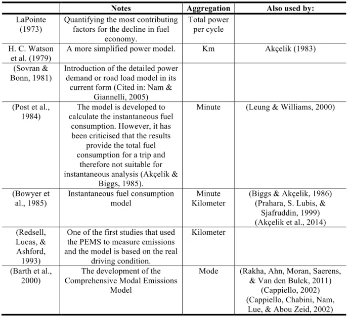
Table 2.4: A summary of the main literature modeling the power demand ... 57
Table 2.5: The summary of the emissions estimation packages ... 70
Table 3.1: The global descriptive statistics of the dataset ... 84
Table 4.1: The variation range of the variables ... 94
Table 4.2: Best selling cars in 2014 in Canada ... 97
Table 4.3: Honda Civic and Ford Escape fuel consumption ... 105
Table 4.4: The average impact of 10% variation of each variable on fuel consumption ... 105
Table 5.1: Definition of speed bins ... 114
Table 5.2: The relative humidity corresponding to temperatures in modified scenarios ... 117
Table 5.3: Comparing the sensitivity of speed and temperature ... 123
Table 6.1: Assessment criteria ... 130
Table 6.2: Cluster sequence using transition matrix and marcov modeling (CL stands for cluster) – example with 7 clusters ... 131
Table 6.3: Difference between the total average values of the assessment measures of the entire database and driving cycles for each method ... 136
Table A.1: The mean value CO2 emissions (g/s) for VSP modes for vehicles with engine displacement <3.5 L (Coelho et al., 2006)………..………..172
Table A.2: The correction coefficient f (T, V) to calculate the cold-start excess emissions for gasoline vehicle ………..………..………172 Table A.3: Coefficient a in the equation of the dimensionless excess emissions as a function of the dimensionless distance ………..………..………173 Table A.4: The cold distance calculation for CO2 emissions estimation………173 Table A.5: The impact of parking time on CO2 emissions………..173
LIST OF FIGURES
Figure 1.1: The global land-ocean temperature index (reproduced from: Hansen & Schmunk,
2011) ... 2
Figure 1.2: Total GHG emissions per province (Environment Canada, 2010) ... 5
Figure 1.3: GHG emissions by sector in 2004 (B. Metz et al., 2007) ... 7
Figure 1.4:Global anthropogenic GHG in 2004 (B. Metz et al., 2007) ... 7
Figure 1.5: GHG emissions by gas type in Quebec in 2012 (Delisle et al., 2015) ... 8
Figure 1.6: GHG emissions by sector in Quebec in 2012 (Delisle et al., 2015) ... 8
Figure 1.7: The structure of the thesis ... 29
Figure 2.1: General framework for carbon emissions estimation (reproduced from: Schipper, Cordeiro, & Ng, 2007) ... 31
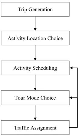
Figure 2.2: The four-step modeling framework ... 33
Figure 2.3: An example of the activity based model framework (Roorda & Miller, 2006) ... 35
Figure 2.4: An example of the emissions testing laboratory (MERILAB, 2008) ... 37
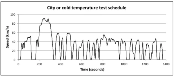
Figure 2.5: The city or the cold temperature test drive cycle (USEPA, 2015) ... 39
Figure 2.6: The highway test drive cycle (USEPA, 2015) ... 39
Figure 2.7: The air conditioning test drive schedule (USEPA, 2015) ... 39
Figure 2.8: The high speed/ quick acceleration test drive cycle (USEPA, 2015) ... 40
Figure 2.9: An example of PEMS by GlobalMRV company (GlobalMRV, 2015) ... 41
Figure 2.10: The vehicle power demand breakdown for the conventional SI engines ... 43
Figure 2.11: The excess CO2 emissions due to the AC ... 52
Figure 2.12: MOVES2014 Graphical User Interface ... 62
Figure 2.13: Data importer for county level ... 64
Figure 2.14: VERSIT+ model framework for Light Duty Vehicles (LDV) (Smit, Smokers, & Rabé, 2007) ... 67
Figure 2.15: Core structure of the IVE model (IVE model, 2008) ... 69
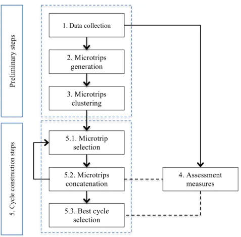
Figure 2.16. General process for developing driving cycles ... 72
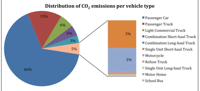
Figure 3.1: Distribution of total CO2 emissions per vehicle type (calculated by Quebec Ministry of Transportation using MOVES) ... 80
Figure 3.2: Data collection equipment and OBDII demonstration ... 81
Figure 3.3: The selected route for data collection ... 83
Figure 3.4: Speed-acceleration frequency distribution of the dataset ... 84
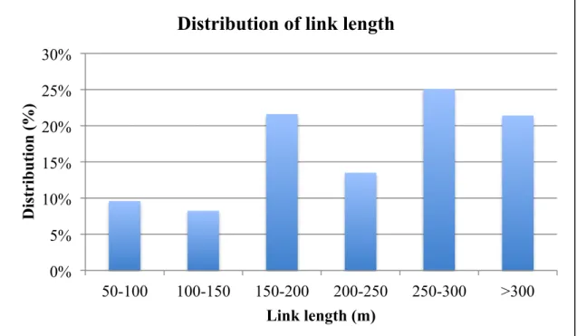
Figure 3.5: The road link length distribution ... 85
Figure 3.6: The link speed distribution ... 86
Figure 3.7: An example of the historical data provided by Government of Canada website ... 88
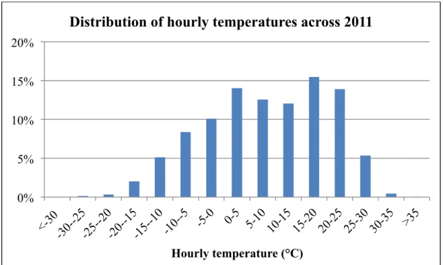
Figure 3.8: Hourly temperature distribution in Montreal throughout 2011 ... 89
Figure 4.1: The power demand distribution for the entire collected dataset ... 95
Figure 4.2: The impact of vehicle weight on power demand and fuel consumption ... 96
Figure 4.3: The impact of vehicle aerodynamics on power demand and fuel consumption ... 97
Figure 4.4: The impact of average speed on fuel consumption based on all the collected speed data ... 98
Figure 4.5: The impact of speed on power demand and fuel consumption ... 99
Figure 4.6: The impact of acceleration profile on fuel consumption ... 100
Figure 4.7: The impact of temperature on fuel consumption ... 101
Figure 4.8: The impact of wind speed on power demand and fuel consumption ... 102
Figure 4.9: The impact of road grade on power demand and fuel consumption ... 103
Figure 4.10: The fuel consumption tool developed in Excel environment ... 107
Figure 5.1: General schematic representation of Motrem-MOVES in inventory mode (Bourget, 2013) ... 111
Figure 5.2: Hourly temperature and humidity used in the baseline scenario based on the data
provided by MTQ as a part of Motrem MOVES dataset ... 112
Figure 5.3: Vehicle fleet in Montreal Island in 2011 based on the data provided by MTQ as a part of Motrem MOVES dataset ... 113
Figure 5.4: Total vehicle miles traveled based on the vehicle category on the Island of Montreal in 2011, the data is provided by MTQ as a part of Motrem MOVES dataset ... 113
Figure 5.5: CO2 emissions sensitivity to speed distribution for running and start exhaust emissions based on the data provided by MTQ as a part of Motrem MOVES dataset ... 116
Figure 5.6: Gasoline passenger vehicle age distributions for the baseline and modified scenarios based on the data provided by MTQ as a part of Motrem MOVES dataset ... 117
Figure 5.7: Correlation between CO2 emissions rate and average speedbin (for the definition of speedbins refer to Table 5.1) ... 119
Figure 5.8: CO2 emissions rate sensitivity to age distribution for running and start exhaust emissions ... 120
Figure 5.9 : CO2 emissions sensitivity to temperature for running and start exhaust emissions . 121 Figure 5.10: Total impact of temperature on CO2 emissions ... 121
Figure 5.11: CO2 emissions sensitivity to ramp fraction ... 122
Figure 6.1: Overall speed-acceleration time frequency distribution of the database ... 128
Figure 6.2: Average speed-acceleration time frequency distribution of microtrips related to congested urban driving pattern ... 128
Figure 6.3: Average speed-acceleration time frequency distribution of microtrips related to high speed, free-flow driving pattern ... 129
Figure 6.4: Distribution of microtrip duration for different methods used for identifying microtrips ... 133
Figure 6.5 Microtrip divisions based on MLE clustering algorithm on acceleration profile ... 134
Figure B.1: The average SAFD distribution of microtrips in cluster 1 ... 174
Figure B.3: The average SAFD distribution of microtrips in cluster 3 ... 175
Figure B.4: The average SAFD distribution of microtrips in cluster 4 ... 175
Figure B.5: The average SAFD distribution of microtrips in cluster 5 ... 176
Figure B.6: The average SAFD distribution of microtrips in cluster 6 ... 176
Figure B.7: The average SAFD distribution of microtrips in cluster 7 ... 177
Figure C.1: The driving cycle developed based on the stop sequence microtrip ... 178
Figure C.2: Driving cycle based on the 20-seconds microtrips ... 178
Figure C.3: The developed driving cycle based on 40-seconds microtrips ... 179
Figure C.4: The developed driving cycle based on 60-seconds microtrips ... 179
Figure C.5: The developed driving cycle based on 250-meter microtrips ... 180
Figure C.6: The developed driving cycle based on 500-meter microtrips ... 180
Figure C.7: The developed driving cycle based on 1000-meter microtrips ... 181
Figure C.8: The developed driving cycle based on intersection-based microtrips ... 181
Figure C.9: The developed driving cycle based on speed intervals microtrips ... 182
Figure C.10: The developed driving cycle based on microtrips defined by acceleration events by Maximum Likelihood Estimation (MLE) ... 182
Figure C.11: The developed driving cycle based on microtrips defined by acceleration events generated by k-mean method ... 183
Figure C.12: The developed driving cycle based on acceleration events defined by k-means method on average moving acceleration ... 183
LIST OF SYMBOLS AND ABBREVIATIONS
AC Air Conditioning
ARTEMIS Assessment and Reliability of Transport Emissions Models and Inventory Systems
CCAP Climate Change Action Plan CCF Congestion Correction Factor
CECERT College of Engineering Center for Environmental Research and Technology
CMEM Comprehensive Modal Emissions Model CNG Compressed Natural Gas
COPERT Computer Program to calculate Emissions from Road Transport
EC Engine Capacity
EMFAC Emissions Factors
EV Electric Vehicle
FC-VSL Fuel Consumption- Variable Speed Limit
GHG Greenhouse gases
GPS Global Positioning System GUI Graphical User Interface GWP Global Warming Potential
HBEFA Hand Book Emissions Factors for Road Transport
HDV Heavy-Duty Vehicle
HOV High Occupancy Vehicle
IPCC Intergovernmental Panel on Climate Change IRI International Roughness Index
ISA Intelligent Speed Adaptation IVE International Vehicle Emissions LCO Life Cycle Optimisation
LOS Level Of Service
MOVES Motor Vehicle Emissions Simulator MPD Mean Profile Depth
MTQ Ministry of Transportation Quebec OTAQ Office of Transportation and Air Quality PEMS Portable Emissions Measurement System
PHEM Passenger car and Heavy-duty Emissions Model RR Rolling Resistance
RRC Rolling Resistance Coefficient
SP Specific Power
TDM Travel Demand Management TEE Traffic Emissions and Energy U.S. United States
USEPA United States Environmental Protection Agency VKT Vehicle Kilometers Traveled
VSP Vehicle Specific Power
VTI The Swedish National Road and Transportation Research Institute WCI Western Climate Initiative
LIST OF APPENDICES
APPENDIX A - LOOK UP TABLES ... 172 APPENDIX B - THE SAFD DISTRIBUTION OF DIFFERENT CLUSTERS... 174 APPENDIX C - THE DRIVING CYCLE DEVELOPED BY DIFFERENT MICROTRIP METHODS THE SAFD DISTRIBUTION OF DIFFERENT CLUSTERS ...178
CHAPTER 1 INTRODUCTION
“Chart-topping June extends Earth’s warmest period on record”
(Samenow, 2015)
This somewhat incendiary headline echoes so many others in recent years, reporting the record-breaking weather conditions such as heat, cold, rainfalls, droughts, etc. When was the last time you heard about climate change or global warming? The subject has become a hotly debated question in scientific and political circles, with one question frequently arising: On whom, or where, can we place the blame?
1.1 Context
Climate change has become the top environmental concern over the past few decades. It is believed that the increase in the level of Greenhouse Gases (GHG) in the atmosphere is the main factor, and that the transportation sector can be traced back as the main contributor, specifically in North America (Atkins, 2009). In addition to climate change, the emissions coming from means of transportation can also affect air quality, noise level, water quality, soil quality, biodiversity, and land take (Rodrigue, Comtois, & Slack, 2013). Therefore, reduction in emissions from transportation has jumped to the beginning of the list of top priorities for almost every government. But what, exactly, is climate change? What are the consequences? How does transportation contribute to climate change? All these questions will be discussed in this introduction.
1.1.1 Climate change
As mentioned, climate change dilemma has become the first environmental challenge during the recent decades. We hear about climate change and its consequences almost every day. But how do we define climate and the anomalies of the climate?
Climate is basically referred to as the average weather conditions such as temperature, rainfall, wind direction and wind speed over the period of 30 years (B. Metz, 2010). Therefore, climate change is “a change in statistical properties of weather and climate at a place, in terms of average, variability, or both” (Arnell, 2015, p. 15). The primary indicator of climate change is the rise in the global temperature, that’s why it is often referred to as global warming. However, its consequences do not limit to the rise in the local temperature; contradictorily enough, the extreme cold can also be among the consequences. Figure 1.1 demonstrates the global land-ocean temperature variations since 1880. The records show a constant rise that has started more clearly around 1910s; the increase has been more dramatic since 1980s.
Figure 1.1: The global land-ocean temperature index (reproduced from: Hansen & Schmunk, 2011)
In addition to the temperature, climate change has a major influence on the environment; some of the main impacts are rise in the sea levels, multiplication of extreme weather events, the melting of glaciers, drought, and downpours. Some of these changes are irreversible such as the melting of glaciers and the extinction of species due to changes in
-0.6 -0.4 -0.2 0 0.2 0.4 0.6 0.8 1 1880 1900 1920 1940 1960 1980 2000 2020 Te m pe ra ture A nom al y ( oC) Year
Global Land-Ocean Temperature Index
their habitats (B. Metz, 2010). This fact emphasizes the immediate need to take action to avoid further damage. The first step towards defying climate change is identifying the main causes.
The causes of climate change can be classified in two categories: natural and anthropic. The main natural causes are solar radiation variations and volcanic eruptions. However, they are believed to be insignificant comparing to the anthropic causes. Scientists credit the raise in greenhouse gases (GHG) present in the atmosphere, produced by human activities, as the main guilty party for climate change (Crowley, 2000; B. Metz, 2010). Initially, the greenhouse gases do not have a negative impact on the earth; to the contrary, in normal levels, the concentration of greenhouse gases in the atmosphere regulates the temperature on earth. In fact, without them the earth would have been too cold for any living organisms to survive. Therefore, greenhouse gases are responsible for making the earth suitable for life due to the natural greenhouse effect they create. However, if the level of greenhouse gases rises, the temperature will rise as well; the earth is able to recover from just a certain amount of surcharge. But if the level increases faster than the natural trend (i.e. the enhanced greenhouse gas effect), the earth cannot cope with this surcharge and results in extreme conditions (Leroux, 2005).
The main greenhouse gases are water vapour (H2O), Carbon dioxide (CO2), Methane
(CH4), Nitrous oxide (N2O), Ozone (O3), Chlorofluorocarbons (CFCs), and carbon
tetrachloride (CCl4) (R. T. Watson, Meira Filho, Sanhueza, & Janetos, 1992). Among
those, Carbon dioxide is the most important anthropogenic greenhouse gas since it is produced significantly more than any other GHG (Intergovernmental Panel On Climate Change, 2007).
In the analysis of the impact of the greenhouse gases two measures are considered: the Global Warming Potential (GWP) and the lifetime in the atmosphere. GWP represents the cumulative radiative capacity of the gas to trap the heat in the atmosphere, relative to CO2, and the lifetime is the period that they can stay in the atmosphere before
changes over time and therefore its value is usually followed by the time it has been present in the atmosphere. Table 1.1 provides the 100-year GWP and the lifetime of some of the main regulated1 greenhouse gases. As we can see, some gases can stay in the atmosphere for hundreds of years.
Table 1.1: GWP and lifetime of the main greenhouse gases (IPCC, 2007)
Name of gas Chemical formula Atmospheric lifetime (years) 100-year GWP
Carbon dioxide CO2 50-200 1 Methane CH4 9-15 21 Nitrous oxide N2O 114 310 Hydrofluorocarbons HFCs 1.4 - 270 140 – 11,700 Chlorofluorocarbons CFCs 45 – 1,700 3,800 – 8,100 Carbon tetrachloride CCl4 26 1,400
The recent analysis of the Intergovernmental Panel on Climate Change (IPCC) in the 4th assessment report indicates that a 50% to 80% reduction of global GHG emissions by 2050, from the year 2000’s levels, is required to avoid serious consequences (Ohnishi, 2008). Since the 1990s, different national and international frameworks have been proposed to reduce greenhouse gases; in the following section a brief review of those will be provided.
1.1.2 Policies regarding the GHG emissions reduction
The Kyoto Protocol is the only international and legally binding agreement to tackle climate change so far. It commits its parties to achieve an international goal for the reduction of greenhouse gas emissions (United Nations, 2015). The protocol was adopted in Kyoto, Japan in 1997 and entered in force in 2005. The first commitment period started in 2008 and ended in 2012. Based on the Kyoto Protocol, the countries contributing to an overall 55% of the GHG emissions, approved to respect a certain target. However, among
them the United Stated2 and Australia did not accept to commit (Sperling & Cannon, 2007).
After the first round, the new commitment, referred to as the “Doha Amendment to Kyoto Protocol”, was adopted in 2012. Based on this amendment, 37 industrialized countries agreed to reduce their GHG emissions 18% below the 1990 level in an eight-year period from 2013 to 2020 (United Nations, 2015). Initially Canada was among the countries that committed to the protocol but withdrew in 2011 (Curry & McCarthy, 2011).
However, despite the withdrawal of Canada, Quebec was the first province to take action toward GHG emissions reduction and to push ahead with its climate change action plan (Teisceira-Lessard, 2011). Comparing to the other Canadian provinces, Quebec is among the least emitters (Figure 1.2).
Figure 1.2: Total GHG emissions per province (Environment Canada, 2010)
2 U.S. is second largest CO
2 emitter after China and responsible for about 16% of the global CO2 emissions. 0 50 100 150 200 250 300 NL PE NS NB QC ON MB SK AB BC YT NT M ega tonne s of CO 2 e qui va le nt
GHG emissions in Canada by provinces
Based on the province of Quebec’s action plan, the objective is to reduce the GHG emissions to 20% below the 1990 level by the year 2020. Quebec’s commitment to achieving its goal follows the 2012 Climate Change Action Plan (CCAP 2006-2012) adopted in the Kyoto Protocol framework. As a part of this action plan, Quebec has established a carbon market ("Québec in action!," 2012), a program coordinated with the Western Climate Initiative (WCI), a North American organization focused on tackling climate change. Through the first phase, starting on the 1st of January 2013, large industrial emitters are obliged to comply with the program. In its second phase, starting from January 2015, enterprises that distribute or import fossil fuels in Quebec will also have to comply with the system ("Québec in action!," 2012). In a carbon market or cap-and-trade system, basically, each enterprise has a certain allowance to produce GHG emissions. If they produce more, they have to buy more allowance from the carbon market to cover their surcharge and if they produce less they can sell the extra allowance. It is at this point that we became familiar with some of the main emissions reduction programs on an international level, as well as national and provincial. The next step to decrease the GHG emissions is to identify the main contributors.
1.1.3 Who is responsible for the GHG emissions
From a global perspective, the energy supply contributes the most to the GHG emissions, being responsible for about 26%. After that, industry, forestry, and agriculture are the biggest emitters, followed by transport, buildings and waste (B. Metz, Davidson, Bosch, Dave, & Meyer, 2007). Also, among all the greenhouse gases, the share of CO2 is the
However, the share of each sector is different in different regions. Specifically, the source of electricity has a very significant influence on the contribution of each sector. For example, in Quebec, about 45% of greenhouse gases emissions is produced by transport, and among different gases, CO2 amounts to 80% of it (Delisle, Leblond, Nolet, & Paradis,
2015).
The main focus of this study is the province of Quebec; and knowing that the transportation sector is the main contributor in Quebec and CO2 having the highest share
among the different greenhouse gases, this study is focused on the CO2 emissions from
the transportation sector. In the following section, policies and strategies regarding emissions reduction in transportation sector will be reviewed.
Figure 1.3: GHG emissions by sector in 2004 (B. Metz et al., 2007)
Figure 1.4:Global anthropogenic GHG in 2004 (B. Metz et al., 2007) Energy supply 26% Industry 19% Forestry 17% Agriculture 14% Transport 13% Residential and commercia l buildings 8% Waste and wastewate r 3%
Global GHG emissions by sector in 2004 N2O 8% F-‐gases 1% CO2 fossil use 57% CO2 other 3% CO2 (deforestat ion, decay of biomass, etc) 17% CH4 14% Global anthropogenic GHG emissions in 2004
Figure 1.5: GHG emissions by gas type in Quebec in 2012 (Delisle et al., 2015)
Figure 1.6: GHG emissions by sector in Quebec in 2012 (Delisle et al., 2015) 1.1.4 CO2 emissions reduction strategies in transportation sector
Before discussing further, it is important to mention that CO2 emissions are proportional
to the fuel consumption; each litre of gasoline produces 2.4 kg of CO2 on average.
Therefore, the fuel consumption and CO2 emissions is often used interchangeably in this
study. The following equation demonstrates the general chemical equation of complete gasoline combustion.
𝑛!𝐶!𝐻!+ 𝑚!𝑂! → 𝑛!𝐻!𝑂 + 𝑚!𝐶𝑂! Equation 1-1
In general, the amount and variability of emissions from transportation is influenced by four main elements: travel demand, mode share, fuel type, and fuel economy (Ohnishi, 2008). Keeping that in mind, reduction in emissions can be achieved by making modifications to these elements. Therefore, an integrated transport policy for emissions reduction would consist of the following methods (B. Metz, 2010):
1. Reduce demand: lower need for transport N2O 6% PFC 1% HFC 2% SF6 0% CO2 80% CH4 11%
GHG emissions by gases in Quebec 2012 Transport 45% Energy 0% Waste 5% Agricultur e 8% Residenti al and commerci al building 10% Industry 32%
GHG emissions by sector in Quebec 2012
2. Shift means of transport: shifting to less emitting modes such as active transportation
3. Change the fuel: shift from oil products to less polluting and less carbon intensive fuels
4. Improve efficiency: reduce the fuel consumption of vehicles
Each of these elements is broken down to the more tangible policies in the following sections.
1.1.4.1 Travel demand and mode shift
Private vehicle ownership has been increasing around the world and, consequently, the energy consumption and emissions are continuing to increase (Poudenx, 2008). Undoubtedly the best way to decrease emissions would be decreasing the trips or changing the mode towards more efficient modes. Since most of the strategies for emissions reduction touch upon both travel demand and travel mode, we discuss both, together, in this section.
The first and most important measure to reduce vehicle emissions is to reduce vehicle activity; fewer Vehicle Kilometers Traveled (VKT) results in less emissions. In the early 1970s in the United States, due to the booming travel demand, the transportation policy makers started to think of how to satisfy the increasing demand without increasing the capacity and building more roads (Meyer, 1999). Travel Demand Management (TDM) programs came into being with an aim to use the most out of the available network. Some of the proposed TDM policies are (Gärling et al., 2002):
1. Taxation of cars and fuels
2. Closure of city centers for car traffic 3. Road pricing
4. Parking control
6. Avoiding major new road infrastructure 7. Teleworking
8. Land use planning that encourages shorter travel distances
9. Traffic management reallocating space between modes and vehicles (e.g. bus and high occupancy vehicle lanes)
10. Park and ride schemes
11. Improved public transport (e.g. frequency, comfort, retrievability of information about public bus and high occupancy vehicles lanes)
12. Improved infrastructure for walking and biking
13. Public information campaigns about the negative effects of driving
14. Social modeling where prominent public figures use alternative travel modes
The impact of these strategies largely depends on the travel behaviour and the specific characteristics of each region. For example, in a study of comparison of the TDM strategies in the U.S. (Meyer, 1999), it is discussed that the congestion pricing has the highest impact on the number of trips, whereas the bike/pedestrian infrastructure has a very low impact.
Also Gärling and Schuitema (2007) believe that coercive measures such as pricing have more impact on trip reduction; however, when it is paired up with the non-coercive measures, it is the most effective. The road pricing in London is considered one of the successful examples, which could reduce CO2 levels by 20% by reducing the vehicle trips
(Beevers & Carslaw, 2005)3. In addition to the reduction in the total private vehicle trip, increasing the fees can encourage a mode shift. The mode shift toward the active transportation can have a significant impact on reducing the vehicle use.
3 They examined the impact of the pricing on emissions through changes in speed profile, but they found it
Godefroy and Morency (2012) estimated the potential of about 18% reduction in private vehicle trips, in Montreal (Quebec), by replacing them with bike and walk. In their study they considered the geographical, demographic, and travel behaviour to calculate the feasibility of biking or walking. However, sometimes the personal preference makes a big difference; many prefer to drive despite the fact that walking or biking is a viable alternative.
Another strategy that can have an important influence on emissions, specifically through a reduction in the number of trips, is telecommuting. A comparison of participants' telecommuting day travel behaviour with their before-telecommuting behaviour in Australia shows a 27% reduction in the number of personal vehicle trips, a 77% decrease in VKT, and 39% (and 4%) decreases in the number of cold (and hot) engine starts (Koenig, Hensher, & Puckett, 2007). All these changes can have a significant reduction on emissions. Overall, the strategies that result in the lower VKT or mode shift are considered the most effective regarding the GHG emissions.
1.1.4.2 Fuel type
Along with the change in travel demand and mode, fuel is one of the main determinants of the vehicle emissions levels. The research on more efficient and less pollutant fuels is numerous, and as a result various alternative fuels have been introduced and evaluated. In general, fuels can be classified in two categories: conventional fuels and alternative fuels. In road transportation, conventional fuels refer to gasoline and diesel. Historically, in comparing these two fuels regarding their contribution to CO2 emissions, it has been
believed that the diesel engine produces less CO2 for the same power output. Yet, due to
recent improvements to the gasoline engine efficiency this gap has been reduced (Sullivan et al., 2004). Nevertheless, diesel and gasoline are both fossil fuels, and come with a high carbon concentration. Considering the urgent need to reduce the carbon emissions, more and more studies are focused on the types of fuels with a lesser carbon content.
Some of those main alternative fuels are: biodiesel, bioethanol, hydrogen cell, solar energy, compressed natural gas, and electricity. Each of these alternative fuels has its
advantages and disadvantages. To evaluate the alternative fuels, from the provider’s perspective, the following factors are commonly considered (Jahirul et al., 2010):
15. acceptability of fuel supply, 16. process efficiency,
17. ease of transport and safety of storage, 18. vehicle modifications needed, and
19. fuel compatibility with vehicle engine (power, emissions, ease of use, and durability of engine)
In addition, from the users’ perspective, some of the challenges of the alternative fuels consist of (Romm, 2006):
- the higher cost of the vehicle, - on-board fuel storage,
- safety and liability, - high fuelling cost, and - limited fuel stations.
For example, solar powered engines are not market adaptive yet and require further research on the design of the engine (Jahirul et al., 2010). Also, regarding the hydrogen engines, the volumetric efficiency is much less than that of gasoline-powered engines (White, Steeper, & Lutz, 2006). Besides there are important safety concerns over the transportation and storage of the fuel (Chalk & Miller, 2006).
Meanwhile, there are some other alternative fuels that are easier to adopt such as biodiesel and bioethanol that require minor to no engine modification. Bioethanol, specifically, could provide a fuel with no carbon dioxide emissions (Lave, MacLean, Hendrickson, & Lankey, 2000). In addition, mixing ethanol with gasoline can also provide carbon reduction benefits. For example 85% of ethanol (E85) can reduce emissions by 70%
(USEPA, 2006). However, taking the engine performance in to account, a 20% blend offers the best performance and still reduces CO2 emissions by 7.5% (Al-Hasan, 2003).
Biodiesel, on the other hand, does not reduce the CO2 emissions but also increases the
fuel consumption and CO2 emissions due to deteriorated engine efficiency. In the case of
biodiesel the impact largely depends on the driving behaviour and the engine load; the least efficient events were observed under low speed, in low load condition (Fontaras et al., 2009). However, regarding the lifetime assessment, both bioethanol and biodiesel have brought up certain concerns regarding the environmental impact and the threat to food security (Escobar et al., 2009).
Furthermore, it is discussed that Compressed Natural Gas (CNG) can represent a good alternative fuel for Spark Ignition (SI) engines and can be the future fuel for transportation and has become very popular in some countries. The CNG can reduce the CO2 by up to 20% and requires minor modifications to the conventional spark ignition
engine (Gopal & Rajendra, 2012).
In addition, the introduction of the Electric Vehicles (EV) as Zero Emissions Vehicles (ZEV) seems to be the ultimate solution for emissions reduction. However, the source and the processing of energy production and storage, as well as the lifetime of the vehicle, play an important role in defining the benefit of these types of vehicle. The EV vehicles can only be environmentally beneficial if the electricity is produced from low carbon sources (C. Samaras & Meisterling, 2008). Otherwise, it is claimed that the electricity being produced by high carbon sources can even increase the life cycle carbon emissions since the electric engines are not very energy efficient (Helms, Pehnt, Lambrecht, & Liebich, 2010).
The cost and benefit analysis of the electric vehicles is a sensitive subject. The methodology of the life cycle assessment of the electric vehicles can play a significant role in determining its benefits. In one study, it is discussed that just by overestimating the lifetime of the EVs, the benefit has been overestimated by about 28%; whereas, the environmental benefit can be reduced by up to 14% in case of more realistic lifetime
assumptions (Hawkins, Singh, Majeau-Bettez, & Strømman, 2012). However, it is important to note that all estimations can change significantly in different regions due to the difference in the source of electricity production and geographical and climatic characteristics. Also, due to the rapid advancement of the EV technology, the assessments require regular updates.
It should also be noted that although the new technologies in vehicle and fuel can decrease the fuel consumption, any transformation in the fleet would be gradual. Every year only 7% of the in-use vehicles are replaced by new vehicles (Barkenbus, 2010) and among those a small percentage is dedicated to low carbon emissions vehicles. The process of moving toward alternative fuels could take decades; therefore, it is important to keep working on improving the conventional fuel vehicles in parallel to introducing and implementing new vehicle technologies.
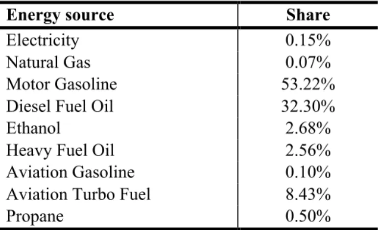
In Canada more than 80% of the energy used in transportation (passenger, freight and off road) is based on gasoline and diesel, which confirms the importance of these fuels in emissions reduction strategies. Table 1.2 shows the share of each fuel type in the total energy production across Canada, which includes passenger, freight and off-road (Statistics Canada, 2014).
Table 1.2: Share of different fuel types in energy production in transportation in Canada 2012
Energy source Share
Electricity 0.15%
Natural Gas 0.07%
Motor Gasoline 53.22%
Diesel Fuel Oil 32.30%
Ethanol 2.68%
Heavy Fuel Oil 2.56%
Aviation Gasoline 0.10%
Aviation Turbo Fuel 8.43%
Propane 0.50%
Regarding motor gasoline, there are some improvements that can be made to reduce the CO2 emissions such as modifying the levels of sulphur inherent to the gasoline and of the
(<10 ppm) fuels by the European Comission (2001), it is discussed that the modification can reduce the total CO2 emissions by 347.1 kt, even considering the additional emissions
produced by the refineries themselves; another 3% improvement in fuel economy is also observed through the use of detergent additives to the fuel (Karpov, 2007). However, Canada falls behind in this matter and has set the required gasoline sulphur level to a yearly pool average of 30 ppm, with a maximum of 80 ppm, which is much higher than the European legislation (Row & Doukas, 2008). Therefore the quality of the fuel is one of the factors that still can be enhanced, especially in certain locations.
As mentioned above, gasoline is the most popular fuel used in North America and the shift towards alternative fuel is gradual and might even take decades. Therefore, this study is focused on the regular SI gasoline vehicle. However, it is necessary to keep in mind other possibilities, although analyzing all the fuel types or transportation modes would not fit into this study. So far, the travel demand, travel mode and fuel type have all been discussed briefly. In the following section, the subject of vehicle economy and the policies regarding emissions reduction through the improvement of fuel economy of the gasoline passenger vehicles will be discussed in more detail.
1.1.4.3 Vehicle fuel economy
The shift towards greener fuel or a reduction in travel demand can be a slow process, mainly due to the high costs of infrastructure (especially in the case of fuel) and acceptability of the projects (both regarding the modification of the travel behaviour or mode and the fuel shift). Meanwhile, other policies and strategies should be taken into consideration. The strategies can be classified in two categories; the first category focuses on improving the fleet by improving the new vehicles’ technologies and removing the old cars from the fleet. The second category of strategies mainly has a direct or an indirect impact on vehicle utilisation and driver behaviour. In this section, both categories and the main relevant strategies will be looked at.
In the first category, the strategies regarding the vehicle’s characteristics consist of the policies that can affect vehicular emissions by regulating or modifying the vehicle, and
are independent of the vehicle utilisation factor or driver behaviour. The most significant of those are the regulations and standards set by the governments aimed at the vehicle manufacturers. These regulations are focused on improving the vehicle economy through the improvement of vehicular technology. Also, encouraging the scrapping of old cars currently still in-use is a complimentary regulation to improve the fuel efficiency of the entire fleet in a shorter period. Policy makers are mainly pushing for more efficient vehicles, alternative fuels and reducing kilometers traveled. However, as mentioned earlier, modifying the fleet can be a slow process. Meanwhile, there are other strategies that can help reduce the vehicle CO2 emissions with the current fleet characteristics.
The second category of strategies, mainly influencing the driving pattern, can be approached with two different perspectives: traffic management and eco driving. While traffic management strategies are the ones conducted by the authorities, eco-driving is among the strategies adopted by the drivers themselves. All, these strategies will be introduced in this section.
Regulations for manufacturers
First and foremost, in a larger scale, the national governments are responsible to oblige the vehicle manufacturers to produce more fuel-efficient vehicles. The vehicles’ pollution emissions standards have been around for a while but it is only recently that the GHG emissions became regulated. In Canada, the first Passenger Automobile and Light Truck
Greenhouse Gas Emissions Regulations was established in 2010 to reduce the greenhouse
gas emissions by setting emissions standards and test procedures that were aligned with the regulations in the U.S. This new regulation required the automobile makers to reduce the GHG emissions of their fleet starting in 2011 through 2016.
The more recent amendment to this regulation regards the vehicles from 2017 and beyond, and aims to reduce the GHG emissions of the fleet by 50% in 2025, comparing to the level from 2008. Based on that, over the lifetime operation of 2017 to 2025 model year vehicles, the regulation is projected to deliver the total GHG reductions of 174 megatons, roughly equivalent to one year of GHG emissions from Canada’s entire
transportation sector (Environment Canada, 2014). However, without eliminating the old high-consumption vehicles, the improvement of the fuel efficiency of the entire fleet can be slower; therefore it is necessary to implement a complimentary regulation for scrapping the old vehicles at the same time.
Scrapping old cars
It is expected that, not considering other factors, the shorter the average lifetime of the vehicle is, the lower the energy consumption and emissions would be; this is all considering the older vehicles produce higher emissions because of the degradation of their emissions control systems4 (Lawson, 1993; Ntziachristos & Samaras, 2000; Z. Samaras et al., 1998; Zachariadis, Ntziachristos, & Samaras, 2001). Programs intended for scrapping old cars have been introduced in the 1990s in many countries to reduce vehicle emissions from the more emissions-prone older vehicles. However, all is not as simple as that. It is true that the older vehicles have higher emissions rates, but at the same time, the process of making new vehicles or scrapping the old vehicles also produces high emissions.
With this in mind, it is crucial to assess the life cycle emissions rather than just the tailpipe emissions. If the vehicles are scrapped earlier than their efficient lifetime, the whole process can produce even more emissions unless the trend of fuel economy improvement changes much faster than the historical data would indicate (Van Wee, Moll, & Dirks, 2000). In the same study, the authors mentioned that in an evaluation of the life-cycle energy requirements of new cars in the Netherlands between 1990 and 1994, 15 to 20% of the life-cycle energy requirement is linked to car production, maintenance and disposal; the remaining 80 to 85% is related to the fuel consumption for car driving. Therefore, it is very important to determine the most efficient lifespan of the vehicles. The
4 However, no significant relation between the mileage and CO
2 emissions has been found (P. Boulter, 2009; P.
analysis highlights that the newer vehicles on the road do not necessarily result in less global emissions.
There are several life cycle assessment tools and approaches to analyze the lifespan of the vehicles. In one study of calculating the optimised life cycle of the vehicle, it is discussed that the optimal life of the vehicle regarding the cumulative CO2 emissions is 18 years,
based on driving 12,000 km/year (Kim, Keoleian, Grande, & Bean, 2003). In their study, they applied the Life Cycle Optimization (LCO) model to mid-sized passenger car models between 1985 and 2020. It is important to note that these numbers cannot be generalised; each region can have its own optimal vehicle lifespan depending on the local fleet and even the environmental characteristics.
In addition to the composition of the fleet, the Vehicle Kilometers Traveled (VKT) can play an important role in the total fleet emissions. For example, it is believed that older vehicles are driven less (Van Wee et al., 2000); therefore, they can have a less important share in the global emissions.
Traffic management
In regards to emissions reduction, traffic management strategies can consist of three main perspectives: congestion mitigation, speed management, and traffic smoothing. Most of the strategies touch on all three perspectives at the same time and can hardly be discussed separately. Traffic congestion is a very hot topic in traffic engineering and transportation planning. However, it is largely overlooked as a solution for reducing CO2 emissions. As
a simplistic approach, when congestion increases, vehicles drive for longer time and therefore the fuel consumption and CO2 emissions increase accordingly. In addition,
traffic management strategies not only have influence on travel time, but also impact the driving behaviour elements such as speed and the frequency of acceleration/deceleration. There are various strategies to decrease the traffic congestion and improve the traffic fluidity. Various studies have claimed that traffic signal timing and coordination is among the most common traffic management strategies that can improve fuel consumption or reduce CO2 emissions significantly (Unal, Rouphail, & Frey, 2003). For example, in one
study using a traffic simulation model (VISSIM) for a signal coordination on a highway, the authors reported a 9% of CO2 emissions reduction (Zhang et al., 2009). Also in
another study, again using a microsimulation model, it was observed that the coordinated traffic light that creates green waves along major arterials is not only beneficial for CO2
emissions reduction, but also in lowering air and noise pollution by reducing the acceleration and deceleration of vehicles (De Coensel, Can, Degraeuwe, De Vlieger, & Botteldooren, 2012).
The traffic management strategies are usually focused on increasing the vehicles’ speed; however, it is important to note that a higher speed does not necessarily mean lower emissions. On the contrary, if the vehicles drive too fast on the highway, that can increase fuel consumption due to the increased aerodynamic resistance of the vehicles. The speed and fuel consumption per kilometer has a U-shaped relation, meaning that the fuel consumption decreases by the increase of the speed to an optimal level (about 80 km/h) and it starts to increase after. The optimal speed however can be different depending on the technology of the vehicle engine and its aerodynamics. Also, higher speed can mean more frequent and brusquer acceleration and deceleration. In order to avoid that, Intelligent Speed Adaptation (ISA) has been introduced.
ISA is basically an in-vehicle electronic system that enables the speed regulation; it is connected to a GPS and map, and whenever the speed exceeds the posted speed the fuel is cut off. However, in an analysis of the ISA method, Int Panis, Broekx, and Liu (2006) discussed that the benefit of the ISA is dependent on the situation and they did not find any statistically significant impact on the CO2 emissions. In another study, a similar but
more intricate scheme has been analyzed. In that study, Bojin, Ghosal, Chen-Nee, and Zhang (2012) introduced a carbon foot print/ fuel consumption-aware variable speed limit (FC-VSL) that regulates the speed based on various measures, such as road conditions, and communicates in real time with the road-side infrastructures that are connected to a control center, which evaluates the road conditions and determines the optimal speed. Their results of the study showed that in contrast to ISA, this method could bring
significant improvement on fuel consumption or CO2 emissions due to the traffic
smoothing effect that it offers.
Another traffic management strategy for smoothing the traffic flow is through the replacement of signalized intersections with roundabouts. It is claimed that this strategy can reduce fuel consumption by 28% and 3% for replacing signalised yield-regulated junctions (Várhelyi, 2002). In this study, the author studied 20 yield-regulated intersections and 1 signalised intersection that were converted to roundabouts to improve the safety. Also, in another study with more samples, in Kansas and Nevada, Mandavilli, Rys, and Russell (2008) confirmed the results of the previous study and presented even higher benefits (16-59%) both for AM and PM peak periods. However, Ahn, Kronprasert, and Rakha (2009) in another effort explained that the environmental benefit of the roundabout depends on the road type and demand. They explained that at the intersection of a high speed and a low speed road, the roundabout does not necessarily reduce fuel consumption. In their case study, the roundabout reduced the delay and the queue length at the intersection but the high acceleration following the roundabout increased fuel consumption considerably. As a result, the roundabouts are most efficient when approaching traffic volumes are relatively low. However, even in low speed traffic, when demand increases it can result in a substantial increase in delay comparing to the signalised intersections.
In addition to the intersection design, in the same category of road design, there’s also some evidence that the lane’s layout might have an influence on fuel consumption. For example in a study of High Occupancy Vehicle (HOV) lanes in California, it is revealed that a constant access to a HOV lane produces less CO2 emissions and that’s mainly due
to the highly concentrated manoeuvring on the dedicated ingress/egress sections, which causes higher frequency and magnitude of acceleration and deceleration (Boriboonsomsin & Barth, 2008).
It is important to mention that the environmental assessment of the traffic management strategies is very complex and requires detailed analysis of the driving behaviour and