HAL Id: hal-01701688
https://hal.archives-ouvertes.fr/hal-01701688
Submitted on 6 Feb 2018
HAL is a multi-disciplinary open access
archive for the deposit and dissemination of
sci-entific research documents, whether they are
pub-lished or not. The documents may come from
teaching and research institutions in France or
abroad, or from public or private research centers.
L’archive ouverte pluridisciplinaire HAL, est
destinée au dépôt et à la diffusion de documents
scientifiques de niveau recherche, publiés ou non,
émanant des établissements d’enseignement et de
recherche français ou étrangers, des laboratoires
publics ou privés.
Learning for Energy Harvesting Wireless Sensor
Networks
Fayçal Ait Aoudia, Matthieu Gautier, Olivier Berder
To cite this version:
Fayçal Ait Aoudia, Matthieu Gautier, Olivier Berder. RLMan: an Energy Manager Based on
Rein-forcement Learning for Energy Harvesting Wireless Sensor Networks. IEEE Transactions on Green
Communications and Networking, IEEE, 2018, pp.1 - 11.
�10.1109/TGCN.2018.2801725�.
�hal-01701688�
RLMan: an Energy Manager Based on
Reinforcement Learning for Energy Harvesting
Wireless Sensor Networks
Fayçal Ait Aoudia, Matthieu Gautier, Olivier Berder Univ Rennes, CNRS, IRISA
Email: {faycal.ait-aoudia, matthieu.gautier, olivier.berder}@irisa.fr
Abstract—A promising solution to achieve autonomous wireless sensor networks is to enable each node to harvest energy in its environment. To address the time-varying behavior of energy sources, each node embeds an energy manager responsible for dynamically adapting the power consumption of the node in order to maximize the quality of service while avoiding power failures. A novel energy management algorithm based on reinforcement learning, named RLMan, is proposed in this work. By contin-uously exploring the environment, RLMan adapts its energy management policy to time-varying environment, regarding both the harvested energy and the energy consumption of the node. Linear function approximations are used to achieve very low computational and memory footprint, making RLMan suitable for resource-constrained systems such as wireless sensor nodes. Moreover, RLMan only requires the state of charge of the energy storage device to operate, which makes it practical to implement. Exhaustive simulations using real measurements of indoor light and outdoor wind show that RLMan outperforms current state of the art approaches, by enabling almost 70 % gain regarding the average packet rate. Moreover, RLMan is more robust to variability of the node energy consumption.
I. INTRODUCTION
Many applications, such as smart cities, precision agriculture and plant monitoring, rely on the deployment of a large num-ber of individual sensors forming Wireless Sensor Networks (WSNs). These individual nodes must be able to operate for long periods of time, up to several years or decades, while being highly autonomous to reduce maintenance costs. As refilling the batteries of each device can be expensive or impossible if the network is dense or if the nodes are deployed in a harsh environment, maximizing the lifetime of typical sensors powered by individual batteries of limited capacity is a perennial issue. Therefore, important efforts were devoted in the last decades to develop low power consumption devices as well as energy efficient algorithms and communication schemes to maximize the lifetime of WSNs. Typically, a node quality of service (sensing rate, packet rate. . . ) is set at deployment to a value that guarantees the required lifetime. However, as batteries can only store a finite amount of energy, the network is doomed to die.
A promising solution to increase the lifetime of WSNs is to enable each node to harvest energy in its environment. In
This work was already partially published in the proceedings of the IEEE International Conference on Communications 2017 (IEEE ICC17).
this scenario, each node is equipped with one or more energy harvesters, as well as an energy buffer (battery or capacitor) to allow storing part of the harvested energy for future use during periods of energy scarcity. Various energy sources are possible [1], such as light, wind, motion, fuel cells. . . . As the energy sources are typically dynamic and uncontrolled, it is required to dynamically adapt the power consumption of the nodes, by adjusting their quality of service, in order to avoid power failure while maximizing the energy efficiency and ensuring the fulfilment of application requirements. This task is done by a software module called Energy Manager (EM). For each node, the EM is responsible for maintaining the node in Energy Neutral Operation (ENO) [2] state, i.e., the amount of consumed energy never exceeds the amount of harvested energy over a long period of time. Ideally, the amount of harvested energy equals the amount of consumed energy over a long period of time, which means that no energy is wasted by saturation of the energy storage device.
Many energy management schemes were proposed in the last years to address the non trivial challenge of designing ef-ficient adaptation algorithms, suitable for the limited resources provided by sensor nodes in terms of memory, computation power, and energy storage. They can be classified based on their requirement of predicted information about the amount of energy that can be harvested in the future, i.e., prediction-based and prediction-free. Prediction-based EMs [2]–[5] rely on pre-dictions of the future amount of harvested energy over a finite time horizon to take decision on the node energy consumption. In contrast with prediction-based energy management schemes, prediction-free approaches do not rely on forecasts of the harvested energy. These approaches were motivated by (i) the significant errors from which energy predictors can suffer, which incur overuse or underuse of the harvested energy, and (ii) the fact that energy prediction requires the ability to measure the harvested energy, which incur a significant overhead [6]. Indeed, most of the EMs require an accurate control of the spent energy, as well as detailed tracking of the previously harvested and previously consumed energies to operate properly.
Considering these practical issues, we propose in this paper RLMan, a novel EM scheme based on Reinforcement Learning (RL) theory. RLMan is a prediction-free EM, whose objective is to maximize the quality of service, defined as the packet rate, i.e., the frequency at which packets are generated (e.g., by performing measurements) and sent, while avoiding power
failure. It is assumed that the node is in the sleep state between two consecutive packet generations and sendings, in order to allow energy saving. RLMan requires only the state of charge of the energy storage device to operate and aims to set the packet rate by both exploiting the current knowledge of the environment and exploring it, in order to improve the policy. Continuous exploration of the environment enables adaptation to varying energy harvesting and energy consumed dynamics, making this approach suitable for the uncertain environment of Energy Harvesting WSNs (EH-WSNs). The problem of maximizing the quality of service in EH-WSNs is formulated as a Markovian Decision Process (MDP), and a novel EM scheme based on RL theory is introduced. The major contributions of this paper are:
‚ A formulation of the problem of maximizing the quality
of service in energy harvesting WSNs using the RL framework.
‚ A novel EM scheme based on RL theory named RLMan,
which requires only the state of charge of the energy storage device, and which uses function approximations to minimize the memory footprint and computational overhead.
‚ An exploration of the impact of the parameters of
RL-Man using extensive simulations, and real measurements of both indoor light and outdoor wind.
‚ The comparison of RLMan to three state-of-the-art EMs
(P-FREEN, Fuzzyman and LQ-Tracker) that aim to max-imize the quality of service, regarding the capacitance of the energy storage device and the variability of the node task energy cost.
The rest of this paper is organized as follows: Section II presents the related work focusing on prediction-free EMs, and Section III provides the relevant background on RL theory. In Section IV, the problem of maximizing the packet rate in energy harvesting WSNs is formulated using the RL framework, and RLMan is derived based on this formulation. In Section V, RLMan is evaluated. First, the simulation setup is presented. Next, exploration of the parameters of RLMan is performed. Finally, the results of the comparisons of RLMan to three other EMs are shown. Section VI concludes this paper.
II. RELATED WORK
The first prediction-free EM was LQ-Tracker [7], proposed in 2007 by Vigorito et al.. This scheme relies on linear quadratic tracking, a technique from control theory, to adapt the duty-cycle according to the current state of charge of the energy buffer. In this approach, the energy management prob-lem is modeled as a first order discrete time linear dynamical system with colored noise, in which the system state is the state of charge of the energy buffer, the controller output is the duty-cycle and the colored noise is the moving average of state of charge increments produced by the harvested energy. The objective is to minimize the average squared tracking error between the current state of charge and a target residual energy level. The authors used classical control theory results to get the optimal control, which does not depend on the colored noise, and the control law coefficients are learned online using
gradient descent. Finally, the outputs of the control system are smoothed by an exponential weighting scheme to reduce the duty-cycle variance.
Peng et al. proposed P-FREEN [8], an EM that maximizes
the duty-cycle of a sensor node in the presence of battery storage inefficiencies. The authors formulated the average duty-cycle maximization problem as a non-linear programming problem. As solving this kind of problem directly is computa-tionally intense, they proposed a set of budget assigning prin-ciples that maximizes the duty-cycle by only using the current observed energy harvesting rate and the residual energy. The proposed algorithm requires the current state of charge of the energy buffer as well as the harvested energy to take decision about the energy budget. If the state of charge of the energy buffer is below a fixed threshold or if the amount of energy harvested at the previous time slot is below the minimum required energy budget, then the node is operating with the minimum energy budget. Otherwise, the energy budget is set to a value that is a function of both the amount of energy harvested at the previous time slot and the energy storage efficiency.
In [9] the authors proposed to use fuzzy control theory to dynamically adjust the energy consumption of the nodes. Fuzzy control theory proposes to extend conventional con-trol techniques to ill-modeled systems, such as EH-WSNs. With this approach, named Fuzzyman, an intuitive strategy is formally expressed as a set of fuzzy IF-THEN rules. The algorithm requires as an input both the residual energy and the amount of harvested energy since the previous execution of the EM. The first step of Fuzzyman is to convert the crisp entries into fuzzy entries. The so-obtained fuzzy entries are then used by an inference engine which applies the rule base to generate fuzzy outputs. The outputs are finally mapped to a single crisp energy budget that can be used by the node. The main drawbacks of Fuzzyman are that it requires the amount of energy harvested which can be unpractical to measure, and the lack of systematic way to set the parameters.
RL theory was used in the context of energy harvesting communication systems [?], [10]. In [?], the authors addressed the problem of maximizing the throughput at the receiver in energy harvesting two-hop communications. The problem was first formulated as a convex optimization problem, and then reformulated using the reinforcement learning framework, so it can be solved using only local causal knowledge. The well-known SARSA algorithm was used to solve the obtained problem. With RLMan, we focus on maximizing the packet rate in point-to-point communication systems.
Hsu et al. [10] considered energy harvesting WSNs with
packet rate requirement, and used Q-Learning, a well-known RL algorithm, to meet the packet rate constraints. In this approach, states and actions are discretized, and a reward is defined according to the satisfaction of the packet rate constraints. The aim of the algorithm is to maximize the overall rewards, by learning the Q-values, i.e., the accumulative reward associated with a given state-action pair. The proposed EM requires the tracking of the harvested energy and the energy consumed by the node in addition to the state of charge. Moreover it uses two dimensional look-up tables to store
{
{
Policy -
- Environment
AGENT
Fig. 1: Markovian decision process illustration.
the Q-values, which incurs significant memory footprint. At each execution of the EM, the action is chosen according to the Q-values using soft-max function, and the Q-value of the last state-action pair observed is updated using the corresponding last observed reward. With RLMan, we propose an approach that requires only the state of charge of the energy storage device in order to maximize the packet rate. Indeed, measuring the amount of harvested energy or consumed energy requires additional hardware, which incurs additional cost, and increases the form factor of the node. Moreover, linear function approximators are used to minimize the memory footprint and computation overhead, which are critical when focusing on constrained systems such as WSN nodes.
III. BACKGROUND ONREINFORCEMENTLEARNING
RL is a framework for optimizing the behavior of an agent, or controller, that interacts with its environment. More precisely, RL algorithms can be used to solve optimization problems formulated as MDPs. In this section, MDPs in continuous state and action spaces are introduced, and the RL theoretical results required to understand the proposed EM scheme are given.
An MDP is a tuple xS, A, T , Ry where S is the state space, A is the action space, T : S ˆ A ˆ S Ñ r0, 1s is the state transition probability density function and R : S ˆ A Ñ R is the reward function. In discrete time MDPs, which are considered in this work, at each time step k, the agent is in a state Srks P S and takes an action Arks P A according to a policy π. In response to this action, the environment provides a scalar feedback, called reward and denoted by Rrk`1s, and the agent is, at the next time slot k ` 1, in the state Srk ` 1s. This process is illustrated in Figure 1. The aim of the RL algorithm is to find a policy which maximizes the accumulated reward called return. In this work, MDPs are assumed to be stationary, i.e., the elements of the tuple xS, A, T , Ry do not change over time.
Continuous state and action spaces are considered in this work, however in Figure 1, an illustration of a discrete state and action spaces MDP is shown for clarity. The stochastic process to be controlled is described by the transition proba-bility density function T , which models the dynamics of the environment. The probability of reaching a state Srk ` 1s in the region Srk ` 1s after taking the action Arks from the state
Srks is therefore: Pr pSrk ` 1s P Srk ` 1s | Srks, Arksq “ ż Srk`1s T pSrks, Arks, Sq dS. (1)
When taking an action Arks in a state Srks, the agent receives a scalar reward Rrk ` 1s assumed to be bounded. The reward function is defined as the expected reward given a state and action pair:
RpS, Aq “ E rRrk ` 1s | Srks “ S, Arks “ As . (2)
The aim of the agent is to find a policy which maximizes the total discounted accumulated reward defined by:
J pπq “ E « 8 ÿ k“1 γk´1Rrks ˇ ˇ ˇ ˇ ρ0, π ff , (3)
where γ P r0, 1q is the discount factor, and ρ0 the initial
state distribution. From this last equation, it can be seen that choosing values of γ close to 0 leads to "myopic" evaluation as immediate rewards are preferred, while choosing a value of γ close to 1 leads to "far-sighted" evaluation.
Policies in RL can be either deterministic or stochastic. A deterministic policy π maps each state to an action: π : S Ñ A in a unique way. When using a stochastic policy, actions are chosen randomly according to a distribution of actions given states:
π pA | Sq “ Pr pArks “ A | Srks “ Sq . (4)
Using stochastic policies allows exploration of the environ-ment, which is fundamental. Indeed, RL is similar to trail and error learning, and the goal of the agent is to discover a good policy from its experience with the environment, while minimizing the amount of reward "lost" while learning. This leads to a dilemma between exploration (learning more about the environment) and exploitation (maximizing the reward by exploiting known information).
The initial state distribution is denoted by ρ0: S Ñ r0, 1s,
and the discounted accumulated reward is defined by: J pπq “ ż S ρπpSq ż A πpA|SqRpS, AqdAdS, (5) where: ρπpSq “ ż S ρ0pS1q 8 ÿ k“1 γk´1Pr“Srks “ S | S0“ S1, π‰ dS1 (6) is the discounted state distribution under the policy π. During the learning, the agent evaluates a given policy π by estimating the J function (5). This estimate is called the value function of π and comes in two flavors. The state value function, denoted
by Vπ, is a function that gives for each state S P S the
expected return when the policy π is used:
VπpSq “ E «8 ÿ i“1 γi´1Rrk ` is ˇ ˇ ˇ ˇSrks “ S, π ff . (7)
This function aims to predict the future discounted reward if the policy π is used to walk through the MDP from a given state S P S, and thus evaluates the "goodness" of states. Similarly, the state-action value function, denoted by
Qπ, evaluates the "goodness" of state-action couples when π
is used: QπpS, Aq “ E « 8 ÿ i“1 γi´1Rrk ` is ˇ ˇ ˇ ˇ Srks “ S, Arks “ A, π ff . (8) The optimal state value function gives for each state S P S the best possible return over all policies, and is formally defined by: V˚ pSq “ max π V π pSq. (9)
Similarly, the optimal state-action value function is the maxi-mum state-action value function over all the policies:
Q˚
pS, Aq “ max
π Q
π
pS, Aq. (10)
The optimal value functions specify the best achievable per-formance in an MDP.
A partial ordering is defined over policies as follows:
π ě π1 if @S P S, Vπ
pSq ě Vπ1pSq.
An important result in RL theory is that there exists an optimal
policy π˚ that is better than or equal to all the other policies,
i.e., π˚ ě π, @π. Moreover, all optimal policies achieve the
optimal state value function, i.e., Vπ˚“ V˚, and the optimal
state-action value function, i.e., Qπ˚
“ Q˚. One can see that
if Q˚ is known, a deterministic optimal policy can be found
by maximizing over Q˚: π˚pSq “ argmax
AQ˚pS, Aq.
In the next section, the energy management problem for EH-WSN is formulated using the RL framework presented in this section. Then, RLMan, an energy manager based on RL, is introduced.
IV. ENERGY MANAGER BASED ON REINFORCEMENT LEARNING
A. Formulation of the Energy Harvesting problem
It is assumed that time is divided into equal length time slots
of duration Ts, and that the EM is executed at the beginning of
every time slot. The amount of residual energy, i.e., the amount of energy stored in the energy storage device, is denoted by
er and the energy storage device is assumed to have a finite
capacity denoted by Emax
r . The hardware failure threshold is
denoted by Ef ailr , and corresponds to the minimum amount
of residual energy required by the node to operate, i.e., if the residual energy drops below this threshold, a power failure arises. It is assumed that the job of the node is to periodically
send a packet at a packet rate denoted by χgP rXmin, Xmaxs,
and that the goal of the EM is to dynamically adjust the
performance of the node by setting χg. Choosing a continuous
action space enables more accurate control of the consumed energy, as a continuum of packet rates is available. The goal
of the EM is to maximize the packet rate χg while keeping
the node sustainable, i.e., avoiding power failure.
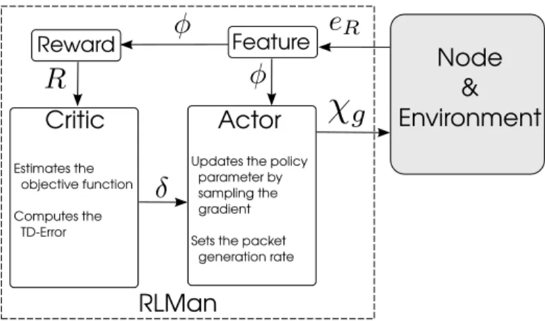
Critic
Actor
RewardNode
&
Environment
FeatureRLMan
Estimates the objective function Computes the TD-ErrorUpdates the policy parameter by sampling the gradient
Sets the packet generation rate
Fig. 2: Global architecture of RLMan.
In RL, it is assumed that all goals can be described by the maximization of expected cumulative reward. Formally, the problem is formulated as an MDP xS, A, T , Ry, detailed below.
1) The set of states S: The state of a node at time slot k
is defined by the current residual energy er. Therefore, S “
rErf ail, Emaxr s.
2) The set of actions A: An action corresponds to setting
the packet rate χg at which packets are sent. Therefore, A “
rXmin, Xmaxs.
3) The transition function T : The transition function gives
the probability of a transition to errk ` 1s when action χg
is performed in state errks. The transition function models
the dynamics of the MDP, which is in the case of energy management the energy dynamics of the node, related to both the platform and its environment.
4) The reward function R: The reward is computed as a
function of both χg and er:
R “ φχg, (11)
where φ is the feature, which corresponds to the normalized residual energy: φ “ er´ E f ail r Emax r ´ E f ail r . (12)
Therefore, maximizing the reward involves maximizing both the packet rate and the state of charge of the energy storage device. However, because the residual energy depends on the consumed energy and the harvested energy, and as these variables are stochastic, the reward function is defined by:
Rper, χgq “ E rRrk ` 1s | Srks “ er, Arks “ χgs . (13)
Energy management can be seen as a multiple reward functions system, in which both the normalized residual energy φ and
the packet rate χg need to be maximized. These two rewards
are combined by multiplication to form a single reward and to reduce to a single reward system. Other approaches to combine multiple rewards exist [11], [12].
B. Derivation of RLman
An RL agent uses its experience to evaluate a given policy by estimating its value function, a process referred to as policy evaluation. Using the value function, the policy is optimized such as the long-term obtained reward is maximized, a process called policy improvement. The EM scheme proposed in this work is an actor-critic algorithm, a class of RL techniques well-known for being capable to search for optimal policies using low variance gradient estimates [13]. This class of algorithms requires storing both a representation of the value function and the policy in memory, as opposite to other techniques such as critic-only or actor-only methods, which require only storing the value function or the policy respectively. Critic-only schemes require at each step deriving the policy from the value function, e.g., using a greedy method. However, this involves solving an optimization problem at each step, which may be computationally intensive, especially in the case of continuous action space and when the algorithm needs to be implemented on limited resource hardware, such as WSN nodes. On the other hand, actor-only methods work with a parameterized family of policies over which optimization procedure can be directly used, and a range of continuous actions can be generated. However, these methods suffer from high variance, and therefore slow learning [13]. Actor-critic methods combine actor-only and Actor-critic-only methods by storing both a parameterized representation of the policy and a value function.
Figure 2 shows the relation between the actor and the critic.
The actor updates a parameterized policy πψ, where ψ is the
policy parameter, by gradient ascent on the objective function J defined in (3). A fundamental result for computing the gradient of J is given by the policy gradient theorem [14]:
5ψJ pπψq “ ż S ρπψperq ż A Qπψpe r, χgq 5ψπψpχg | erqdχgder “ E „ Qπψpe r, χgq 5ψlog πψpχg | erq ˇ ˇ ˇ ˇ ρπψ, πψ . (14) This result reduces the computation of the performance objec-tive gradient to an expectation, and allows deriving algorithms by forming sample-based estimates of this expectation. In this
work, a Gaussian policy is used to generate χg:
πψpχg | eRq “ 1 σ?2πexp ˜ ´pχg´ µq 2 2σ2 ¸ , (15)
where σ is fixed and controls the amount of exploration, and µ is linear with the feature:
µ “ ψφ. (16)
Defining µ as a linear function of the feature enables minimal memory footprint as only one floating value, ψ, needs to be stored. Moreover, the computational overhead is also minimal
as 5ψµ “ φ, leading to:
5ψlog πψpχg | erq “
pχg´ µq
σ2 φ. (17)
It is important to notice that other ways of computing µ from the feature can be used, e.g., artificial neural networks, in which case ψ is a vector of parameters (the weights of the neural network). However, these approaches incur higher memory usage and computational overhead, and might thus not be suited to WSN nodes.
Using the policy gradient theorem as formulated in (14) may lead to high variance and slow convergence [13]. A way to reduce the variance is to rewrite the policy gradient theorem
using the advantage function Aπψpe
r, χgq “ Qπψ ´ Vπψ.
Indeed, it can be shown that [14]:
5ψJ pπψq “ E „ Aπψpe r, χgq 5ψlog πψpχg | erq ˇ ˇ ˇ ˇ ρπψ, πψ . (18) This can reduce the variance, without changing the expectation. Moreover, the TD-Error (Temporal Difference-Error), defined by:
δ “ Rrk ` 1s ` γVπψpe
rrk ` 1sq ´ Vπψperrksq, (19)
is an unbiased estimate of the advantage function, and therefore can be used to compute the policy gradient [13]:
5ψJ pπψq “ E „ δ 5ψlog πψpχg | erq ˇ ˇ ˇ ˇ ρπψ, πψ . (20)
Algorithm 1 Reinforcement learning based energy manager.
Input: errks, Rrks 1: φrks “ errks´E f ail r Emax r ´E f ail r Ź Feature (12) 2: δrks “ Rrks ` γθrk ´ 1sφrks ´ θrk ´ 1sφrk ´ 1s Ź TD Error (19), (21)
3: Ź Critic: update the value function estimate (22), (23):
4: νrks “ γλνrk ´ 1s ` φrks
5: θrks “ θrk ´ 1s ` αδrksνrks
6: Ź Actor: updating the policy (16), (17), (20):
7: ψrks “ ψrk ´ 1s ` βδrkspf rk´1s´ψrk´1sφrk´1sqσ2 φrk ´ 1s
8: Clamp µtto rXmin, Xmaxs
9: Ź Generating a new action:
10: χgrks „ N pψrksφrks, σq
11: Clamp χgrks to rXmin, Xmaxs
12: return χgrks
The TD-Error can be intuitively interpreted as a critic of the previously taken action. Indeed, a positive TD-Error suggests that this action should be selected more often, while a negative TD-Error suggests the opposite. The critic computes the TD-Error (19), and, to do so, requires the knowledge of
the value function Vπψ. As the state space is continuous,
storing the value function for each state is not possible, and therefore function approximation is used to estimate the value function. Similarly to what was done for µ (16), linear function approximation was chosen to estimate the value function, as
it requires very few computational overhead and memory:
Vθperq “ θφ, (21)
where φ is the feature (12), and θ is the approximator param-eter.
The critic, which estimates the value function by updating the parameter θ, is therefore responsible for performing policy evaluation. A well-known category of algorithms for policy evaluation are TD based methods, and in this work, the TD(λ) algorithm [15] is used:
νrks “ γλνrk ´ 1s ` φrks (22)
θrks “ θrk ´ 1s ` αδrksνrks (23)
where α P r0, 1s is a step-size parameter.
Algorithm 1 shows the proposed EM scheme. It can be seen that the algorithm has low memory footprint and incurs low computational overhead, and therefore is suitable for execution on WSN nodes. At each run, the algorithm is fed with the
current residual energy errks and the reward Rrks computed
using (11). First, the feature and the TD-Error are computed (lines 1 and 2), and then the critic is updated using the TD(λ) algorithm (lines 4 and 5). Next, the actor is updated using the policy gradient theorem at line 7, where β P r0, 1s is a step-size parameter. The expectancy of the Gaussian policy is clamped to the range of allowed values at line 8. Finally, a frequency is generated using the Gaussian policy at line 10, which will be used in the current time slot. As the Gaussian distribution is unbounded, it is required to clamp the generated value to the allowed range (line 11).
V. EVALUATION OFRLMAN
RLMan was evaluated using exhaustive simulations. This section starts by presenting the simulation setup. Then, the impact of the different parameters required by RLMan is explored. Finally, the results of the comparison of RLMan to three state-of-the-art EMs are exposed.
A. Simulation setup
The platform parameters used in the simulations correspond to PowWow [16], a modular WSN platform designed for energy harvesting. The PowWow platform uses a capacitor as energy storage device, with a maximum voltage of 5.2 V and a failure voltage of 2.8 V. The harvested energy was simulated by two energy traces from real measurements: one lasting 270 days corresponding to indoor light [17] and the other lasting 180 days corresponding to outdoor wind [18], allowing the evaluation of the EM schemes for two different energy source types. The task of the node consists in acquiring data by sensing, performing computation and then sending the data to a sink. However, in practice, the amount of energy consumed by one execution of this task varies, e.g., due to multiple retransmissions. Therefore, the amount of energy required to run one execution was simulated by a random variable
denoted by EC which follows a beta distribution. The mode
of the distribution was set to the energy consumed if only one
transmission attempt is required, denoted by ECtyp, and which
All ECtyp 8.672 mJ ECmax 36.0 mJ Xmin 1 300Hz Xmax 5 Hz T 60 s RLMan α 0.1 β 0.01 σ 0.1 γ 0.9 λ 0.9 P-FREEN [8] BOF L 0.95E max R η 1.0 Fuzzyman [9] K 1.0 η 1.0
EBeds XminT Etypc EminB XminT Etypc EstrongH XmaxT Etyp c Eweak H XminT Etypc LQ-Tracker [7] µ 0.001 B˚ 0.70Emax R α 0.5 β 1.0
TABLE I: Parameter values used for simulations. For details about the parameters of P-FREEN, Fuzzyman and LQ-Tracker, the reader can refer to the respective literature.
is considered as the typical case. The highest value that ECcan
take, denoted by ECmax, is set to the energy consumed if five
transmission attempts are necessary. The standard deviation of
EC is denoted by σC, and the ratio of σC to EtypC is denoted
by ξ:
ξ “ σC
ECtyp. (24)
Intuitively, ξ measures the variability of EC compared to its
typical value.
Three metrics were used to evaluate the EMs: the dead ratio, which is defined as the ratio of the duration the node spent in the power outage state to the total simulation duration, the
average packet rate denoted by ¯χg, and the energy efficiency
denoted by ζ and defined by: ζ “ 1 ´ ř teW,t eR,0` ř teH,t , (25)
where eR,0 is the initial residual energy, eW,t is the energy
wasted by saturation of the energy storage device during the
tthtime slot, i.e., the energy that could not be stored because
the energy storage device was full, and eH,t is the energy
harvested during the tthtime slot. Table I shows the values of
EtypC and ECmax, as well as the parameter values used when
10−3 10−2 10−1 100 σ 0.0 0.2 0.4 0.6 0.8 1.0 Dea d rat io
(a) Impact of σ on the dead ratio (λ “ 0.9, γ “ 0.9).
10−3 10−2 10−1 100 γ 0.0 0.2 0.4 0.6 0.8 1.0 Dea d rat io
(b) Impact of γ on the dead ratio (λ “ 0.9, σ “ 0.1).
10−3 10−2 10−1 100 σ 0 50 100 150 200 250 300 ¯χg (pkts per minut e) 10−1 100 1.0 1.5
(c) Impact of σ on the average packet rate (λ “ 0.9, γ “ 0.9).
10−3 10−2 10−1 100 γ 0 50 100 150 200 250 300 ¯χg (pkts per minut e) 0.1 0.3 0.5 0.7 0.9 0.75 1.00 1.25 1.50
(d) Impact of γ on the average packet rate (λ “ 0.9, σ “ 0.1).
10−3 10−2 10−1 100 σ 0.9980 0.9985 0.9990 0.9995 1.0000 ζ
(e) Impact of σ on the efficiency (λ “ 0.9, γ “ 0.9).
10−3 10−2 10−1 100 γ 0.99970 0.99975 0.99980 0.99985 0.99990 0.99995 1.00000 ζ 0.1 0.3 0.5 0.7 0.9 0.000090 0.000095 0.000100 +9.999×10⁻¹
(f) Impact of γ on the efficiency (λ “ 0.9, σ “ 0.1).
Fig. 3: Impact of the parameters on the performance of RLMan using indoor light energy harvesting.
B. Tuning RLMan
RLMan requires three parameters to be set: the discount factor γ, the trace decay parameter λ and the policy standard deviation σ. Using the setup previously introduced, the impact of these parameters on the performance of the proposed scheme was explored, and the results are shown in Fig. 3. For each value of a parameter, one hundred simulations were run, each performed using different seeds for the random number generators. The capacitance was set to 1 F, as it is the value used by the PowWow platform [16] that was simulated, leading to Erf ail « 3.9 J and Emaxr « 13.5 J.. Each cross in Fig. 3
represents the result of one simulation run, while the dots show the average of all the simulation runs for one value of a parameter. The results show that λ does not significantly impact the performance of RLMan, and therefore the results regarding this parameter are not exposed. Simulations were performed for both indoor light and outdoor wind energy traces, but as the obtained results are similar for both cases, only the results of indoor light are shown.
a) Impact ofσ: This parameter is the standard deviation
of the Gaussian policy, and therefore controls the amount of exploration performed by the agent. Fig. 3a exposes the impact of σ on the dead ratio. It can be seen that setting this parameter
0 5 10 15 20 25 30 Time (days) 0.0 0.2 0.4 0.6 0.8 1.0 Harvested Power (mW)
(a) Harvested power from indoor light.
0 5 10 15 20 25 30 Time (days) 0.2 0.3 0.4 0.5 0.6 0.7 0.8 0.9 1.0 Feature φ
(b) Feature (state of charge of the energy storage device).
0 5 10 15 20 25 30 Time (days) 0.00 0.01 0.02 0.03 0.04 0.05 Policy expectancy µ (Hz)
(c) Gaussian policy expectation.
0 5 10 15 20 25 30 Time (days) 0 10 20 30 40 50 Reward R (d) Reward.
Fig. 4: Behavior of the EM scheme the first 30 days.
to values less than 0.05 leads to non-null dead ratio, which can be explained in Fig. 3c, which shows that values of σ lower than 0.05 lead to too high average packet rates. On the other hand, choosing values of σ higher than 0.1 leads to energy energy waste, as illustrated in Fig. 3e. As a consequence of these results, σ was set to a value of 0.1 in the rest of this work.
b) Impact of γ: This parameter is the discount factor of
the objective function, and therefore controls how much future rewards lose their value compared to immediate rewards. It can be seen on Fig. 3b that values of γ higher than 0.9 lead to power outages. Fig. 3d shows that γ strongly impacts the average packet rate, especially when higher than 0.3. The steep increase of the average packet rate that can be seen for values of γ higher than 0.9 explains the power outages. Moreover, Fig. 3f reveals that choosing values of γ higher than 0.2 and lower than 0.9 leads to energy waste. Therefore, considering these results, γ was set to 0.9 in the rest of this work.
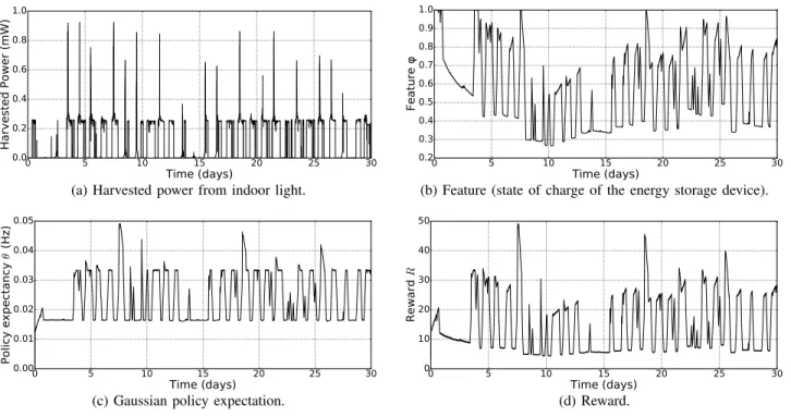
Fig. 4 shows the behavior of the proposed EM during the first 30 days of simulation using the indoor light energy trace, and with λ “ 0.9, γ “ 0.9 and σ “ 0.1. Fig. 4a shows the harvested power, and Fig. 4b shows the feature (φ), corresponding to the normalized residual energy. Fig. 4c exposes the expectancy of the Gaussian distribution used to generate the packet rate (µ), and Fig. 4d shows the reward (R), computed using (11). It can be seen that the first day the energy storage device was saturated (Fig. 4b), as the average packet rate was progressively increasing (Fig. 4c), leading to higher rewards (Fig. 4d). As during the second and third days
the amount of harvested energy was low, the residual energy dropped, causing a decrease of the rewards while the policy expectancy was stable. Starting the fourth day, energy was harvested again, enabling the node to increase its activity, as it can be seen on Fig. 4c. Finally, it can be noticed that if a lot of energy was wasted by saturation of the energy storage device the first 5 days, this is no longer true once this period of learning is over.
C. Comparison to state-of-the-art
RLMan was compared to P-FREEN, Fuzzyman, and LQ-Tracker, three state-of-the-art EM schemes that aim to maximize the packet rate. P-FREEN and Fuzzyman require the tracking of the harvested energy in addition to the residual energy, and were therefore executed with perfect knowledge of this value. RLMan and LQ-Tracker were only fed with the value of the residual energy. Both the indoor light and the wind energy traces were considered. First, the EMs were evaluated for different capacitances of the energy storage device, as it impacts the cost and form factor of the WSN nodes. Then, the EMs were compared regarding ξ, which allows us to evaluate the robustness of the algorithms regarding the variability of
EC.
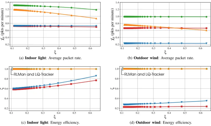
1) Impact of the capacitance of the energy storage device: The EMs were evaluated for capacitance sizes ranging from 0.5 F to 3.5 F, and for a value of ξ of 0.16. All the EMs successfully avoid power failure when powered by indoor light or outdoor wind. Fig. 5 exposes the comparison results. As it
0.5 1.0 1.5 2.0 2.5 3.0 3.5 C (F) 0.4 0.6 0.8 1.0 1.2 1.4 ¯χg (pkts per minut e)
(a) Indoor light: Average packet rate.
0.5 1.0 1.5 2.0 2.5 3.0 3.5 C (F) 0.4 0.6 0.8 1.0 1.2 1.4 ¯ χg (pkts per minut e)
(b) Outdoor wind: Average packet rate.
0.5 1.0 1.5 2.0 2.5 3.0 3.5 C (F) 0.3 0.4 0.5 0.6 0.7 0.8 0.9 1.0 ζ
RLMan and LQ-Tracker
(c) Indoor light: Energy efficiency.
0.5 1.0 1.5 2.0 2.5 3.0 3.5 C (F) 0.3 0.4 0.5 0.6 0.7 0.8 0.9 1.0 ζ
RLMan and LQ-Tracker
(d) Outdoor wind: Energy efficiency.
Fig. 5: Average packet rate and energy efficiency for different capacitance values, in the case of indoor light and outdoor wind.
can be seen on Fig 5c and Fig. 5d, both RLMan and LQ-Tracker achieve more than 99.9 % efficiency, for indoor light and outdoor wind, for all capacitance values, and despite the fact that they require only the residual energy as an input. In addition, when the node is powered by outdoor wind, RLMan always outperforms the other EMs in terms of average packet rate for all capacitance values, as shown in Fig. 5b. When the node is powered by indoor light, RLMan also outperforms all the other EMs, except LQ-Tracker when the values of the capacitance are higher than 2.8 F. Moreover, the advantage of RLMan over the other EMs is more significant for small values of the capacitance. Especially, the average packet rate is more than 20 % higher compared to LQ-Tracker in the case of indoor light, and almost 70 % higher in the case of outdoor wind, when the capacitance value is set to 0.5 F. This is encouraging as using small capacitance leads to lower cost and lower form factor.
2) Impact of the variability ofEC: The EMs were evaluated
for different values of ξ. ECtyp and Emax
C were kept constant,
while σC was changed by varying the parameters of the beta
distribution. The capacitance of the energy storage device was set to 1.0 F, as it is the value used by PowWow. Results are shown in Fig. 6. It can be seen from Fig. 6c and Fig. 6d that
in both the cases of indoor light and outdoor wind, increasing
the variability of EC does not affect the efficiency of RLMan
and LQ-Tracker, both of which achieve an efficiency of 1. Concerning Fuzzyman and P-FREEN, increasing ξ enables higher efficiencies. Indeed, P-FREEN and Fuzzyman outputs are an energy budget, from which a packet rate must be calculated. The calculation of the packet rate was performed
based on a typical cost of a task execution EtypC . However,
as ξ increases, EC tends to be higher than ECtyp more often,
which causes less energy waste as more energy is required to achieve the same quality of service.
Fig. 6a and Fig. 6b reveal that RLMan achieves higher quality of service in term of packet rate. In the case of indoor light, both packet rates decrease as ξ increases. However, the gain of RLMan over LQ-Tracker becomes more significant as ξ increases. Regarding the case of outdoor wind, the packet rate is not affected by ξ when using RLMan, but decreases when using LQ-Tracker, showing the benefits enabled by RLMan. LQ-Tracker output is a duty-cycle in the range r0, 1s, from which the packet rate must be calculated. Similarly to what was done with P-FREEN and RLMan, the typical value of
EC, E
typ
C was used for computing the packet rate from the
0.1 0.2 0.3 0.4 0.5 0.6 ξ 0.2 0.4 0.6 0.8 1.0 1.2 1.4 ¯χg (pkts per minut e)
(a) Indoor light: Average packet rate.
0.1 0.2 0.3 0.4 0.5 0.6 ξ 0.2 0.4 0.6 0.8 1.0 1.2 1.4 ¯χg (pkts per minut e)
(b) Outdoor wind: Average packet rate.
0.1 0.2 0.3 0.4 0.5 0.6 ξ 0.2 0.4 0.6 0.8 1.0 ζ
RLMan and LQ-Tracker
(c) Indoor light: Energy efficiency.
0.1 0.2 0.3 0.4 0.5 0.6 ξ 0.2 0.4 0.6 0.8 1.0 ζ
RLMan and LQ-Tracker
(d) Outdoor wind: Energy efficiency. Fig. 6: Average packet rate and energy efficiency for different values of ξ, in the case of indoor light and outdoor wind.
These results show the practical advantages of using RL-Man. RLMan does not require any knowledge on the energy consumption of the node. It successfully adapts to variations of the energy consumption of the node task (e.g., due to channel noise or sensors variability), and ensures high energy efficiency and packet rate. One can imagine that the performance of the other schemes could be increased by tracking the energy consumption of the node, and using an adaptive algorithm to compute the packet rate from the output of the EM, but this would require additional resources and increase the complexity, memory and computation footprint of the energy manager. RLMan inherently adapts to the dynamics of both the harvested energy and the consumed energy, and therefore does not require this additional complexity.
VI. CONCLUSION
The problem of designing energy management schemes for wireless sensor nodes powered by energy harvesting is tackled in this paper, and a novel algorithm based on reinforcement learning, named RLMan, is introduced. RLMan uses function approximations to achieve low memory and computational overhead, and only requires the state of charge of the en-ergy storage device as an input, which makes it suitable for
resource-constrained systems such as wireless sensor nodes and practical to implement. It was shown, using exhaustive simulations, that RLMan enables significant gains regarding packet rate compared to state of the art approaches, both in the case of indoor light and outdoor wind. Moreover, RLMan successfully adapts to variations of the consumed energy, and therefore does not require additional energy consumption tracking schemes to keep high efficiency and quality of service.
REFERENCES
[1] R. J. M. Vullers, R. v. Schaijk, H. J. Visser, J. Penders, and C. V. Hoof, “Energy Harvesting for Autonomous Wireless Sensor Networks,” IEEE Solid-State Circuits Magazine, vol. 2, no. 2, pp. 29–38, Spring 2010. [2] A. Kansal, J. Hsu, S. Zahedi, and M. B. Srivastava, “Power
Manage-ment in Energy Harvesting Sensor Networks,” ACM Transactions on Embedded Computing Systems, vol. 6, no. 4, 2007.
[3] A. Castagnetti, A. Pegatoquet, C. Belleudy, and M. Auguin, “A Frame-work for Modeling and Simulating Energy Harvesting WSN Nodes with Efficient Power Management Policies,” EURASIP Journal on Embedded Systems, no. 1, 2012.
[4] T. N. Le, A. Pegatoquet, O. Berder, and O. Sentieys, “Energy-Efficient Power Manager and MAC Protocol for Multi-Hop Wireless Sensor Networks Powered by Periodic Energy Harvesting Sources,” IEEE Sensors Journal, vol. 15, no. 12, pp. 7208–7220, 2015.
[5] F. Ait Aoudia, M. Gautier, and O. Berder, “GRAPMAN: Gradual Power Manager for Consistent Throughput of Energy Harvesting Wireless Sensor Nodes,” in IEEE 26th Annual International Symposium on Personal, Indoor, and Mobile Radio Communications (PIMRC), August 2015.
[6] R. Margolies, M. Gorlatova, J. Sarik, G. Stanje, J. Zhu, P. Miller, M. Szczodrak, B. Vigraham, L. Carloni, P. Kinget, I. Kymissis, and G. Zussman, “Energy-Harvesting Active Networked Tags (EnHANTs): Prototyping and Experimentation,” ACM Transactions on Sensor Net-works, vol. 11, no. 4, pp. 62:1–62:27, November 2015.
[7] C. M. Vigorito, D. Ganesan, and A. G. Barto, “Adaptive Control of Duty Cycling in Energy-Harvesting Wireless Sensor Networks,” in 4th Annual IEEE Communications Society Conference on Sensor, Mesh and Ad Hoc Communications and Networks (SECON), June 2007. [8] S. Peng and C. P. Low, “Prediction free energy neutral power
manage-ment for energy harvesting wireless sensor nodes,” Ad Hoc Networks, vol. 13, Part B, 2014.
[9] F. Ait Aoudia, M. Gautier, and O. Berder, “Fuzzy power management for energy harvesting Wireless Sensor Nodes,” in IEEE International Conference on Communications (ICC), May 2016.
[10] R. C. Hsu, C. T. Liu, and H. L. Wang, “A Reinforcement Learning-Based ToD Provisioning Dynamic Power Management for Sustainable Operation of Energy Harvesting Wireless Sensor Node,” IEEE Trans-actions on Emerging Topics in Computing, vol. 2, no. 2, pp. 181–191, June 2014.
[11] C. Liu, X. Xu, and D. Hu, “Multiobjective Reinforcement Learning: A Comprehensive Overview,” IEEE Transactions on Systems, Man, and
Cybernetics: Systems, vol. 45, no. 3, pp. 385–398, March 2015. [12] C. R. Shelton, “Balancing Multiple Sources of Reward in Reinforcement
Learning,” in Advances in Neural Information Processing Systems 13, T. K. Leen, T. G. Dietterich, and V. Tresp, Eds. MIT Press, 2001, pp. 1082–1088. [Online]. Available: http://papers.nips.cc/paper/ 1831-balancing-multiple-sources-of-reward-in-reinforcement-learning. pdf
[13] I. Grondman, L. Busoniu, G. A. D. Lopes, and R. Babuska, “A Survey of Actor-Critic Reinforcement Learning: Standard and Natural Policy Gradients,” IEEE Transactions on Systems, Man, and Cybernetics, Part C (Applications and Reviews), vol. 42, no. 6, pp. 1291–1307, November 2012.
[14] R. S. Sutton, D. A. McAllester, S. P. Singh, and Y. Mansour, “Policy Gradient Methods for Reinforcement Learning with Function Approx-imation.” in Advances in Neural Information Processing Systems 12, vol. 99, 2000, pp. 1057–1063.
[15] R. S. Sutton, “Learning to Predict by the Methods of Temporal Differences,” Machine Learning, vol. 3, no. 1, pp. 9–44, 1988. [16] O. Berder and O. Sentieys, “PowWow: Power Optimized
Hard-ware/Software Framework for Wireless Motes,” in International Con-ference on Architecture of Computing Systems (ARCS), February 2010. [17] M. Gorlatova, A. Wallwater, and G. Zussman, “Networking Low-Power Energy Harvesting Devices: Measurements and Algorithms,” in IEEE INFOCOM, April 2011.
[18] “National Renewable Energy Laboratory (NREL),” http://www.nrel.gov/.