Sequential beat-to-beat P and T wave delineation and waveform estimation in ECG signals: Block Gibbs sampler and marginalized particle filter

HAL Id: hal-01117225

https://hal.archives-ouvertes.fr/hal-01117225

Submitted on 16 Feb 2015

HAL is a multi-disciplinary open access

archive for the deposit and dissemination of

sci-entific research documents, whether they are

pub-lished or not. The documents may come from

teaching and research institutions in France or

abroad, or from public or private research centers.

L’archive ouverte pluridisciplinaire HAL, est

destinée au dépôt et à la diffusion de documents

scientifiques de niveau recherche, publiés ou non,

émanant des établissements d’enseignement et de

recherche français ou étrangers, des laboratoires

publics ou privés.

Sequential beat-to-beat P and T wave delineation and

waveform estimation in ECG signals: Block Gibbs

sampler and marginalized particle filter

Chao Lin, Georg Kail, Audrey Giremus, Corinne Mailhes, Jean-Yves

Tourneret, Franz Hlawatsch

To cite this version:

Chao Lin, Georg Kail, Audrey Giremus, Corinne Mailhes, Jean-Yves Tourneret, et al..

Sequen-tial beat-to-beat P and T wave delineation and waveform estimation in ECG signals:

Block

Gibbs sampler and marginalized particle filter. Signal Processing, Elsevier, 2014, 104, pp.174-187.

�10.1016/j.sigpro.2014.03.011�. �hal-01117225�

!

"

"##

!

#

$% " &'&()

" % $ "&* &*&+#, -

(*&. *' *&&

/ "

"## 0

-#&* &*&+#, -

(*&. *' *&&

"

1 2

3

1 4

-

4

1

5

1 2

1 6

!7

8

1 9

:

! (*&.

-

;

-1

&*.

&<.!&=< $

>

*&+?!&+=.

Sequential beat-to-beat P and T wave delineation and

waveform estimation in ECG signals: Block Gibbs sampler

and marginalized particle filter

$

Chao Lin

a

, Georg Kail

b

, Audrey Giremus

c

, Corinne Mailhes

a,n

,

Jean-Yves Tourneret

a

, Franz Hlawatsch

b

a_{IRIT/ENSEEIHT/TeSA, University of Toulouse, Toulouse, France}

b_{Institute of Telecommunications, Vienna University of Technology, Vienna, Austria} c_{IMS-LAPS-UMR 5218, University of Bordeaux, Talence, France}

Keywords:

ECG P and T wave delineation Bayesian inference

Beat-to-beat analysis

Sequential Monte Carlo methods Gibbs sampling

Marginalized particle filter

a b s t r a c t

For ECG interpretation, the detection and delineation of P and T waves are challenging tasks. This paper proposes sequential Bayesian methods for simultaneous detection, threshold-free delineation, and waveform estimation of P and T waves on a beat-to-beat basis. By contrast to state-of-the-art methods that process multiple-beat signal blocks, the proposed Bayesian methods account for beat-to-beat waveform variations by sequentially estimating the waveforms for each beat. Our methods are based on Bayesian signal models that take into account previous beats as prior information. To estimate the unknown parameters of these Bayesian models, we first propose a block Gibbs sampler that exhibits fast convergence in spite of the strong local dependencies in the ECG signal. Then, in order to take into account all the information contained in the past rather than considering only one previous beat, a sequential Monte Carlo method is presented, with a marginalized particle filter that efficiently estimates the unknown parameters of the dynamic model. Both methods are evaluated on the annotated QT database and observed to achieve significant improvements in detection rate and delineation accuracy compared to state-of-the-art methods, thus providing promising approaches for sequential P and T wave analysis.

1. Introduction

The electrocardiogram (ECG) represents the electrical activity of the heart, which corresponds to repetitions of a cardiac cycle, i.e., a heartbeat. Each beat consists of a QRS complex surrounded by P and T waves that are associated with the mechanical phases occurring during a cardiac cycle. Most of the clinically useful information can be derived from the wave intervals, amplitudes, and morphology. Therefore, the development of efficient and robust methods for auto-matic ECG delineation (determining the locations of the peaks and boundaries of the individual waves) has become a major

http://dx.doi.org/10.1016/j.sigpro.2014.03.011

☆_{This work was supported in part by the Austrian Science Fund (FWF)}

under grant S10603 and by a grant of Saint Jude Med. that was awarded within the project Dynbrain funded by STIC AmSud. Parts of this work were previously presented at EUSIPCO 2012, Bucharest, Romania, August 2012.

n

Corresponding author.

E-mail addresses:chao.lin@tesa.prd.fr(C. Lin), georg.kail@nt.tuwien.ac.at(G. Kail),

audrey.giremus@ims-bordeaux.fr(A. Giremus), corinne.mailhes@enseeiht.fr(C. Mailhes), jean-yves.tourneret@enseeiht.fr(J.-Y. Tourneret), franz.hlawatsch@tuwien.ac.at(F. Hlawatsch).

challenge for the biomedical signal processing community. Among the ECG waves, the QRS complex is relatively easy to detect and is thus generally used as a reference within the cardiac cycle. For P and T wave detection and delineation, most algorithms perform QRS detection first and then define temporal search windows before and after the QRS location points in which they assume the P and T waves are located. Subsequently, an appropriate strategy is used to enhance the distinctive features of each wave in order to locate the wave peaks and boundaries.

In the last two decades, a variety of techniques have been proposed for automatically detecting and delineating P and T waves [1–8]. These techniques are based on adaptive filtering[1], low-pass differentiation[2], wavelet transform[3,4], action potential models[5], pattern recog-nition [6], extended Kalman filters [7], or evolutionary optimization [8]. However, because of the low slope and amplitude of the P and T waves as well as the presence of noise, interference, and baseline fluctuation, P and T wave detection and delineation remain challenging tasks. Furthermore, in addition to the locations of the wave peaks and boundaries, the shapes and amplitudes of P and T waves have also been shown to contain important information about numerous pathologies[9].

A Bayesian model was recently proposed to simulta-neously solve the P and T wave delineation and waveform estimation problems [10,11]. This model was based on prior distributions for the unknown parameters (wave locations and amplitudes [10] as well as waveform and local baseline coefficients [11]). Several Gibbs-type sam-plers were then proposed to estimate the model para-meters. However, the Bayesian model of[10,11]relied on a non-overlapped multiple-beat processing window. More precisely, the shapes of the P and T waves within a multiple-beat processing window were assumed to be equal, whereas their amplitudes and locations were allowed to vary from one beat to another. Due to the pseudo-cyclostationary nature of the ECG signal, the P and T waveforms in a given beat are usually similar but not

exactly equal to those of the adjacent beats. Therefore, the

performance of P and T wave delineation can be expected to improve if the waveforms are estimated in a

beat-to-beat manner that allows for temporal variations of

wave-form morphology across the beats. A beat-to-beat proces-sing mode is also advantageous for an on-line operation with reduced memory requirements and rapid adaptation to changing signal characteristics.

In this paper, we present and study Bayesian methods that enable simultaneous P and T wave delineation and waveform estimation on a to-beat basis. First, a beat-to-beat Bayesian model is proposed which modifies the multiple-beat-window-based model studied in[10,11]by introducing dependencies among waveform coefficients. Instead of assigning a white Gaussian prior to the temporal sequence of waveform coefficients, we use a prior “with memory” that depends on the estimates of the previous beat. A Gibbs sampler with a block constraint, referred to as block Gibbs sampler (BGS), is then used for estimating the parameters of the resulting beat-to-beat model. Simula-tion results show that the proposed sequential model and processing improve the convergence behavior of the

samplers proposed in [10,11] as well as the accuracy of estimating the locations, amplitudes, and shapes of the P and T waves. The improved convergence behavior can be explained by a considerable reduction of the parameter dimension, since only one beat is processed at any time instant instead of multiple beats.

In the second part of this paper, we present a sequential Monte Carlo method that takes into account all the information contained in the past rather than only that of the previous beat. The principle of this method is to exploit the sequential nature of the ECG signal by defining an appropriate dynamic model. This model adapts to the morphology variations across the ECG beats by using a random walk model for the waveform coefficients. A particle filter is then employed to estimate the unknown parameters of the proposed model. Despite the simplicity of the particle filter principle, its main drawback is its computational complexity, especially for a large state dimen-sion. In practice, if the state dimension is high, many random samples are necessary to achieve a good accuracy of the estimates. However, this problem can be alleviated for non-linear models containing a subset of parameters which are linear and Gaussian, conditional upon the other parameters. In this case, using the technique of Rao-Blackwellization[12]or marginalization [13], the linear/Gaussian parameters can be optimally estimated through standard linear Gaussian filter-ing. In our case, the state equations are linear with respect to a subset of the unknown parameters. Thus, we propose to use a marginalized particle filter (MPF) that generates particles in the space of the “nonlinear” parameters and runs one Kalman filter for each of these particles to estimate the “linear” parameters. A comparison between the proposed sequential BGS, the proposed MPF, and state-of-the-art methods shows that both of the proposed methods provide significant improvements in terms of estimation performance for the locations, amplitudes, and shapes of the P and T waves. Moreover, the MPF method typically exhibits a better perfor-mance than the BGS method for estimating the shapes of the P and T waveforms, at the price of a higher computational complexity.

The paper is organized as follows.Section 2describes the proposed beat-to-beat Bayesian model for the non-QRS signal components and a BGS that generates samples distributed according to the posterior of this Bayesian model.Section 3 presents a dynamic model based on the proposed beat-to-beat Bayesian framework and an associated MPF. The detec-tors and estimadetec-tors used for P and T wave detection, estima-tion, and delineation are discussed in Section 4. Section 5 reports the results of numerical simulations performed on the standard annotated QT database[14]. These results allow the performance of the two proposed methods to be compared with that of state-of-the-art algorithms. Finally, Section 6 presents conclusions and suggests future work.

2. Beat-to-beat Bayesian model and block Gibbs sampler

2.1. Signal model for one non-QRS interval

It is common to partition ECGs into QRS complexes and non-QRS intervals. Non-QRS intervals are located between the end of a QRS complex and the subsequent QRS onset,

and they potentially contain P and T waves. In this paper, we assume that the locations of the non-QRS intervals have been determined by a preliminary QRS detection step using, e.g., the Pan–Tompkins algorithm [15], and that baseline wanderings have been removed by, e.g., the median filtering technique proposed in[16]. As shown in Fig. 1, the non-QRS interval Jn associated with the nth

beat consists of two complementary subintervals: a T search interval JT;n, which may contain a T wave, and a

P search interval JP;n, which may contain a P wave. The

temporal lengths of the intervals Jn, JT;n, and JP;n will

be denoted by Nn, NT;n, and NP;n, respectively. Note that

NT;nþ NP;n¼ Nn. The lengths NT;n and NP;n can be

deter-mined by a cardiologist or simply as fixed percentages of

Nn. In this work, we choose NT;n¼ NP;n¼ Nn=2 for

simpli-city. Our goal is to estimate the locations, amplitudes, and shapes of the P and T waves within their respective search intervals J_T;nand J_P;n. Note that only the locations of the wave peaks are constrained to lie within their respective search intervals.

2.1.1. Convolution model

The baseline-free signal in the non-QRS interval Jncan be

approximated by two pulses representing the P and T waves (see Fig. 1). Similar to the blind deconvolution problem in [17,18], the T wave is modeled by the convolution of an unknown binary “indicator sequence” bT;n¼ ðbT;n;1…

bT;n;NT;nÞ

T _{indicating the wave locations (b}

T;n;k¼ 1 if there is

a wave at the kth possible location, b_T;n;k¼ 0 otherwise) with an unknown T waveform hT;n¼ ðhT;n; % L…hT;n;LÞT. Analogous

definitions for the P wave yield bP;n¼ ðbP;n;1…bP;n;NP;nÞ

T _and

h_{P;n¼ ðhP;n; % L⋯ hP;n;LÞ}T_{. Here, the waveform length 2L þ 1 is}

chosen as a fixed percentage of Nn that is large enough to accommodate the actual supports of the P and T waves. Within each indicator vector b_T;nand b_P;n, at most one entry is nonzero because at most one wave may occur in any given search interval. According to this model, the nth non-QRS signal component can be expressed as follows:

x_n;k¼ ∑ NT;n j ¼ 1 h_{T;n;k % j}bT;n;jþ ∑ Nn j ¼ NT;nþ 1 h_{P;n;k % j}bP;n;j % NT;nþ en;k ð1Þ with k AJn¼ f1; …; Nng: Here, en;k denotes white Gaussian

noise with unknown variance s2

e;n. Furthermore, we have set

h_T;n;k¼ h_P;n;k¼ 0 for k=2 f % L; …; Lg.

2.1.2. Waveform expansion

Following[19,20], we represent the P and T waveforms by a basis expansion using discrete-time versions of Hermite functions. Thus, the waveform vectors can be written as

h_{T;n¼ HαT;n;} h_{P;n¼ HαP;n ð2Þ} where H is a ð2L þ 1Þ ) G matrix whose columns are the first G Hermite functions (with Gr 2L þ1), suitably sampled and truncated to length 2L þ 1, and αT;n and αP;n

are unknown coefficient vectors of length G. By using these expansions, the number of unknown parameters can be significantly reduced (from 2L þ 1 to G for each wave-form). More specifically, the ECG signals involved in our study were sampled with a sampling frequency of 250 Hz. Considering a heart rate of around 60 beats per minute, that makes on average 250 samples for each beat. We used 20 Hermite coefficients for each P and T wave plus two wave location parameters and one noise variation para-meter. Thus, the ratio between the number of parameters to be estimated and the available data (used for the estimation) is approximately 0.2. Note that the amplitudes of the P and T waves are absorbed into the coefficient vectors α_T;nand α_P;n. This is a difference from the model in [10,11], where the amplitudes were defined for each beat individually whereas the P and T waveforms were fixed for multiple beats.

2.1.3. Vector formulation

Using (2), we obtain the following vector representa-tion of the non-QRS signal in(1):

x_{n¼ BT;nHαT;nþ BP;nHαP;nþ en ð3Þ} where xn¼ ðxn;1…xn;NnÞ

T_{, B}

T;n is the Nn) ð2L þ 1Þ Toeplitz

matrix with first row ðbT;n;L þ 1…bT;n;1 0 … 0Þ and first

col-umn ðb_{T;n;L þ 1}…bT;n;NT;n 0… 0Þ

T_{, B}

P;n is the Nn) ð2L þ 1Þ

Toeplitz matrix with last row ð0 … 0 b_P;n;NP;n…_bP;n;N P;n% LÞ and last column ð0 … 0 b_P;n;1…_bP;n;N

P;n% LÞ

T_{, and e}

n¼ ðen;1…

en;NnÞ

T _{is a Gaussian vector with zero mean and covariance}

matrix s2

e;nINn, with INn denoting the identity matrix of size Nn) Nn.

2.2. Likelihood function, prior, and posterior

According to the parametrization introduced inSection 2.1, the unknown parameters for the nth non-QRS interval Jn are given by the random vector θn9ðbTT;nb

T P;nαTT;n

αT_P;ns2

e;nÞ

T_{. Note, in particular, that the noise variance s}2 e;n

may vary from one beat to another. Bayesian detection/ estimation relies on the posterior distribution, pðθnjxnÞ p

pðxnjθnÞpðθnÞ, where p means “equal up to a positive

factor that does not depend on θn,” pðxnjθnÞ is the

like-lihood function, and pðθnÞ is the prior distribution of θn.

The next two subsections present the likelihood function and priors considered in this study.

2.2.1. Likelihood function

Using (3)and the fact that e_n;k is white and Gaussian with variance s2

e;n, the likelihood function (viewed as Fig. 1. Signal model for the beat-to-beat processing scheme.

a function of xn) is obtained as

pðxnjθnÞ ¼ N ðBT;nHαT;nþ BP;nHαP;n; s2e;nINnÞ ð4Þ

where N ðμ; CÞ denotes the multivariate Gaussian probabil-ity densprobabil-ity function with mean vector μ and covariance matrix C.

2.2.2. Prior distributions

Wave indicators: The indicators b_T;n;k are subject to a

block constraint: within JT;n, there is one T wave (thus1,

JbT;nJ ¼ 1) or none (thus, JbT;nJ ¼ 0), the latter case being

very unlikely. Therefore, we define the prior of b_T;n as

pðbT;nÞ ¼ p0 if JbT;nJ ¼ 0 p1 if JbT;nJ ¼ 1 0 otherwise 8 > < > : ð5Þ

where p1¼ ð1 % p0Þ=NT;n and p0 is chosen very small. Similarly, within JP;n, there is one P wave or none;

there-fore, the prior of b_P;nis defined as in(5), with p₁¼ ð1 % p0Þ=

NP;n. The wave indicator vectors bT;n and bP;nfor different

search intervals (i.e., different values of n) are assumed to be statistically independent.

Waveform coefficients: The waveform coefficient vectors

αT;nand αP;nfor the nth non-QRS interval Jnare supposed

to depend on the respective coefficient vectors in the ðn % 1Þth non-QRS interval Jn % 1. Consider the T wave as

an example. The prior of αT;n is defined as

pðαT;njbT;n; αT;n % 1Þ ¼

δðαT;n% αT;n % 1Þ if JbT;nJ ¼ 0

N ðαT;n % 1; s2αIGÞ if JbT;nJ ¼ 1

(

ð6Þ where δð+Þ is the Dirac delta function. For the variance s2

α, we choose a value that yields a reasonable variability of

the waveform coefficients from one interval to another. Note that when there is no T wave in the search interval ( JbT;nJ ¼ 0), the prior sets αT;n equal to αT;n % 1, i.e., the

waveform coefficients are equal to those in the previous interval JT;n % 1. The prior of the P waveform coefficient

vector αP;n is defined in an analogous way, with αT;n % 1

replaced by α_{P;n % 1}. These definitions of the priors of α_T;n and α_P;n introduce a memory in the statistical model for the P and T waveforms and, in turn, induce a sequential processing.

Noise variances: The noise variances s2

e;n are modeled as

independent random variables distributed according to an inverse gamma distribution pðs2

e;nÞ ¼ IGðξ; ηÞ, where ξ and η

are fixed hyperparameters defining a vague prior (as in[21]). We note at this point that the Gaussian priors of αT;n

and αP;n are conjugate priors with respect to the Gaussian

likelihood function (4), i.e., the resulting full conditional distributions (required in the Gibbs sampler) are also Gaussian [22, p. 97]. A similar remark applies to the inverse gamma prior of s2

e;n. The choice of conjugate priors

yields a considerable simplification of our detection/esti-mation algorithm.

Joint prior: Since there are no known relations between

ðbT;n; αT;nÞ, ðbP;n; αP;nÞ, and s2e;n, all these sets of parameters

are assumed to be a priori statistically independent. There-fore, the joint prior for the total parameter vector

θn¼ ðbT_T;nbT_P;nαT_T;nαT_P;ns2

e;nÞT factors as

pðθnjαT;n % 1; αP;n % 1Þ ¼ pðαT;njbT;n; αT;n % 1Þ pðbT;nÞ

)pðαP;njbP;n; αP;n % 1Þ pðbP;nÞ pðs2e;nÞ: ð7Þ

2.2.3. Posterior distribution

The posterior distribution of the parameter vector θnis

obtained by using Bayes' rule, i.e.,

pðθnjxn; αT;n % 1; αP;n % 1Þ p pðxnjθnÞpðθnjαT;n % 1; αP;n % 1Þ ð8Þ

where the right-hand term can be further expressed and factored using (4) and (7). Because the proposed method works sequentially and all estimates from the previous beat are available, we can substitute the estimates ^α_{T;n % 1} and ^α_{P;n % 1} for α_{T;n % 1} and α_{P;n % 1} in pðθnjxn; αT;n % 1; αP;n % 1Þ

when estimating θnbased on(8). Due to the complexity of

the posterior distribution, we propose to use a Monte Carlo (sample-based) detection/estimation method. More speci-fically, we propose a BGS that generates samples asymp-totically distributed according to pðθnjx; ^αT;n % 1; ^αP;n % 1Þ (see

Section 2.3). From these samples, the discrete parameters b_T;n and b_P;n are then detected by means of the sample-based maximum a posteriori (MAP) detector, and the continuous parameters αT;n, αP;n, and s2e;n are estimated

by means of the sample-based minimum mean square error (MMSE) estimator, as described inSection 4.

2.3. Block Gibbs sampler for beat-to-beat wave extraction

The proposed BGS for the nth non-QRS interval Jn is

summarized inAlgorithm 1. Note that the interval index

n is omitted for all parameters to simplify the notation,

while the index n% 1 is kept to avoid any ambiguity. The term “block Gibbs sampler” is used to reflect the block constraints related to the wave indicator vectors bT

and bP, which are encompassed in the corresponding

priors (see (5)). To see that Algorithm 1 is a valid Gibbs sampler, note that the sampling steps for bT and

αT are equivalent to jointly sampling bT and αT from

pðbT; αTjbP; ^αT;n % 1; αP; s2e; xÞ, and similarly for bP and αP.

Closed-form expressions of the sampling distributions used in Algorithm 1 are presented and derived in the technical report[23].

Algorithm 1. Block Gibbs sampler.

Sample bTfrom pðbTjbP; ^αT;n % 1; αP; s2e; xÞ Sample αTfrom pðαTjbT; bP; ^αT;n % 1; αP; s2e; xÞ Sample bPfrom pðbPjbT; ^αP;n % 1; αT; s2e; xÞ Sample αPfrom pðαPjbT; bP; ^αP;n % 1; αT; s2e; xÞ Sample se 2 from pðs2 ejbT; bP; αT; αP; xÞ

3. Dynamic beat-to-beat Bayesian model and marginalized particle filter

Section 2presented a beat-to-beat Bayesian model that describes dependencies among waveform coefficients. A prior “with memory” (depending on the previous esti-mates of the P and T waveforms) was assigned to the current beat. In this section, elaborating on [24], an MPF method [25] is proposed to take into account all the 1

information contained in the past of the current beat to be

processed. First, we present a dynamic model as a basis for performing simultaneously P and T wave delineation and waveform estimation on a beat-to-beat basis. This dynamic model is similar to the Bayesian model intro-duced inSection 2. However, it adapts to the morphology variations across the ECG beats by using a random walk model for the waveform coefficients. Then, following the sequential Monte Carlo principle, an MPF is used to estimate the unknown parameters of the proposed model. The idea is to generate particles only for the states appearing nonlinearly in the dynamics and run one Kal-man filter for each of these particles to estimate the “linear” parameters.

3.1. Dynamic signal model for non-QRS intervals

As in Section 2, we assume that the locations of the non-QRS intervals have been determined and baseline wanderings have been removed by a preprocessing stage. The signal model is the same as inSection 2.1, except for the following two differences.

First, the model(1)is split into its T and P parts:

xn;k¼ ∑ NT;n j ¼ 1 hT;n;k % jbT;n;jþ en;k; k A JT;n¼ f1; …; NT;ng ð9Þ xn;k¼ ∑ NP;n j ¼ 1 hP;n;k % j % NT;nbP;n;jþ en;k; k AJP;n¼ fNT;nþ 1; …; Nng: ð10Þ Using (2), we obtain the following representation of the signal vector xT;n¼ ðxn;1⋯xn;NT;nÞ

T _{corresponding to the T}

wave interval in(9):

x_T;n¼B~_{T;nHαT;nþ eT;n ð11Þ} where ~B_T;ncomprises the first N_T;nrows of B_T;ndefined in Section 2.1.3. A similar representation can be obtained for the signal vector xP;n¼ ðxn;NT;nþ 1⋯xn;NnÞ

T _{corresponding to}

the P wave interval in(10)using ~B_{P;n, which comprises the} last NP;n rows of BP;n.

Second, the variance of the noise e_n;k has not been included in the parameter vector (as in the proposed BGS) since it would increase significantly the computational com-plexity of the algorithm. In our simulations, the noise variance was estimated in a preprocessing step using the BGS (although other methods could be used as well). Thus, e_T;n¼ ðe_n;1… _en;N

T;nÞ

T _{and e}

P;n¼ ðen;NT;nþ 1…en;NnÞ

T _are

Gaus-sian vectors with zero mean and covariance matrix s2 eINT;nand s2

eINP;n, respectively, s

2

e being the estimated noise variance.

3.2. Likelihood function, posterior, and prior

Using the modified signal model from Section 3.1, the likelihood function—now taking into account all beat indices up to n—factors as pðx1:njθ0:nÞ ¼ pðxT;1:njbT;0:n; αT;0:nÞ pðxP;1:njbP;0:n; αP;0:nÞ: ð12Þ Here, e.g., x1:n9ðxT1…xTnÞ T _{and θ} 0:n9ðθT0…θTnÞ T_{. As before}

(cf.Section 2.2.2), we assume that the T wave parameters are independent of the P wave parameters. Therefore,

using(12), the joint posterior distribution can be written

pðθ0:njx1:nÞ p pðbT;0:n; αT;0:njxT;1:nÞpðbP;0:n; αP;0:njxP;1:nÞ:

This allows us to split the estimation problem into two independent problems related to the P and T waves. In the following, only the T wave dynamic model and estimation problem are discussed, and the subscript T is omitted for notational convenience.

Due to the parametrization(11), the state vector for the

nth T wave interval is given by θn¼ ðbTn αTnÞ

T_{. Note that θ} nis

now short for θT;n, and thus different from the θnused, e.g.,

inSection 2.2. For the indicator vector bn, we use the prior

in (5) with p0¼ p1¼ 1=ðNT;nþ 1Þ. This prior is a uniform

distribution on the set of all possible bnsuch that JbnJ ¼ 1

or JbnJ ¼ 0. Indicator vectors bn for different beat indices

n are assumed to be statistically independent. Since the

ECG waveforms are usually similar for two consecutive beats, we propose to assign a random walk prior to the T waveform coefficient vector αn, i.e.,

αn¼ αn % 1þ vn % 1 ð13Þ

where αn % 1denotes the T waveform coefficient vector of the

ðn % 1Þth beat and the vectors vn, N 0; s& 2αIG' are statistically

independent (of each other and of α0:n) additive white

Gaussian noise vectors. This leads to the conditional prior

pðαnjαn % 1Þ ¼ N ðαn % 1; s2αIGÞ, which is the same as in the

second case of (6). Note that here, in contrast to (6), the coefficient vector changes even if JbnJ ¼ 0. The variance s2α

depends on how fast the waveform coefficients are expected to change with time. Since the non-QRS components are normalized by dividing by the amplitude of the respective R peak, we have to account for possible significant variations of the waveforms with time. We therefore propose to use a large value of s2

α, which corresponds to a non-informative

condi-tional prior of αn. Note that the value of s2α can be further

adjusted by an expert or by calculating the ECG waveform variance of an example ECG segment in an off-line parameter selection procedure as in [26]. Because of (13) and the independence of vn for different n as well as of α0:n, the

waveform coefficient vector αn is conditionally independent,

given αn % 1, of all previous coefficient vectors α0:n % 2, i.e.,

pðαnjα0:n % 1Þ ¼ pðαnjαn % 1Þ.

3.3. A marginalized particle filter for beat-to-beat wave analysis

Our goal is to estimate jointly the discrete-valued indicator vector bn and the waveform vector αn, i.e., to

estimate the state vector θn. In a Bayesian framework, all

inference is based on the posterior distribution of the unknown parameters given the set of available observa-tions, expressed as pðθ0:njx1:nÞ. Particle filters (PFs) are a

class of methods well-suited to perform the estimation of the hybrid state vector θ0:n. They approximate the target

distribution by an empirical distribution ^ pðθ0:njx1:nÞ ¼ ∑ Ns i ¼ 1 wðiÞ nδðθ0:n% θðiÞ0:nÞ; where ∑ Ns i ¼ 1 wðiÞ n ¼ 1:

The weights wðiÞ

n and the particles θðiÞ0:n are classically

obtained by sequential importance sampling and a selec-tion (resampling) step to prevent degeneracy[25].

3.3.1. Development of the MPF

While the classical PFs are fairly easy to implement, a main drawback is that, in practice, the required number of particles increases quickly with the state dimension. The MPF can reduce the number of parameters estimated by the PF and therefore allows fewer particles to be used. More specifi-cally, the MPF takes advantage of linear Gaussian sub-structures in the state parameters θnto decrease the variance

of the state estimates. The key idea is to split θninto two parts

θL_n and θNL

n , where θ L

n denotes the state parameters with

conditionally linear dynamics and θNL_n denotes the nonlinear state parameters. We can then marginalize out θL_n and generate particles distributed according to pðθNL

n jx1:nÞ using

a PF. The particles are finally used to compute the MAP estimator of θNL

n . In parallel, each particle is associated with a

Kalman filter (KF) that computes recursively the mean and covariance matrix of the Gaussian distribution pðθL_njθNL_n ; x1:nÞ.

It can be observed from (11) that both the discrete vector bnand the continuous vector αnenter linearly in the

observation xn, given the respective other parameter. Since

only continuous parameters can be handled by the KF, we choose θL

n¼ αn and θNLn ¼ bn.The KF and the PF correspond

to two factors of the joint posterior according to the following factorization: pðb0:n; α0:njx1:nÞ ¼ pðα0:njb0:n; x1:nÞ |fflfflfflfflfflfflfflfflfflfflfflfflffl{zfflfflfflfflfflfflfflfflfflfflfflfflffl} KF pðb0:njx1:nÞ |fflfflfflfflfflfflfflffl{zfflfflfflfflfflfflfflffl} PF : ð14Þ

The marginal distribution of the discrete parameters is approximated by ^ pðb0:njx1:nÞ ¼ ∑ Ns i ¼ 1 wðiÞ nδ½b0:n% bðiÞ0:n. ð15Þ

where Nsis the number of particles and δ[.] denotes the discrete-time unit sample. Then, by inserting(15)in (14) and summing out b0:n, the posterior distribution of the

continuous parameters can be approximated by ^ pðα0:njx1:nÞ ¼ ∑ Ns i ¼ 1 wðiÞ npðα0:njbðiÞ0:n; x1:nÞ: ð16Þ

Integrating out α0:n % 1yields

^ pðαnjx1:nÞ ¼ ∑ Ns i ¼ 1 wðiÞ npðαnjbðiÞ0:n; x1:nÞ: ð17Þ

It can be shown that pðα0:njbðiÞ0:n; x1:nÞ in(16)and pðαnjbðiÞ0:n;

x_{1:nÞ in(17) are Gaussian. Therefore,(16) and (17)} repre-sent mixtures of Gaussian distributions. Note that one KF is associated with each particle bðiÞ_0:nwith i ¼ 1; …; Ns.

Further-more, in practice, only the marginal distribution ^pðαnjx1:nÞ

is updated (rather than ^pðα0:njx1:nÞ). The MPF recursions

are summarized inAlgorithm 2, presented for the T wave case. The different steps involved in this algorithm are detailed in the rest of this section.

Algorithm 2. Marginalized particle filter.

fInitializationg for i ¼ 1; …; Nsdo

Set bðiÞ

0 ¼ 0NT;n)1, P

ðiÞ

0 ¼ 0G)G, and wðiÞ0 ¼ 1, and choose a suitable initialization of the waveform coefficients ^αðiÞ₀ (seeSection 5.1.1). end for

fTime recursiong for n ¼ 1; 2; … do

for i ¼ 1; …; Nsdo

fKF and PF propagationg KF prediction for αðiÞ

n (see (18)) Sample bðiÞ

n , Prðbn¼ βkjb ðiÞ

0:n % 1; x1:nÞ (see(19)) KF correction for αðiÞ

n (see (20)) Calculate weights (see (21) and (22))

~ wðiÞ n ¼ w ðiÞ n % 1∑k A JT;npðxnjb ðiÞ n ¼ βk; bðiÞ0:n % 1; x1:n % 1ÞPrðbðiÞn ¼ βkÞ end for fWeight normalizationg for i ¼ 1; …; Nsdo wðiÞn ¼ ~wðiÞn=∑ Ns j ¼ 1w~ ðjÞ n end for fState estimationg

Estimate bnand αn(see (23)) fParticle resamplingg Calculate ^N_eff¼ 1=∑Ns i ¼ 1ðw ðiÞ nÞ2 if_N^ effr0:7 + Nsthen

Resample using systematic sampling scheme[25, p. 11] end if

end for

3.3.2. Kalman filter prediction

At time n, the previous MMSE state estimate is ^αðiÞ n % 1¼

Efαn % 1jx1:n % 1; bðiÞ0:n % 1g and its covariance matrix is P ðiÞ n % 1¼

Covfαn % 1jx1:n % 1; bðiÞ0:n % 1g. We define the predicted state

vector _α^ðiÞ

njn % 19Efαnjx1:n % 1; b ðiÞ

0:n % 1g and its covariance

PðiÞ

njn % 19Covfαnjx1:n % 1; bðiÞ0:n % 1g. Using(13), it can be shown

that the prediction step of the KF can be written as ^

αðiÞ_{njn % 1}¼ ^αðiÞ_{n % 1}; PðiÞ njn % 1¼ P

ðiÞ n % 1þ s

2

αIG: ð18Þ

Note that the predicted state vector and its covariance computed by the KF, ^αðiÞ

njn % 1 and P ðiÞ

njn % 1, will be directly

used to propagate the particles and compute their impor-tance weights, as explained presently (see(20)).

3.3.3. Importance distribution for the indicators

It is well known that the choice of the importance distribution is a critical issue in the design of efficient PF algorithms. To generate samples in relevant regions of the state space, i.e., corresponding to a high likelihood pðxnjθnÞ,

a natural strategy consists of taking into account informa-tion from the most recent observainforma-tions xn. The importance

distribution that is optimal in the sense that it minimizes the variance of the importance weights is qðbnjbðiÞ0:n % 1;

x_{1:nÞ ¼ pðbnjb}ðiÞ

0:n % 1; x1:nÞ[27]. Thus, the optimal importance

distribution for bn is obtained as

Prðbn¼ βkjbðiÞ0:n % 1; x1:nÞ p pðxnjbn¼ βk; bðiÞ0:n % 1; x1:n % 1ÞPrðbn¼ βkÞ ð19Þ

where β_k for k AJ_T;n¼ f1; …; NT;ng is an NT;n) 1 vector

whose kth entry is 1 and all remaining entries are zero. Note that β0 is the all-zero vector, which represents the

case where there is no T wave. It can be shown that, for b_{0:ngiven, α0:nand x1:nare jointly Gaussian. It follows that} the distribution pðxnjbn¼ βk; b

ðiÞ

0:n % 1; x1:n % 1Þ in (19) is a

Gaussian one. According to(11), its mean ^xðiÞ_n;k and covar-iance matrix SðiÞ

n;kcan be computed from the KF prediction

(18)as follows: ^ xðiÞ n;k¼ ~ B n;kH ^α ðiÞ njn % 1 SðiÞ n;k¼ ~ B n;kHP ðiÞ njn % 1H T_B~T n;kþ s 2 eINT;n

where ~B

n;k is the matrix ~Bn that corresponds to bn¼ βk.

Note that contrary to the standard PF, the importance distribution for the indicators no longer depends on the coefficient vector α0:n, which has been marginalized out.

On the other hand, it depends on the past sequence b0:n % 1.

3.3.4. Kalman filter correction

After receiving the observation xn for beat index n,

the predicted waveform coefficients ^αðiÞ

njn%1can be updated

for each generated wave indicator particle bðiÞ

n. The KF

correction procedure can be written as SðiÞ n ¼ ~ BðiÞ nHP ðiÞ njn % 1H T ðB~ðiÞ nÞ T þ s2_eINT;n ð20aÞ KðiÞ n ¼ P ðiÞ njn % 1H T ðB~ðiÞ nÞ T ðSðiÞ_nÞ% 1 ð20bÞ ^ αðiÞn ¼ ^α ðiÞ njn % 1þ K ðiÞ nðxn%B~ ðiÞ nH ^α ðiÞ njn % 1Þ ð20cÞ

PðiÞ_n ¼ ðIG% KðiÞnB~ ðiÞ nHÞP

ðiÞ

njn % 1 ð20dÞ

where ~BðiÞ

n is the matrix ~Bn that corresponds to bn¼ bðiÞn .

3.3.5. PF weight computation

When the optimal importance distribution is used to propagate the particles, the weights satisfy the following recursion: wðiÞ n pw ðiÞ n % 1pðxnjx1:n % 1; b ðiÞ 0:n % 1Þ: ð21Þ

Here, pðxnjx1:n % 1; bðiÞ0:n % 1Þ is the normalization constant of

(19), i.e., pðxnjx1:n % 1; bðiÞ0:n % 1Þ ¼ ∑ k A JT;n pðxnjbðiÞn ¼ βk; b ðiÞ 0:n % 1; x1:n % 1ÞPrðbðiÞn ¼ βkÞ: ð22Þ

4. P and T wave detection, estimation, and delineation In this section, we discuss sample-based wave detec-tion, parameter estimadetec-tion, and wave delineation for the two proposed methods.

4.1. Block Gibbs sampler

We will denote by S 9fbðiÞ T; b ðiÞ P; α ðiÞ T; α ðiÞ P; s 2ðiÞ e g Ns i ¼ 1 the set

of samples produced by our BGS after a burn-in period. (The burn-in period is the initial period of sampler itera-tions during which the sampler converges; the samples produced by the sampler during the burn-in period are not used for detection/estimation[28, p. 5].)

For detecting and locating P and T waves, we use the following sample-based blockwise MAP detector for the wave indicators bT and bP:

^ b_{T¼ arg max} i A f1;…;Nsg pSðb ðiÞ TÞ; ^ b_{P¼ arg max} i A f1;…;Nsg pSðb ðiÞ PÞ:

Here, pSðbTÞ is a sample-based approximation of the

posterior probability pðbTjx; ^αT;n % 1; ^αP;n % 1Þ. More

specifi-cally, pSðbTÞ is defined as the number of samples bðiÞT in S

that equal the respective value of bT, normalized by the

total number of samples, Ns. Analogous considerations

apply to pSðbPÞ.

The detection step described above is followed by sample-based estimation of the waveform coefficients αT

and αP and of the noise variance s2e. Let us combine these parameters into the parameter vector θ,b9ðαTT αTP s2_eÞT. Furthermore, we define the set I as the set of sample indices i Af1; …; Nsg such that bðiÞT ¼

^

b_{T and b}ðiÞ

P ¼

^ b_{P. To} estimate θ,b, we use the sample mean

^ θ,b¼ 1 jI ji A I∑ θðiÞ_,b where θðiÞ ,b9ðα ðiÞT T α ðiÞT P s 2ðiÞ

e ÞTand jI j denotes the number of

elements in I . This can be interpreted as a sample-based approximation of the MMSE estimator (note that the MMSE estimator is given by the posterior mean Efθ,bjx; bT; bP; ^αT;n % 1; ^αP;n % 1g). Thus, θ^,b depends on

^ b_T, ^

b_{P, ^α}

T;n % 1, and ^αP;n % 1.

The final step is wave delineation (localization of the peaks and boundaries of the P and T waves). Because of the convolution model (1), our detection/estimation problem is affected by a time-shift ambiguity [17,29]. Following [17], we resolve this ambiguity by performing an appro-priate time shift after generating the waveform samples in the block Gibbs sampler. This time shift ensures that the maximum of the waveform is located at the center k ¼ 0 of the waveform support interval f% L; …; Lg and, thus, the location of a nonzero detected indicatorb^_T;k¼ 1 orb^_P;k¼ 1 directly indicates the peak of the respective T or P wave. A detailed description of an algorithm for resolving the time-shift ambiguity is also provided in[29].

It is broadly accepted that the turning points defined by the largest local maximum of the curvature of the estimated waveform on each side of the detected wave peak are good estimates of the wave boundaries[6,30]. The curvature of the estimated T waveformh^_T;k is defined as[6]

κ_T;k9 ^

h″_T;k

½1 þ ðh^0_T;kÞ2.3=2

; k A f %L; …; Lg

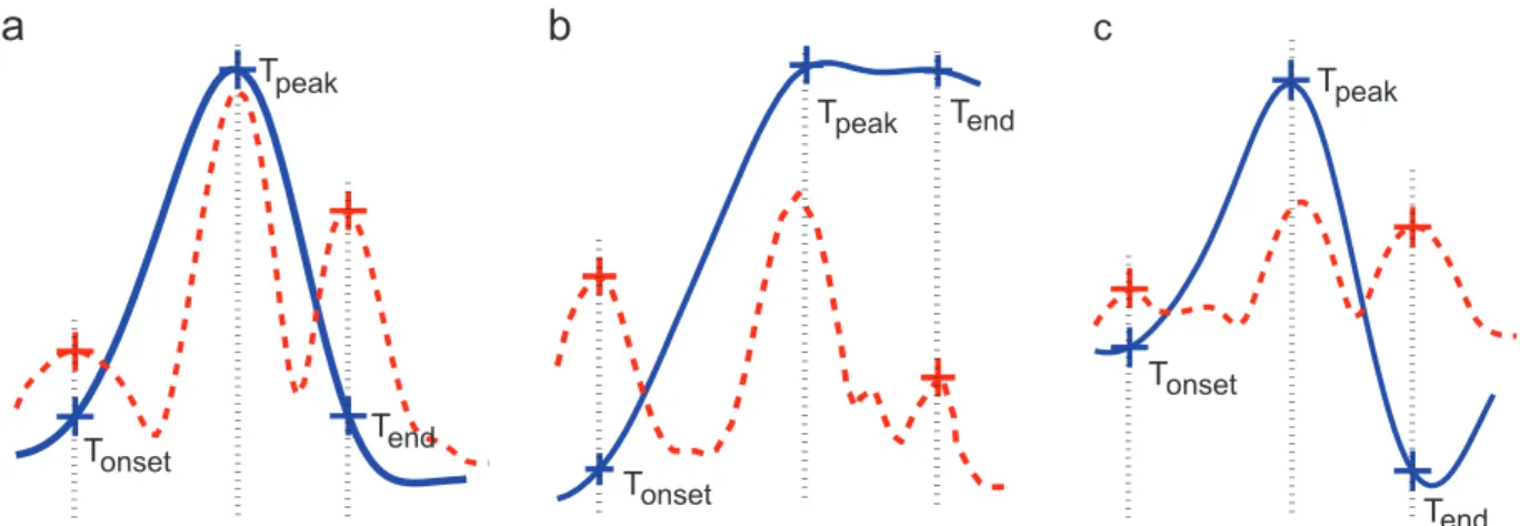
where h^0_T;k and h^″_T;k are discrete-time counterparts of the first and second derivatives (e.g., h^0_T;k is defined as the differenceh^_T;k%h^_{T;k % 1}). Using the turning points for deli-neation avoids the use of rigid detection and delideli-neation thresholds. Fig. 2 illustrates the method by showing the delineation results obtained for three different T wave morphologies. Simulation results for the proposed BGS will be presented inSection 5.

4.2. Marginalized particle filter

In the MPF, the sample-based blockwise MAP estimator is used for estimating the binary sequence bn, while the

sample-based MMSE estimator is used for estimating the waveform coefficients αn: ^ b_{n¼ arg max} i A f1;…;Nsg ^ pðbðiÞ_njx1:nÞ; α^n¼ ∑ Ns i ¼ 1 wðiÞ nα^ ðiÞ n: ð23Þ Here, ^pðbðiÞ

njx1:nÞ is obtained by marginalizing (15) and the

estimate ^αnis the mean of the Gaussian mixture(17)with ^αðiÞn

The wave delineation consists of determining the peaks and boundaries of the detected P and T waves. As mentioned in Section 4.1, because the time-shift ambi-guity is removed, the nonzero wave indicator estimated by the MPF directly indicates the center of the corre-sponding waveform time window. Thus, the peak of the respective T or P wave is indicated by the location of the maximum of the estimated waveform. Furthermore, the wave boundaries can be located by applying the delinea-tion criterion described in Section 4.1 to the estimated waveforms.

5. Simulation results

5.1. Simulation setup

Both of the proposed Bayesian wave detection/estima-tion/delineation methods were evaluated on the QT database (QTDB), which was previously used in several other studies [14]. The QTDB provides a reference for validating automatic wave-boundary estimation meth-ods. It is a two-channel database containing cardiologist annotations for at least 30 beats per dataset for both channels. It includes 105 datasets from the widely used MIT-BIH arrhythmia database, the European ST-T data-base, and some other well-known databases. The cardiol-ogist annotations of the QTDB were performed using two leads, whereas the proposed delineation methods work on a single-channel basis. To compare the single-channel delineation results produced by our methods with the manual annotations of the QTDB, we chose for each T or P wave the channel where the detected wave peak location was closer to the annotated one (as suggested in[4,30]). In a preprocessing step, the QRS complexes were detected and the borders of the non-QRS intervals Jn were

determined using the Pan–Tompkins algorithm [15]. (The same preprocessing step was performed in[10,11].) In another preprocessing step, baseline wanderings were removed. P and T search intervals J_T;nand J_P;nwere then defined as the first and second half of Jn. Both of the

proposed methods sequentially process one non-QRS interval Jn after another.

5.1.1. BGS setup

For each non-QRS interval Jn, the BGS generated 100

samples according to the conditional distributions speci-fied in Algorithm 1. The first 40 samples constituted the burn-in period, and the remaining 60 were used for detection/estimation (thus, Ns¼ 60). The fixed

hyperpara-meters involved in the prior distributions were chosen as

p0¼ 0:01, s2α¼ 0:01, ξ ¼ 11, and η ¼ 0:5; these values allow

for an appropriate waveform variability from one beat to another and provide a noninformative prior for the noise variance s2

e;n. Note that the non-QRS components were

normalized using the corresponding R peak values to handle different amplitude resolutions. For the first non-QRS interval (n ¼ 1), the previous waveform coefficient estimates ^α_T;0and ^α_P;0were initialized with the coefficient vector α for which h is closest to the 2L þ 1 Hann window [31], with an amplitude equal to half the R peak amplitude. The waveform length was chosen as 2L þ1 ¼ Nn=3, which

is large enough to accommodate the actual support of the T or P wave.

Because the proposed beat-to-beat BGS method pro-cesses only one non-QRS interval at any given time, both its memory requirements and its computational complex-ity are smaller than those of the window-based method of [10]. For instance, for the proposed method using 100 sampler iterations, the processing time per beat is approxi-mately 0.3 s using a nonoptimized MATLAB implementation running on a 3.0-GHz Pentium IV computer, compared to about 2 s for the method of[10]. Note that this computation time could be further reduced by developing implementa-tions on digital signal processors.

5.1.2. MPF setup

In the MPF method, the fixed hyperparameters involved in the prior distributions were chosen as s2

α¼ 0:01 and

s2_e¼ 0:1. The chosen value of s2

α allows for an appropriate

waveform variability from one beat to another. The chosen value of se

2

was obtained from a previous estimation of the noise level, using the mean value estimated by the BGS method, but could be taken from any other noise estimator. The non-QRS components were again normalized using the corresponding R peak values to handle different amplitude

T_peak T_onset Tend T_peak Tpeak T_onset T_onset Tend T_end

Fig. 2. Delineation results obtained for three different T wave morphologies. Solid blue line: estimated T waveform, dotted red line: corresponding curvature. The crosses indicate the estimated peak and boundary locations. (a) Normal sinus T wave from QT database (QTDB)[14]dataset sel17453 channel 1; (b) ascending T wave from QTDB sele0203 channel 1; (c) biphasic T wave from QTDB sele0603 channel 1. (For interpretation of the references to color in this figure caption, the reader is referred to the web version of this article.)

resolutions. The waveform vectorh^_{0¼ H ^α0 was initialized} as in the BGS method.

An important issue with PF methods is the number of particles. Using the estimated parameters, we recon-structed the non-QRS part of the signal (based on the noiseless parts of models(9) and (10)) and compared it to the original signal non-QRS part. This allowed us to compute a normalized mean square error (NMSE) to assess the quality of the estimation. Table 1 shows the NMSE versus the number of particles Ns. As can be seen, benefit-ing from the optimal importance distribution derived in Section 3.3.3, good estimation performance can be

obtained with a moderate number of particles. We chose

Ns¼ 200 particles for all the following simulations in order

to guarantee an NMSE close to % 40 dB. For the MPF method using 200 particles, the processing time per beat is approximately 0.5 s using a nonoptimized MATLAB implementation running on a 3.0-GHz Pentium IV computer.

5.2. Qualitative analysis

In this section, we first show the posterior distributions as well as estimation and delineation results obtained by the proposed beat-to-beat BGS method on a typical example. Then, we present a qualitative comparison of the proposed BGS and MPF methods with state-of-the-art methods on several representative ECG segments.

Fig. 3(a) shows two consecutive beats from the QTDB dataset sele0136. The corresponding sample-based esti-mates of the marginal posterior probabilities of having a T

Table 1

Normalized mean square error (NMSE) versus number of particles used in the MPF method.

Ns 10 50 100 200 300

NMSE (dB) % 25 % 31 % 34 % 40 % 42

Fig. 3. Simulation results obtained with the proposed BGS method. (a) Two consecutive beats from QTDB dataset sele0136; (b) estimated marginal posteriors PSðbk¼ 1Þ; (c) estimated P and T waveforms (dotted red line) compared with the original P and T waveforms (blue) and delineation results. (For interpretation of the references to color in this figure caption, the reader is referred to the web version of this article.)

or P wave at a given location k, PSðbT;n;k¼ 1Þ and

PSðbP;n;k¼ 1Þ, are depicted in Fig. 3(b). (For k AJT,

PSðbk¼ 1Þ equals the probability PSðbTÞ of the specific

hypothesis bT that contains a 1-entry at location k, and

similarly for k AJP.) Fig. 3(c) shows the actual P and T

waveforms and their estimates obtained by the proposed BGS method for each search interval, along with the corresponding delineation results (i.e., the estimated wave onsets, peaks, and ends, which were determined as described inSection 4). One can observe noticeable differ-ences between the two consecutive T waveforms (at time instants 4.92 s and 6.10 s), as well as between the two consecutive P waveforms (at time instants 5.64 s and 6.83 s). This confirms the pseudo-cyclostationary nature of the ECG signal and justifies our introduction of a beat-to-beat processing scheme that allows for beat-beat-to-beat variations of the P and T waveforms. The results displayed inFig. 3(c) show that the BGS algorithm is able to estimate these P and T waveforms with good accuracy.

Next, we present a qualitative comparison of the proposed BGS and MPF methods with the multi-beat

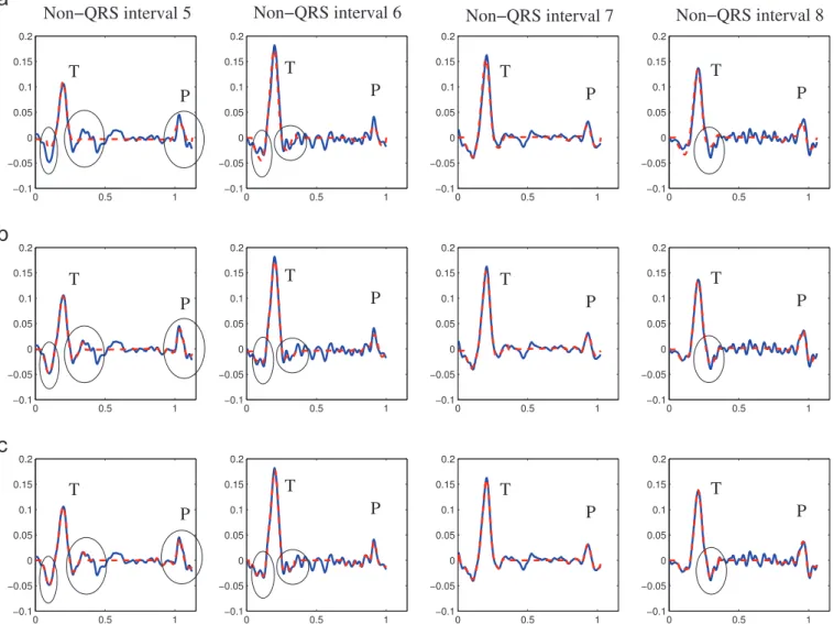
method of [10] (based on a partially collapsed Gibbs sampler (PCGS)) to highlight the benefits of beat-to-beat processing. To evaluate the methods under real physiolo-gical noise conditions, we added muscular activity noise from the MIT-BIH noise stress test database. The estimated non-QRS signal components obtained with the different methods are displayed inFigs. 4and5for eight successive beats of a segment of QTDB dataset sele0136. The original ECG signal is also shown for comparison. It can be seen that the proposed beat-to-beat methods (BGS and MPF) provide closer agreements with the original ECG signal when compared to the multi-beat method, especially at the onsets and ends of the waves, which is a desirable property for wave delineation. These results show that, contrary to the multi-beat method of[10], the beat-to-beat BGS and MPF methods are able to capture the changes affecting the P and T waveforms. Additional results are available in a technical report [23]. In particular, both proposed methods are compared with the method of [7] (which is based on an extended Kalman filter) and are shown to be able to handle specific pathologies such as

Fig. 4. Four consecutive segments from QTDB dataset sele0136 (blue) superimposed with their reconstructions using the estimated parameters (dotted red). (a) PCGS multi-beat method of[10]; (b) proposed beat-to-beat BGS method; (c) proposed beat-to-beat MPF method. (For interpretation of the references to color in this figure caption, the reader is referred to the web version of this article.)

premature ventricular contractions, a pathology in which parts of the T waves are crossing the interval border and the P waves are missing.

5.3. Quantitative analysis

Next, we provide a quantitative performance comparison of the two proposed methods with the multi-beat method of [10] and three alternative methods [2,4,5], based on an exhaustive evaluation performed on the entire QTDB. For a quantitative analysis of the performance of P and T wave detection, as in[2,4,5,10,11], we computed the sensitivity (also referred to as detection rate) Se ¼ TP=ðTPþFNÞ and the positive

predictivity Pþ_{¼ TP=ðTP þ FPÞ, where TP denotes the number}

of true positive detections (wave was present and was detected), FN stands for the number of false negative detec-tions (wave was present but was missed), and FP for the number of false positive detections (wave was not present but was detected). The performance of wave delineation was measured by the average (denoted as m) and standard deviation (denoted as s) of the time differences between the

results of the considered method and the corresponding cardiologist annotations. The indicated time values (in ms) are based on a sampling frequency of 250 Hz. The quantities

m and s were computed separately for the wave onset times tP;on and tT;on, the wave peak times tP;peak and tT;peak, and the

wave end times t_P;endand t_T;end. We note that while the QTDB includes annotations made by two cardiologists, we consid-ered only those of the first cardiologist, who provided annotations for at least 30 beats per dataset.

Table 2shows the results for Se, Pþ_{, and m7 s obtained}

for the entire QTDB. It can be seen that the two proposed methods detect the P and T waves annotated by the cardiologist with high sensitivity: the sensitivity Se is 100% for the T waves and 99.93% or 99.95% for the P waves. Similarly good results were obtained for the posi-tive predictivity Pþ_{, which is between 98.01% and 99.30%}

for the T waves and 99.10% or 99.23% for the P waves. Both the Se values and the Pþ _{values are typically better than}

those obtained with the other methods, including the recently proposed multi-beat method of [10]. Regarding the delineation performance, it is seen fromTable 2that

Fig. 5. Four other consecutive segments from QTDB dataset sele0136 (blue) superimposed with their reconstructions using the estimated parameters (dotted red). (a) PCGS multi-beat method of[10]; (b) proposed beat-to-beat BGS method; (c) proposed beat-to-beat MPF method. (For interpretation of the references to color in this figure caption, the reader is referred to the web version of this article.)

the two proposed methods delineate the annotated P and T waves with mean errors jmj not exceeding 4 ms (except for

tT;on) and with smaller standard deviations s than the other

methods (with two exceptions). We note that delineation error tolerances have been recommended by the CSE Working Party [32]. In particular, the standard deviation s for t_P;on,

tP;end, and tT;endshould be at most 2sCSE, which is listed in the

last row of Table 2. However, a stricter recommendation proposed in[4]is s rsCSE. According toTable 2, the standard

deviations for t_P;endachieved by both proposed methods and the standard deviation for tP;onachieved by the proposed MPF

method comply with the loose recommendation. For the t_T;end results, both proposed methods comply with the strict recommendation. InTable 2, the advantage of the proposed beat-to-beat methods over the multi-beat method of[10] is not as clear as inFigs. 4and5. This is because only a small part of the signals evaluated inTable 2exhibit obvious inter-beat waveform variations. FromTable 2, it is furthermore seen that the detection and delineation results obtained with the two proposed methods are quite similar.

To further appreciate the differences between the two proposed methods, we conducted a quantitative compar-ison of their waveform estimation performance. First, in order to constitute our ground truth, we visually selected from the MIT-BIH Normal Sinus Rhythm Database 20 segments of ECG signals, each of duration 10 s, with a high SNR and no significant arrhythmia. Then, to generate

realistic ECG signals, the ground truth was corrupted by adding muscular activity noise from the MIT-BIH noise stress test database with an SNR ranging from 20 to

Table 2

Comparison of the detection and delineation performance of the proposed beat-to-beat BGS and MPF methods with that of the PCGS multi-beat method of [10], the wavelet transform based method of[4](WT), the low-pass differentiation based method of[2](LPD), and the action potential based method of[5]. The variances of these methods are compared with the delineation error tolerance of[32], which is provided in the last row. (N/A: not available).

Method Parameters tP;on tP;peak tP;end tT;on tT;peak tT;end

Beat-to-beat BGS (proposed) Annotations 3176 3176 3176 1345 3403 3403

Se (%) 99.93 99.93 99.93 100 100 100

Pþ _{(%) 99.10 99.10 99.10 98.01 99.30 99.30}

m7 s (ms) 3.4714.2 1.175.3 % 2.1 7 9.8 6.8716.3 % 0.8 7 4.1 % 3.1 7 14.0

Beat-to-beat MPF (proposed) Annotations 3176 3176 3176 1345 3403 3403

Se (%) 99.95 99.95 99.95 100 100 100

Pþ _{(%) 99.23 99.23 99.23 98.67 99.20 99.20}

m7 s (ms) 3.178.3 1.275.3 2.779.8 6.5716.3 % 0.4 7 4.8 % 3.8 7 14.2

Multi-beat partially collapsed Gibbs sampler[10] Annotations 3176 3176 3176 1345 3403 3403

Se (%) 99.60 99.60 99.60 100 100 100 Pþ _{(%) 98.04 98.04 98.04 97.23 99.15 99.15} m7 s (ms) 1.7710.8 2.778.1 2.5711.2 5.7716.5 0.779.6 2.7713.5 WT[4] Annotations 3194 3194 3194 N/A 3542 3542 Se (%) 98.87 98.87 98.75 N/A 99.77 99.77 Pþ _{(%) 91.03 91.03 91.03 N/A 97.79 97.79} m7 s (ms) 2.0714.8 3.6713.2 1.9712.8 N/A 0.2713.9 % 1.6 7 18.1

LPD[2] Annotations N/A N/A N/A N/A N/A N/A

Se (%) 97.70 97.70 97.70 N/A 99.00 99.00

Pþ _{(%) 91.17 91.17 91.17 N/A 97.74 97.74}

m7 s (ms) 14.0713.3 4.8710.6 % 0.1 7 12.3 N/A % 7.2 7 14.3 13.5727.0

Action potential based method[5] Annotations N/A N/A N/A N/A N/A N/A

Se (%) N/A N/A N/A N/A 92.60 92.60

Pþ _{(%) N/A N/A N/A N/A N/A N/A}

m7 s (ms) N/A N/A N/A 20.9729.6 % 12.0 7 23.4 0.8730.3

Delineation error tolerance 2sCSE(ms) 10.2 N/A 12.7 N/A N/A 30.6

Fig. 6. Waveform estimation SNR improvement measure SNRimpobtained with the proposed MPF and BGS methods and the multi-beat PCGS method of[10]versus the input SNR for 20 signal segments selected from the MIT-BIH Normal Sinus Rhythm database and corrupted by muscular activity noise.

% 5 dB. For a quantitative evaluation, we considered the SNR improvement measure defined as

SNRimp¼ 10 log Jx %c J 2

Jz %c J2 !

where x is the noisy signal, c is the clean signal, and z is the estimated signal. This evaluation was carried out only on the non-QRS intervals (P and T waveforms) of each signal. In order to obtain a fair performance comparison between the different algorithms, 20 Monte Carlo runs of each method were considered for each ECG signal seg-ment. The output SNR was averaged over the 400 results for each input SNR (20 runs for each of the 20 signal segments). InFig. 6, the means and standard deviations of the SNR improvement SNRimpare plotted versus the input

SNR. It can be observed that the proposed BGS and MPF algorithms clearly outperform the PCGS method [10] in terms of SNR improvement. Furthermore, the MPF algo-rithm outperforms the BGS algoalgo-rithm.

6. Conclusion

This paper presented and studied two Bayesian methods for beat-to-beat P and T wave delineation and waveform estimation. Instead of using a processing window that con-tains several successive beats involving the same P and T waveforms by assumption, the proposed methods account for beat-to-beat variations of the P and T waveforms by proces-sing individual beats sequentially (i.e., with memory). First, a block Gibbs sampler (BGS) method was proposed to estimate the unknown parameters of the beat-to-beat Bayesian model. Alternatively, in order to take advantage of all the available information contained in the past of the beat to be processed, a dynamic model was proposed. This model exploits the sequential nature of the ECG signal by using a random walk model for the waveform coefficients. A marginalized particle filter (MPF) was then proposed to estimate the unknown parameters of the dynamic model.

The main features and contributions of this work can be summarized as follows:

1. Beat-to-beat BGS method

0

The proposed Bayesian model uses the P and T wave-form estimates of the previous beat as prior inwave-forma- informa-tion for detecting/estimating the current P and T waves.

0

By accounting for the local dependencies in, and the sequential nature of, ECG signals, the proposed BGS exhibits a faster convergence than the samplers used in[10,11].

0

The high accuracy of the proposed technique for P and T waveform estimation allows a threshold-free delineation technique to be used.

0

The beat-to-beat processing mode leads to smaller memory requirements and a lower computational complexity compared to the multi-beat Bayesian methods in[10,11].

2. Beat-to-beat MPF method

0

The sequential nature of the ECG signal is exploited by using a dynamic model within the Bayesian framework.

0

The proposed MPF method efficiently estimates the unknown parameters of the dynamic model. Thanks to the marginalization, a smaller number of particles is needed for good estimation performance, com-pared to the classical particle filter.

0

Compared to the BGS method, the MPF method is potentially advantageous in that it considers all the available beats in the waveform estimation.

The statistical models used for these two methods are similar, except for two minor differences: (1) the BGS processes P and T waves simultaneously, in each non-QRS interval, whereas the MPF processes them separately; (2) the MPF estimates the noise variance during a preprocessing step in order to obtain a reasonable computational complexity.

The proposed beat-to-beat Bayesian methods were validated using the QT database. A comparison with the method of [10] and with other benchmark methods demonstrated that both proposed methods can provide significant improvements regarding P and T wave detec-tion rate, positive predictivity, and delineadetec-tion accuracy. Moreover, whereas the delineation results obtained with the two proposed methods are quite similar, the MPF outperforms the BGS from a waveform estimation point of view, at the price of a higher computational cost. We note that the proposed methods are single-lead based ECG processing methods. They can be extended to multi-lead ECG signals by including post-processing decision rules to determine global marks from the single-lead delineation results[33].

Besides its suitability for real-time ECG monitoring, another advantage of the proposed beat-to-beat proces-sing mode is the possibility of analyzing the beat-to-beat variation and evolution of the P and T waveforms. Poten-tial clinic applications include T wave alternans (TWA) detection in intra-cardiac electrograms. This application is currently under investigation.

References

[1] N.V. Thakor, Y.S. Zhu, Application of adaptive filtering to ECG analysis: noise cancellation and arrhythmia detection, IEEE Trans. Biomed. Eng. 38 (1991) 785–793.

[2] P. Laguna, R. Jané, P. Caminal, Automatic detection of wave bound-aries in multilead ECG signals: validation with the CSE database, Comput. Biomed. Res. 27 (1994) 45–60.

[3] C. Li, C. Zheng, C. Tai, Detection of ECG characteristic points using wavelet transforms, IEEE Trans. Biomed. Eng. 42 (1995) 21–28. [4] J.P. Martínez, R. Almeida, S. Olmos, A.P. Rocha, P. Laguna, A

wavelet-based ECG delineator: evaluation on standard databases, IEEE Trans. Biomed. Eng. 51 (2004) 570–581.

[5] J.A. Vila, Y. Gang, J. Presedo, M. Delgado, S. Barro, M. Malik, A new approach for TU complex characterization, IEEE Trans. Biomed. Eng. 47 (2000) 746–772.

[6] P. Trahanias, E. Skordalakis, Syntactic pattern recognition of the ECG, IEEE Trans. Pattern Anal. Mach. Intell. 12 (1990) 648–657. [7] O. Sayadi, M.B. Shamsollahi, A model-based Bayesian framework for

ECG beat segmentation, J. Physiol. Meas. 30 (2009) 335–352. [8] J. Dumont, A.I. Hernandez, G. Carrault, Improving ECG beats

delinea-tion with an evoludelinea-tionary optimizadelinea-tion process, IEEE Trans. Biomed. Eng. 57 (2010) 607–615.

[9] M.B. Conover, Understanding Electrocardiography, Mosby, St. Louis, 2003.

[10] C. Lin, C. Mailhes, J.-Y. Tourneret, P- and T-wave delineation in ECG signals using a Bayesian approach and a partially collapsed Gibbs sampler, IEEE Trans. Biomed. Eng. 57 (2010) 2840–2849.