HAL Id: dumas-00859762
https://dumas.ccsd.cnrs.fr/dumas-00859762
Submitted on 9 Mar 2014HAL is a multi-disciplinary open access
archive for the deposit and dissemination of sci-entific research documents, whether they are pub-lished or not. The documents may come from teaching and research institutions in France or abroad, or from public or private research centers.
L’archive ouverte pluridisciplinaire HAL, est destinée au dépôt et à la diffusion de documents scientifiques de niveau recherche, publiés ou non, émanant des établissements d’enseignement et de recherche français ou étrangers, des laboratoires publics ou privés.
Over-fitting of Propensity Score Models-does it matter ?
Wilfrid Kouokam Lowe
To cite this version:
Wilfrid Kouokam Lowe. Over-fitting of Propensity Score Models-does it matter ?. Méthodologie [stat.ME]. 2013. �dumas-00859762�
Wilfrid KOUOKAM LOWE Master de Mathématiques et Applications spécialité Statistique Université de Strasbourg
From January 21st to July 21st 2013
Internship supervisor Robert W. PLATT Academic supervisor Armelle GUILLOU
Host Organization Department of Epidemiology, Biostatistics and Occupational Health McGill University 1020 Pine Avenue West H3A 1A2 Montreal, Quebec Canada
2
Abstract
Background
Confounding is an important challenge in non-randomized studies. It is particularly present in observational studies such as pharmacoepidemiological investigations because medications are given on k o ledge of the patie t’s o ditio . Among the methods available to control for confounding, propensity scores are frequently used. A propensity score represents the probability to be treated conditional on observed covariates. The high-dimensional propensity score (hd-PS) is one important application of the propensity score. It is an algorithm for semi-automated confounding control in healthcare databases. Applications of the hd-PS in literature show that generally acknowledged restrictions on the number of variables included in a prediction model are often not considered. Therefore, in many instances, results and conclusions based on over-fitted propensity score models were reported.
Objective
Our objective was first to assess the impact of over-fitting of propensity score models when estimating true underlying probabilities to receive treatment and second, how inaccuracies in these estimates translate to erroneous estimates of treatment effects. In particular it was questioned if inaccurate estimation of the propensity score due to over-fitted model leads to considerable bias or inflation of variance in estimating the treatment effect on a typically binary outcome.
Methods
Comprehensive simulation studies on the impact of over-fitting propensity score models in a logistic-regression framework were conducted.
The degree of over-fitting of a propensity score model is indicated by the ratio between the number of individuals (respectively number of treated or untreated) and the number of covariates in the considered prediction model.
Assuming a prevalence of treatment of 0.5, the number of individuals per covariate were set to and . Within the simulation study, the estimated propensity score for an individual was o pa ed ith its t ue u de l i g p o a ilit to e ei e t eat e t, as gi e the i di idual’s o se ed covariates and predefined regression coefficients. The treatment effect was estimated by ordinary logistic regression considering deciles of the estimated propensity score as adjustment variables, matching on the propensity score as well as by marginal structural modelling with weighting by the inverse of the propensity score. The performance in estimating treatment effects was evaluated by the bias, the standard error (SE) and the root mean squared error (RMSE) of the estimator.
3
Results
There is a considerably imprecision in estimation of the propensity score if the ratio between the number of treated (or untreated) and the number of covariates in the propensity score is low (<=10). Over-fitting of the propensity score model revealed in no measurable bias in the treatment effect estimation. However, due to a substantially inflated variance of the estimator, a considerably high mean squared error (MSE) in estimation of treatment effects was observed when using over-fitted propensities scores for adjustment purpose.
Conclusion
Over-fitting of propensity scores should be avoided in order to facilitate reliable estimates of treatment effects. Researchers should be cautious when the number of predictors is high relative to the number of treated or untreated individuals in the propensity score model.
4
Résumé
Contexte
Le bias de confusion est un défi majeur dans les études non-randomisées. Il est particulièrement présent dans les études observationnelles telles que les études pharmaco-épidémiologiques (études de l’utilisatio et des effets des médicaments sur une grande population) parceque les médicaments sont prescrits connaissant l’état de santé du patient. Parmis les méthodes disponibles pour controler ces facteurs de confusion, on retrouve le score de propension. Un score de propension représente la probabilité pour un individu de recevoir un traitement conditionnellement aux covariables observées. Le score de propension de grande dimension (SPGD) est une application importante du score de p ope sio . C’est u algo ith e semi-automatisé de controle de confusion des bases de données de santé. Les applications du score de propension dans la littérature montrent que généralement, les restrictions concernant le nombre de variables à inclure dans le modèle de prédiction ne sont pas souvent prises en compte. Par conséquent, dans de nombreux cas, les résultats et les conclusions fondées sur des modèles de score de propension trop ajustés ont été signalés.
Objectif
Notre objectif était d’a o d d’é alue l’i pa t du su -ajustement des modèles de score de propension lo s de l’esti atio des vraies probabilités sous-jacentes de recevoir un traitement et ensuite comment l’i e a titude de ces estimations se traduit par des estimations erronées des effets traitements. En particulier, il est uestio de sa oi si l’esti atio i exacte du score de propension dû à un modèle sur-ajusté conduit à un biais considérable ou à u e aug e tatio de la a ia e da s l’esti atio de l’effet traitement sur une variable réponse typiquement binaire.
Méthode
Des études de simulations su l’i pa t des odèles de score de propension sur-ajustées dans le cadre d’u e égression logistique ont été realisées.
Le degré de sur-ajustement du modèle du score de propension est indiqué par le ratio entre le nombre d’i di idus espe ti e e t le o e de patie ts t aités ou non traités) et le nombre de covariables dans le modèle de prédiction considéré.
En supposant une prévalence du traitement égal à . , le o e d’i di idus pa o a ia le était de 5, 10, 20, 50 et . Da s l’étude de simulation, le score de propension estimé pour un individu a été comparé à sa vraie probabilité sous-jacente de recevoir le traitement étant donné ses covariables observés et ses coefficients de régression prédéfinis. L’effet t aitement a été estimée par régression logistique ordinaire considérant le score de propension rangé en dé iles. L’effet t aite e t a aussi été estimée par un modèle structural marginal avec pondé atio pa l’i e se du s o e de p ope sio et pa matching sur le score de propension estimé. Da s l’esti atio des effets t aite e t la pe fo a e a été évaluée pa le iais, l’e eu sta da d “E et l’e eu uad ati ue o e e RM“E de l’esti ateu .
5
Résultats
Il ’a u e i p écision considérable dans l’esti atio du s o e de p ope sio si le appo t e t e le nombre de sujets traités (ou non traités) et le nombre de covariables dans le modèle de score de propension est faible (<=10). Le sur-ajustement du modèle du score de propension a révélé un biais négligea le da s l’esti atio de l’effet t aite e t. Toutefois, e aiso d’u e aug e tatio considéa le de la a ia e de l’esti ateu , u e erreur quadratique moyenne très élevée a été observée da s l’esti atio des effets t aite e t lo s de l’utilisation des scores de propension sur-ajustés.
Conclusion
Le surajustement des scores de propension doit être évité afi de fa ilite l’esti atio fia le de l’effet traitement. Les chercheurs doivent faire preuve de prudence lorsque le nombre de prédicteurs est élevé par rapport au nombre de sujets traités ou non traités dans le modèle du score de propension
6
Contents
Abstract 2 Résumé 4 Contents 6 List of graphics 8 List of abbreviations 9 Foreword 10Host organisation presentation 11
Acknowledgments 12
Chapter 1: Introduction 13
1.1 Context and objective………13
Chapter 2: Propensity score 15
2.1 Propensity score presentation………. 2.1.1 Logistic regression model……….16
2.1.2 The EM-algorithm………..17
2.1.3 Variables in the propensity score………17
2.1.4 Adequacy of the propensity score: the ROC curve………. 2.2 Propensity score methods……….. 2.2.1 Matching using propensity score………. 2.2.2 Stratifying by propensity score………. 2.2.3 Covariate adjustment using propensity score……… 2.2.4 Inverse probability of treatment weighting (IPTW)……… Chapter 3: Methods 22
3.1 Effect of over-fitting on correct estimation of the propensity score………. 3.2 Over-fitting and related bias, variance and MSE of treatment effect estimates………..
7
3.3 Truncation………..
Chapter 4: Results 25
4.1 Effect of over-fitting on correct estimation of the propensity score……….25
4.2 Over-fitting and related bias, variance and MSE of treatment effect estimates………..27
4.3 Truncation………..27
Chapter 5: Discussion 32
5.1 Key results and limitations………..32
5.2 Conclusion and perspectives……….32
References 33
Annexes 35
Annex 1: Simulations when the regression coefficients were on the joined interval ………35
Annex 2: Results when the regression coefficients were on the joined interval ………35
Annex 3: Simulations when the regression coefficients were on the joined interval ………...37
Annex 4: Results when the regression coefficients were on the joined interval ………...38
8
List of graphics
Figure 1: Graph representing confounding variables Figure 2: An example of comparing ROC curve
Figure 3: Density curves of the true underlying probability of receiving treatment and the estimated propensity score ̂ for different degrees of over-fitting
Figure 4: Agreement of the estimated propensity score and true propensity score conditional to
different degrees of over-fitting
Figure 5: Bias, SE and RMSE of treatment effect estimated by both GLM and IPTW methods and by
matching for
Figure 6: Bias, SE and RMSE of treatment effect estimated by the IPTW method using different number
of individuals per covariate and for different level of truncation (approach A)
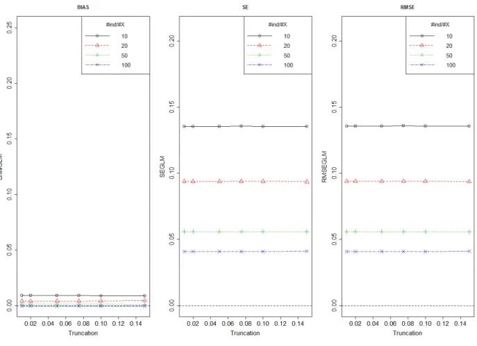
Figure 7: Bias, SE and RMSE of treatment effect estimated by the GLM method using different number
of individuals per covariate and for different level of truncation (approach A)
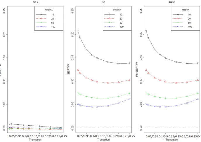
Figure 8: Bias, SE and RMSE of treatment effect estimated by the IPTW method using different number
of individuals per covariate and for different level of truncation (approach B)
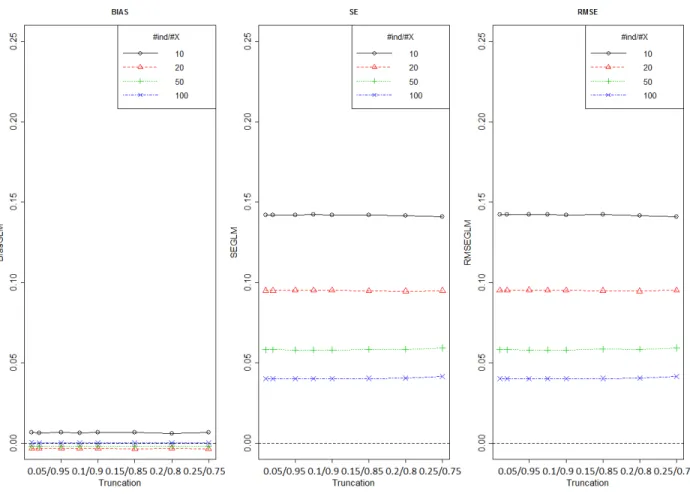
Figure 9: Bias, SE and RMSE of treatment effect estimated by the GLM method using different number
of individuals per covariate and for different level of truncation (approach B)
Figure 10: Density curves of the true underlying probability of receiving treatment and the estimated propensity score ̂ for different degrees of over-fitting
Figure 11: Agreement of the estimated propensity score and true propensity score conditional to
different degrees of over-fitting
Figure 12: Density curves of the true underlying probability of receiving treatment and the estimated propensity score ̂ for different degrees of over-fitting
Figure 13: Agreement of the estimated propensity score and true propensity score conditional to
different degrees of over-fitting
9
List of abbreviations
PS: Propensity Score
hd-PS: High-Dimensional Propensity Score
SPGD: “ o e de P ope sio de G a de Di e sio LDI: Lady Davis Institute for Medical Research EM-algorithm: Expectation maximization algorithm ROC curve: Receiver Operating Characteristics curve AUC: Area Under Curve
SD: Standard Deviation MSE: Mean Squared Error RMSE: Root Mean Square Error GLM: Generalized Linear Model
10
Foreword
This epo t as ealised ithi the f a e o k of Maste de “ iences, Technologies, Santé, Mention Mathé ati ues et Appli atio s “pé ialité “tatisti ue u de the supe isio of D . Ro e t W. Platt and Dr. Tibor Schuster. An abstract on this topic has been selected for an oral presentation at the 34th Annual Conference of the ISCB (International Society for Clinical Biostatistics) on 25 – 29 August 2013 in Munich, Germany. A manuscript will be submitted to a peer-review by the end of August 2013.
11
Host organization presentation
In order to fulfill the requirements of my statistics Master program at Strasbourg University, I did my final internship (stage de fi d’études) at the Department of Epidemiology, Biostatistics and Occupational Health of McGill University. My office was located in the Centre for Clinical Epidemiology of The Lady Davis Institute for Medical Research (LDI). McGill University is located in Montreal, Quebec, Canada and was founded in 1821 by James McGill, a prominent Scottish merchant. Eight years after it as offi iall esta lished, M Gill College ega holdi g lasses i o ju tio ith the Mo t eal Medical Institution.
The LDI is the esea h a of Mo t eal’s Je ish Ge e al Hospital, a tea hi g hospital of M Gill U i e sit . Fou ded i , the LDI is o e of Ca ada’s leadi g health esearch institutes. Important discoveries which have contributed to the health and well-being of patients in Quebec, Canada, and around the world, have been made by LDI researchers in the areas of HIV/AIDS, aging, cancer, vascular disease, epidemiology, and psychosocial science. At the time of my internship, about 200 researchers worked at the LDI. About 20% were primarily lab-based, 15% investigated psychosocial aspects of disease or do research in epidemiology, while the majority were principally involved in clinical research and other types of investigations.
The Centre for Clinical Epidemiology and Community Studies was founded in 1991 by Drs. Lucien Abenhaim and Samuel Orkin Freedman. Under the guidance of Dr. Abenhaim (Director from 1991 to 1999) the centre has established itself as a leader in pharmacoepidemiology, randomized clinical trials, neuroepidemiology, health services research, cardiovascular epidemiology, epidemiology of thromboembolic disorders, geriatrics, and emergency medicine. Dr. Samy Suissa was appointed the Director of the Centre in June 2010.
12
Acknowledgments
I would like to acknowledge the following people for their support and assistance during this internship. First, I would like to thank my immediate supervisor Dr. Robert Platt for giving me the opportunity to do an internship in his team. It was a great experience and an opportunity for me to work in Canada. It also helped me to improve my English and my interest in biostatistics and to have specific plan for my future career.
I also would like to thank my colleague Dr. Tibor Schuster who agreed to serve as one of my internship advisors and for his many contributions to my work, for his patience and for being my brave collaborator during all my internship. I also would like to thank all the people and colleagues who worked in the Centre for Clinical Epidemiology with me for openness they created an enjoyable working environment. I would like to thank Ludovic Trinquart and Raphael Porcher for their advice and their availability.
Furthermore, I would like to thank also my best friend Michelle Liendze, my roommate and my friend Vanessa Nanfah, my brother Guy Kouokam, my aunt Cecile Waffo and all my friends for their attention and encouragement during my stay in Canada. The families I most wish to thank are Guennec family, Lemoine family, Maheu family, De Laval family and Kouokam family for whom my graduate studies in France would not have been possible and who held faith in me and pushed me to succeed!
I would like to thank the Alsace Region for scholarship grant of mobility. Finally I thank all my teachers of the Department of Statistics of the University of Strasbourg for their lessons and advice during my Master. This internship would not have been possible without their lessons.
13
Chapter 1: Introduction
1.1 Context and objectives
The propensity score-based analysis is an advanced method of dealing with confounding in non-randomized studies. Confounding of treatment effect estimates occurs when a factor is associated with the treatment assignment and at the same time is related to outcome. The propensity score for an individual is the probability of receiving the experimental treatment (as compared to the control treatment), conditional on the i di idual’s o a iate alues. The propensity score can be used to balance the covariate distributions between the interesting comparison groups of a study (treated/untreated or exposed/unexposed), and thus reduce bias potentially caused by the considered covariates D’Agosti o 1998).
Popular propensity score approaches are either adjustment for the propensity score in context of multivariable modelling, matching on the propensity score o usi g the i e se of a i di idual’s propensity score as weight within the framework of marginal structural models (Austin and Mamdani 2006). Marginal structural models are a relatively new class of causal models in which the model parameters are estimated through inverse-probability-of-treatment weighting approach. These models allow for appropriate adjustment for confounding (Hernán, Brumback, and Robins 2000).
In literature, over-fitting can occur in application of the propensity score (Cepeda et al. 2003; Stürmer et al. 2005). It occurs in studies where there are too few patients relative to the number of covariates. This is a particular problem when analysing large data bases as for example when using high dimensional propensity score to automate confounding control in distributed medical product safety surveillance systems (Rassen and Schneeweiss 2012). The high dimensional propensity score (hd-PS) is an algorithm that identifies a large number of potential confounders in claims databases, eliminates covariates with very low prevalence and minimal potential for causing bias, and then uses propensity score techniques to adjust for a large number of target covariates (Schneeweiss S. 2009). There are some problems which occur with the hd-PS. Since the algorithm recodes every single count variable into three binary variables, the number of estimated parameters in the propensity score model considerably increases. The choice between selected covariates within the hd-PS in literature varies between 200 and 500 variables (Rassen et al. 2011). However, as shown in previous simulation studies (Peduzzi et al. 1996), the ratio of number of events (treated or untreated) to estimated parameters in the logistic regression model should exceed 10 in order to achieve reliable effect estimates (with acceptable standard errors). These requirements, however, were not satisfied in a number of previously published studies (Rassen et al. 2011; Rassen, Avorn, and Schneeweiss 2010; Cepeda et al. 2003).
Our objective was therefore first to assess the impact of over-fitting of propensity score models when estimating true underlying probabilities to receive treatment and second, how inaccuracies in these estimates translate to erroneous estimates of treatment effects. In particular it was questioned if inaccurate estimation of the propensity score due to over-fitted model leads to considerable bias or inflation of variance in estimating the treatment effect on a typically binary outcome.
14 In chapter 2, we present the propensity score and methods how this score can be used to address confounding in common treatment effect studies. In chapter 3, we describe the design of an extensive Monte-Carlo simulations study to investigate to which extend over-fitting of propensity score models leads to inaccurate estimated propensity scores and their consequences on the estimation of treatment effect estimate. In chapter 4, we describe the results of the effect of over-fitting on correct estimation of the propensity score and performance evaluation of treatment effect estimates.
15
Chapter 2: Propensity score
2.1 Propensity score model
Non-randomized studies on treatment or exposure effects refer to a diverse group of studies that evaluate interventions or exposures which were allocated to individuals by unknown, but certainly non-random, assignment processes. In randomized experiments, the results in the two treatment groups (treated and untreated) may often be directly compared because their units are likely to be similar, whereas in non-randomized experiments, such direct comparisons may be misleading because the units exposed to one treatment generally differ systematically from the units exposed to the other treatment (Rosenbaum 1983). Multivariable analysis is the most commonly used analytic method for dealing with confounding in randomized designs. Other advanced methods of dealing with confounding in non-randomized studies include propensity score analysis and instrumental variable analysis.
The use of propensity scores is a two-stage process: the development of the score model and the use of the score for adjusting for covariate differences. Propensity scores combine a large number of possible confounders into a single variable. In Epidemiology, a confounder refers to a variable that is prognostically linked to the outcome of interest and is unevenly distributed between the study groups: treated/non-treated or exposed/unexposed (figure 1). To calculate the propensity score first one has to identify those variables that influence study group membership (e.g., demographic characteristics, disease severity). The variables that influence group membership are then entered into a logistic model estimating the likelihood of being in a particular group. A logistic model will yield a propensity score for each subject ranging from 0 to 1. The score is the estimated probability of being in one of the both groups (generally it is the treated group), o ditio al o a eighted s o e of that su je t’s alues o the set of variables used to create the score. Rosenbaum and Rubin (Rosenbaum 1983) introduced the propensity score for subject as the conditional probability of assignment to a particular treatment versus control given a vector of observed covariates, :
To understand the strength of propensity scores, one may consider two subjects with identical propensity scores, one who received the intervention and one who did not. If one assumes that the propensity score is based on all those factors that would affect the likelihood of receiving an intervention, then one can consider the assignment of the cases to be essentially random (Rubin 1997). Even if the propensity score is based on all of the factors known to influence group assignment, there remains the possibility that there are unknown confounders. If one could include these unknown confounders, they would change the propensity score. Therefore, two subjects with the same propensity score may not have the same likelihood of being in either group if the propensity score model is misspecified D’Agosti o .
16 Since the propensity score corresponds to a conditional probability, different approaches can be used for estimation. The most commonly used statistical method for estimating the propensity score is binary logistic regression.
2.1.1 Logistic regression model
The logistic regression model is a model in which the response variable is dichotomous and coded 0 and 1. In this model, the expected value is simply the conditional probability that takes the value 1 for an individual with covariate realizations .
This could be modelled as an ordinary linear model:
( )
Here it is assumed that are independent. As the predicted probability must satisfy , the probability is replaced by the logit transformation of the probability, . The observed values of do not follow a normal distribution with mean , but rather a Bernoulli or binomial distribution. The model becomes:
where:
is the th explanatory variable ( );
is the estimated value of the true probability that the variable takes the value 1; is the estimated constant term;
are the estimated logistic regression coefficients.
The logit of the probability is simply the log of the odds of the event of interest. In a logistic regression model, the parameter associated with explanatory variable is commonly interpreted after transforming to , whichis the relative change of the odds that when increases by , conditional on the other explanatory variables remaining the same. Therefore, refers to the odds ratio.
For subject , the estimated propensity score is given by:
̂ ̂ ̂ ̂ ̂ ̂
where ̂ ̂ are the estimated of the regression coefficients. When there are missing values in covariates, one can use the EM algorithm to estimate propensity scores.
17 2.1.2 The EM-algorithm
The EM (Expectation-Maximization) -algorithm is an alternative procedure for computing the maximum likelihood estimator when only a subset of the data is available. The first proper theoretical study of the algorithm was done by Dempster, Laird, and Rubin (A.P. Dempster N.M Laird 1977).
Let be a sample with conditional density given . The log-likelihood function is given by . It is assumed that the data consists of observed variables and unobserved (missing or latent variables) so that . With
this notion the log-likelihood function for the observed data is ∫ . The problem here is that when maximizing the likelihood a complete integral is required. One might not be able to find a closed form expression for . To maximize with respect to the idea is to do an iterative procedure where each iteration has two steps, called the -step and the -step. Let
denote the estimate of after the th step. Then the two steps in the ( +1)th iteration are:
-step: Compute ( | ) .
-step: Maximize ( | ) with respect to and put argmax . This procedure is
iterated until it converges. Given the description just showed above, a reasonable convergence test would be to check if the increase of between successive iterations is smaller than some tolerance parameter, and to declare convergence if the EM-algorithm is not considerably improving anymore.
Generally, the EM-algorithm works best when the fraction of missing information is small and the dimensionality of the data is not too large.
2.1.3 Variables in the propensity score
Once the propensity score is created, it can be used to adjust for covariate differences in four different ways: matching, stratification, as a covariate in a multivariable analysis, and as a method for weighting observations Rose au ; Ru i ; D’Agosti o . Two important questions arise with regard to how to calculate propensity scores: what variables to include in a propensity score and how to assess the adequacy of propensity scores.
It might seem sufficient to include only those variables that are associated with both the treatment and the outcome. After all, if a variable is not a confounder then its inclusion in the propensity score is not likely to improve the adjustment for differences between the two groups (Katz 2010). Missing a confounder is a much more relevant problem than including a variable that is associated with group membership but is not with the outcome.
18
Figure 1: Graph representing confounding variables.
In figure 1, boxes represent variables and arrows represent directed effects. If one can remove the confounder to the treatment arrow, one can remove the effect of confounding. Patients with equivalent probabilities of treatment will not induce a confounder to treatment association.
2.1.4 Adequacy of the propensity score: the ROC curve
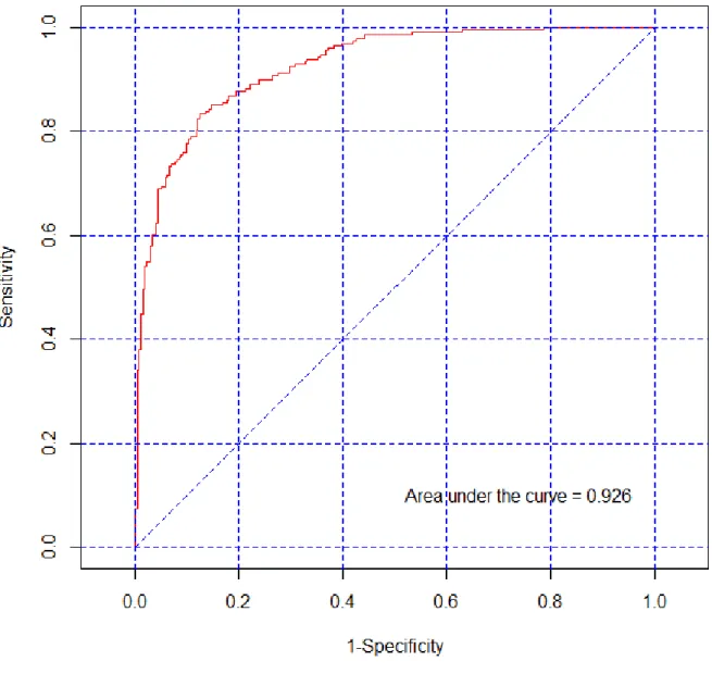
Once propensity score is calculated using those variables that differ between the groups, one desired property of the score is the ability of the propensity score to differentiate those who received the intervention from those who did not. To assess how well the propensity score differentiates those who receive the intervention from those who do not, one can use the area under the receiver operating characteristics (ROC) curve AUC (Petrie and Sabin 2009), which is also referred as the concordance index (c-index) (Katz 2006). An AUC value of 0.5 indicates that the model does not distinguish any better than chance. The maximum is one. The higher the c-index, the better the model is at distinguishing the two groups. A ROC curve can be constructed by plotting the sensitivity of the propensity score (in predicting who received the intervention) on the -axis (true positive rate) and (1-specificity) on the -axis (false positive rate).
Figure 2 shows an example of a single ROC curve from a propensity score model. In this model one have a sample with 500 individuals. There are 100 predictors and no interactions and the area under the curve represents the probability that a randomly selected treated individual will have a higher propensity score than a randomly selected untreated individual. If the propensity score was perfect, the minimum propensity score of the treated would be higher than the maximum propensity score of the untreated. If the test was worthless, giving no better prediction than a random classification, one would expect that half of the treated would have a higher propensity score value than half of the untreated (and vice versa), as indicated by an AUC value of 0.5.
Confounders
Outcome Treatment
19
Figure 2: An example of a ROC curve.
2.2 Propensity score confounder adjustment methods
20 2.2.1 Matching using propensity score
The concept of propensity score matching was first introduced by Rosenbaum and Rubin (Rosenbaum 1983). Propensity score matching refers to the pairing of treatment and controls units with similar values on the propensity score, and possibly other covariates, and the discarding of all unmatched units (Rubin 2001). It is primarily used to compare two groups of subjects but can be applied to analyses of more than two groups. The most common implementation of propensity score matching is pair matching or 1:1 matching in which matched pairs of treated and untreated subjects are formed (Austin 2012). The major advantage of matching on propensity scores is that compared to other propensity score methods it generally provides the least biased estimates of treatment effect (Austin 2007). A disadvantage of matching by propensity score is that the matched sample may be smaller and not representative of the study population, thereby decreasing generalizability of results.
2.2.2 Stratifying by propensity score
Since it is not always possible to find (near) exact matches on propensity score between cases and controls, one may instead stratify cases and controls by propensity scores. This technique consists of grouping subjects into strata determined by similar propensity score. Once the strata are defined, treated and non-treated subjects who are in the same stratum are compared directly. Cochran notes that as the number of covariates increases, the number of strata grows exponentially (Cochran 1965). For instance, if all covariates were dichotomous categorical variables, then there would be subclasses for covariates. In terms of how many strata to create, five strata have been shown to eliminate about of the bias in unadjusted analyses (Rubin 1997). An analysis comparing five strata to three or equal-sized strata found similar results (Landrum M.B. 2001). A weakness of stratification is that you may have residual confounding. In other words, within each stratum of propensity score there may be important differences on baseline characteristics.
2.2.3 Covariate adjustment using propensity score
Rather than using the propensity score to match cases or to create strata the score can be entered as an independent variable in a multivariable model. In other words, the propensity score would be an independent variable for which the value fo ea h su je t ould e that su je t’s p ope sit s o e. Rosenbaum and Rubin proposed covariate adjustment using the propensity score in the context of estimating linear treatment effects for continuous data (Rosenbaum 1983). In our study, we used this approach to estimate the regression coefficient associated with the treatment.
2.2.4 Inverse probability of treatment weighting (IPTW)
Another way to adjust for baseline differences is to use propensity score to weight the multivariable analysis. This strategy uses the propensity score to assign individual weights to all observations resulting in an altered composition of the study population (Robins, Hernán, and Brumback 2000). The weight of a person receiving the intervention is the inverse of the propensity score; the weight for the control is the
21 inverse of one minus the propensity score. Let denote the treatment assignment ( denoting treatment, denoting no treatment). For a given propensity score the weights are defined to be . For each subject, it is equal to the inverse of the probability of receiving the treatment that the subject received. Some analysts have found that using propensity scores to weight observations is less subject to misspecification of the regression models used to predict average causal effect than using propensity-based stratification (Lunceford and Davidian 2004). A problem with weighting observations is that when the estimated propensity score is near zero or one, the weights may be extreme and unrealistic (Rubin D.N 2001).
22
Chapter 3: Methods
Within the internship project, extensive Monte Carlo simulation studies were conducted to investigate the impact of over-fitting on different criteria i.e. accuracy in estimation of latent treatment allocation probabilities and impact on estimation of treatment effects. The criteria on which the performance is evaluated were bias, standard error (SE) and root mean squared error (RMSE) of the respective estimator.
All analyses were performed by using software ( version 2.15.2 (2012-10-26), R Core Team (2012). R: A language and environment for statistical computing. R Foundation for Statistical Computing, Vienna, Austria. ISBN 3-900051-07-0, URL http://www.R-project.org/.)
3.1 Effect of over-fitting on correct estimation of the propensity score
The data simulation was conducted as follows: A total of 100 baseline covariates were generated assuming to be independently normally distributed with mean 0. The variance of the normal distributed covariates was specified in a way, that extreme propensity score values (below 0.05 or above 0.95), would not exceed a prevalence of 5%. To accomplish this, the corresponding regression coefficients were sampled from a beta distribution with the two shape parameters a=0.5 and b=2. The sign of each regression coefficient was assigned by random sampling from a Bernoulli distribution with parameter p=0.5.This configuration was chosen in order to facilitate simulation of realistic treatment prediction scenarios which do not reveal too many strong predictor variables potentially leading to extreme propensity score values close to 0 or 1.
A logistic regression model was used to specify the true probability of receiving treatment for the simulated values of the linear predictor:
The intercept was chosen to be in order to achieve stochastically balanced numbers of exposed and unexposed individuals in the simulation. For each individual, the exposure status was sampled from a Binomial distribution with parameter . In order to initiate different magnitudes of over-fitted propensity score models, the number of individuals per covariate were set to and . Within each of these datasets, the sample-specific propensity score ̂ was estimated via logistic regression on the binary outcome including all 100 covariates. This procedure, data simulation, sampling and propensity score estimation, was repeated 1000 times for each of the five sample size scenarios.
23
3.2 Over-fitting and related bias, variance and MSE of treatment effect
estimates
In order to evaluate the effect of over-fitting on bias and variance of treatment effect estimates, we considered the common case of a binary outcome variable . The effect of treatment on was specified by different log odds ratio values . The outcome variable was sampled from a binomial distribution with parameter derived based on another logistic regression model containing the simulated covariates and the previously generated exposure variable:
Likewise the treatment predicting effects, the regression coefficients were sampled from a beta distribution with the two shape parameters a=0.5 and b=2. The sign of each regression coefficient was again assigned by random sampling from a Bernoulli distribution with parameter p=0.5. Here again, the intercept was chosen to be 0 leading to an expected outcome prevalence of 0.5. By choosing this simulation setting we assured that predictor variables represent real confounders i.e. being associated with both the treatment and the outcome.
To estimate the interesting treatment effect , three approaches were considered: A) multivariable logistic regression model (GLM) considering deciles of the estimated propensity score as adjustment variable next to the treatment variable (we used propensity score deciles because it is recommended in literature (Rassen et al. 2011)), B) weighted logistic regression model for the estimation of the marginal exposure effect using the estimated propensity score to generate individual weights
̂
̂
(inverse probability of treatment weighting: IPTW) and C) matching on the estimated propensity score. In the case of multivariable logistic regression model, the dependent variable was the outcome, and the independent variables were the exposure variable and the propensity score recoded into deciles. For the weighted logistic regression model, the dependent variable was the outcome and the independent variable was the exposure. In the case of matching, one used a greedy-matching algorithm to match subjects using caliper that were defined to have a maximum width of 0.2 standard deviations of the estimated propensity score. The caliper wide was chosen according to recommendations in literature (Austin and Mamdani 2006). For each generated data sample in the simulation, the above two logistic regression models (GLM and IPTW) were fitted, matching was applied and the resulting effect estimate ̂ were retrieved. The bias, defined as the expected value of the difference between the effect estimate ̂ and the true effect , was calculated by taking the mean of this difference over all 1000 simulations runs. The empirical standard error of the estimator was calculated by calculating the standard deviation of ̂ over all 1000 simulations runs. To evaluate the precision of effect estimates, we estimated the standard error using the square root of the sample variance of the treatment effect estimates across all 1000 simulation runs. The root mean square error (RMSE) was calculated by taking the square root of the mean of the squared errors over all the simulation runs. It was calculated to summarize estimation performance.
24
3.3 Truncation
As we use propensity score to define individual weights within a weighted multivariable analysis, extreme weights may be generated when propensity score is near zero or one. To overcome the issue of instable weights, we followed to approaches:
A) Elimination of extreme values of the estimated propensity score by quantile truncation of the tails of the observed propensity score distribution.
B) Elimination of extreme values of the estimated propensity score by restricting the scale of the propensity score to less extreme values than 0 or 1. All observed propensity score values which exceed the respective restriction criteria, were truncated.
In general, it is expected that a higher truncation level leads to a decrease in variance of the estimator but on the other hand to an increment of bias. Therefore, in order to find the best threshold for truncation which minimizes the MSE of the IPTW estimator, six levels of truncation were considered when applying truncation approach A): , , and
For truncation approach B) the following min/max values for the propensity score were considered as truncation boundaries: , , , , , , and .
25
Chapter 4: Results
4.1 Effect of over-fitting on correct estimation of the propensity score
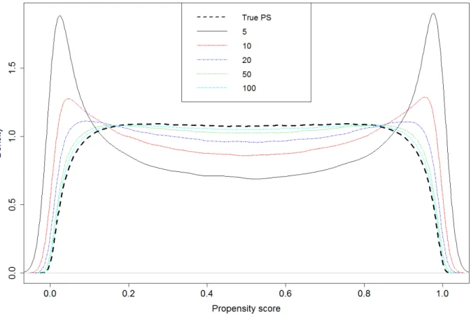
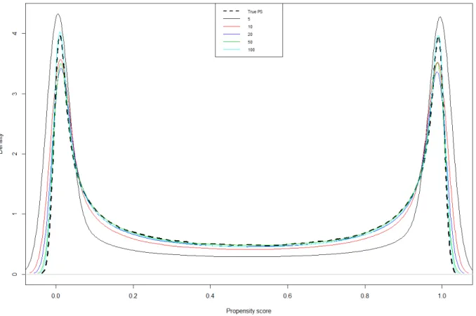
Figures 3 and 4 represent the effect of over-fitting on correct estimation of the propensity score. They show how estimation of propensity score is influenced by over-fitting. Figure 3 represents the density curves of the true underlying probability of receiving treatment and the estimated propensity score ̂ for different degrees of over-fitting. As can be seen from the figure 3, if the number of individuals
per covariate is low (<=20, corresponding to a number of treated <=10), the density curve of the estimated propensity score deviates considerably from the curve of the true underlying probability of receiving treatment. In particular, when the number of individuals per covariate equals 5, there were many individuals who got assigned a propensity score close to 0 or 1.
Figure 3: Density curves of the true underlying probability of receiving treatment and the estimated propensity score ̂ for different degrees of over-fitting.
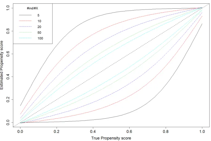
26 Figure 4 shows the agreement of estimated propensity score and true propensity score conditional to different degrees of over-fitting.
Figure 4: Agreement of the estimated propensity score and true propensity score conditional to different degrees of over-fitting.
Figure 4 displays for each number of individuals per covariate (degree of over-fitting) and for a given value of the true propensity score the 95% distribution interval of the respectively estimated propensity scores. These intervals were obtained by the 0.025 and 0.975 quantiles of the distribution of estimated propensity scores over all 1000 simulation runs. When the number of individuals per covariate in the propensity score is low (<=20, number of treated <=10), the 95% distribution intervals are large. The dashed black diagonal line represents the ideal value (perfect agreement) of the estimated propensity score for a given value of the true propensity score.
27
4.2 Over-fitting and related bias, variance and MSE of treatment effect
estimates
Figure 5 represents the effect of over-fitting on a parameter estimation. It shows bias, root mean squared error and standard error in estimating the treatment effect for each number of individuals per covariate resulting from both IPTW and ordinary multivariable adjustment approaches and from matching. The black dots represent the estimate of the treatment effect by the IPTW method, the triangles are for the GLM approach and the stars are for matching.
One can see that the bias is
negligible whatever the degree of over-fitting. On the other hand, when the number of
individuals per covariate is low (<=20,
number of treated<= 10) the SE increases considerably. As
the bias is close to 0, the RMSE and the SE have approximately the same values.
Figure 5: Bias, SE and RMSE of treatment effect estimated by both GLM and IPTW methods and by matching, for .
4.3 Truncation
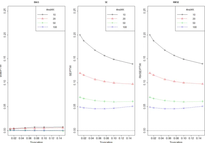
Figure 6 shows bias, SE and RMSE of treatment effect estimated by IPTW method using different number of individuals per covariate and for different level of truncation boundaries (truncation approach A). This figure is drawn only for One can see that the bias is negligible so the SE and the RMSE have the same value. The dataset which correspond to the number of individuals per
28 covariate 5, was excluded because the model did not converge. As expected, with increasing number of individuals per covariate, the standard error of the estimator decreased.
Figure 6: Bias, SE and RMSE of treatment effect estimated by IPTW method using different number of individuals per covariate and for different level of truncation (approach A)
Figure 7 shows bias, SE and RMSE of treatment effect estimated by GLM method using different number of individuals per covariate and for different level of truncation (truncation approach A). This figure is drawn only for One can see that the bias is negligible so the SE and the RMSE have the same value. Here again, the dataset which correspond to the number of individuals per covariate 5, was excluded because the model did not converge. The bias, the SE and the RMSE of the treatment effect estimated by the GLM approach are constant whatever the level of truncation.
29
Figure 7: Bias, SE and RMSE of treatment effect estimated by GLM method using different number of individuals per covariate and for different level of truncation (approach A)
Figure 8 shows bias, SE and RMSE of treatment effect estimated by IPTW method using different number of individuals per covariate and for different level of truncation boundaries (truncation approach B). This figure is drawn only for One can see that the bias is negligible so the SE and the RMSE have the same value. The dataset which correspond to the number of individuals per covariate 5, was excluded because the model did not converge. As expected, with increasing number of individuals per covariate, the standard error of the estimator decreased. The MSE curves show an approximately quadratic shape with increasing level of truncation. The minimum MSE occurred for truncation levels between 0.05 and 0.10 suggesting the best possible stabilisation of weights by truncation.
30
Figure 8: Bias, SE and RMSE of treatment effect estimated by IPTW method using different number of individuals per covariate and for different level of truncation (approach B)
Figure 9 shows bias, SE and RMSE of treatment effect estimated by GLM method using different number of individuals per covariate and for different level of truncation (truncation approach B). This figure is drawn only for One can see that the bias is negligible so the SE and the RMSE have the same value. Here again, the dataset which correspond to the number of individuals per covariate 5, was excluded because the model did not converge. The bias, the SE and the RMSE of the treatment effect estimated by the GLM approach are constant whatever the level of truncation.
31
Figure 9: Bias, SD and RMSE of treatment effect estimated by GLM method using different number of individuals per covariate and for different level of truncation (approach B)
32
Chapter 5: Discussion
5.1 Key results and Limitations
We conducted an extensive series of Monte Carlo simulations first, to assess the impact of over-fitting of propensity score models when estimating true underlying probabilities to receive treatment and second, to see how inaccuracies in these estimates translate to erroneous estimates of treatment effects. There is considerable imprecision in estimation of the propensity score if the ratio between the number of individuals and the number of covariates in the propensity score is low (<=20, number of treated individuals per covariate <=10).
There are certain limitations to our study. First, our findings were based on simulations which can never capture the whole space of possible data scenarios as they occur in reality. However, since we were mainly interested in the statistical properties of different estimators for the propensity score and treatment impact on an outcome, real data application would have been not useful due to a lack of knowledge of the respective true underlying effects. In our study we only investigated truncation as one possibility to address unstable weights as induced by extreme propensity score values. An other possible option would have been the utilization of stabilized weights. For this purpose the numerator of the weights can be modified, which decreases variability (Robins, Hernán, and Brumback 2000). Stabilized weights might reduce the estimation problem induced by over-fitted propensity score models. In our study, the number of covariate is fixed and the number of individuals varies and it has a direct influence on the RMSE. It would be a good idea to fix the number of individuals and to vary the number of covariates.
5.2 Conclusion and perspectives
The simulations demonstrate the problems that can occur when the propensity score model contains few individuals relative to the number of independent variables being evaluated. They revealed that over-fitting of propensity scores should be avoided in order to facilitate reliable estimates of treatment effects. While methods exist to address this, e.g., truncation or stabilization, researchers should be cautious when the number of predictors is high relative to the number of treated or untreated individuals in the propensity score model. According to our study, we can suggest that at least 25 treated or untreated individuals per covariate in the propensity score model are desirable to maintain valid propensity score estimates and to avoid overly inflated standard errors of treatment effect estimates.
33
References
A.P. De pste N.M Lai d. . Ma i u Likelihood f o I o plete Data ia the EM Algo ith .
Journal of the Royal Statistical Society 39. B.
Austi , Pete C. . The Pe fo a e of Diffe e t P ope sit “ o e Methods fo Esti ati g Ma gi al Odds Ratios. Statistics in Medicine 26 (16) (July 20): 3078–3094. doi:10.1002/sim.2781.
———. . The Pe fo a e of Diffe e t P ope sit “ o e Methods for Estimating Marginal Hazard Ratios. Statistics in Medicine (December 12). doi:10.1002/sim.5705.
Austi , Pete C, a d Muha ad M Ma da i. . A Co pa iso of P ope sit “ o e Methods: a Case-study Estimating the Effectiveness of post-AMI Statin Use. Statistics in Medicine 25 (12) (June 30): 2084–2106. doi:10.1002/sim.2328.
Cepeda, M “oledad, Ra Bosto , Joh T Fa a , a d B ia L “t o . . Co pa iso of Logisti Regression Versus Propensity Score When the Number of Events Is Low and There Are Multiple Co fou de s. American Journal of Epidemiology 158 (3) (August 1): 280–287.
Co h a . . The Pla i g of O se atio al “tudies of Hu a Populatio s.
D’Agosti o, R B, J . . P ope sit “ o e Methods fo Bias Redu tio i the Co pa iso of a Treatment to a Non-a do ized Co t ol G oup. Statistics in Medicine 17 (19) (October 15): 2265–2281.
He á , M A, B B u a k, a d J M Ro i s. . Ma gi al “t u tu al Models to Esti ate the Causal Effect of Zidovudine on the Survival of HIV-positive Men. Epidemiology (Cambridge, Mass.) 11 (5) (September): 561–570.
Katz, Mitchell H. 2006. Multivariable Analysis: a Practical Guide for Clinicians. d ed. Ca idge ; Ne York: Cambridge University Press.
———. 2010. Evaluating Clinical and Public Health Interventions: a Practical Guide to Study Design and
Statistics. Ca idge: Ne Yo k : Ca idge U i e sit P ess.
La d u M.B. . Causal Effe t of A ulato “pe ialt Ca e o Mo talit Follo i g M o a dial Infarction: A Comparison of Propensity and Instru e tal Va ia le A al ses.
Lu efo d, Ja ed K, a d Ma ie Da idia . . “t atifi atio a d Weighti g ia the P ope sit “ o e i Esti atio of Causal T eat e t Effe ts: a Co pa ati e “tud . Statistics in Medicine 23 (19) (October 15): 2937–2960. doi:10.1002/sim.1903.
Peduzzi, P, J Co ato, E Ke pe , T R Holfo d, a d A R Fei stei . . A “i ulatio “tud of the Nu e of E e ts Pe Va ia le i Logisti Reg essio A al sis. Journal of Clinical Epidemiology 49 (12) (December): 1373–1379.
Petrie, Aviva, and Caroline Sabin. 2009. Medical Statistics at a Glance. Chichester, UK; Hoboken, NJ: Wiley-Blackwell.
Rasse , Je e A, Je A o , a d “e astia “ h ee eiss. . Multi a iate-adjusted
Pharmacoepidemiologic Analyses of Confidential Information Pooled from Multiple Health Care Utilizatio Data ases. Pharmacoepidemiology and Drug Safety 19 (8) (August): 848–857. doi:10.1002/pds.1867.
Rasse , Je e A, Ro e t J Gl , M Ala B ookha t, a d “e astia “ h ee eiss. . Co a iate Selection in High-di e sio al P ope sit “ o e A al ses of T eat e t Effe ts i “ all “a ples.
34 Rasse , Je e A, a d “e astia “ h ee eiss. . Usi g High-dimensional Propensity Scores to
Auto ate Co fou di g Co t ol i a Dist i uted Medi al P odu t “afet “u eilla e “ ste .
Pharmacoepidemiology and Drug Safety 21 Suppl 1 (January): 41–49. doi:10.1002/pds.2328.
Ro i s, J M, M A He á , a d B B u a k. . Ma gi al “t u tu al Models a d Causal I fe e e i Epide iolog . Epidemiology (Cambridge, Mass.) 11 (5) (September): 550–560.
Rose au , Ru i . . The Ce t al Role of the Propensity Score in Observational Studies for Causal Effe ts. Biometrika 70 (April).
Ru i , D B. . Esti ati g Causal Effe ts f o La ge Data “ets Usi g P ope sit “ o es. Annals of
Internal Medicine 127 (8 Pt 2) (October 15): 757–763.
Rubi D.N. . Usi g P ope sit “ o es to Help Desig O se atio al “tudies: Appli atio to the To a o Litigatio .
“ h ee eiss “. . High-dimensional Propensity Score Adjustment in Studies of Treatment Effetcs Usi g Health Ca e Clai s Data.
Stürmer, Til, Sebastian Schneeweiss, M Alan Brookhart, Kenneth J Rothman, Jerry Avorn, and Robert J Gl . . A al ti “t ategies to Adjust Co fou di g Usi g E posu e P ope sit “ o es a d Disease Risk Scores: Nonsteroidal Antiinflammatory Drugs and Short-term Mortality in the Elde l . American Journal of Epidemiology 161 (9) (May 1): 891–898. doi:10.1093/aje/kwi106.
35
Annexes
Annexe 1: Simulations when the regression coefficients were on the joined
interval
]
We simulated data for a setting in which there were 100 baseline covariates which were independently standard normal distributed. In order to initiate real confounding situations, the regression coefficients were sampled from a uniform distribution on the joined interval . We allowed covariates to have a strong effect of treatment selection or outcome. Confounding effects are small if the regression coefficients are close to . We use a logistic regression model to specify the true probability of receiving treatment for the simulated values of the linear predictor:
The intercept was chosen to be in order to achieve stochastically balanced numbers of exposed and unexposed individuals in the simulation. The prevalence will be 50 percent because has expectation to be . For each individual, the exposure status was sampled from a Binomial distribution with parameter . is a function of the (when we estimate the propensity score with a logistic regression, the outcome variable is the exposure ). In order to initiate different magnitudes of over-fitted propensity score models, the number of individuals per covariate were set to and . Within each of these datasets, the sample-specific propensity score ̂ was estimated via logistic
regression on the binary outcome including all 100 covariates. This procedure, data simulation, sampling and propensity score estimation, was repeated 1000 times for each of the five sample size scenarios.
Annexe 2: Results when the regression coefficients were on the joined interval
Figure 10 shows the density curves of the true propensity score and estimated propensity score for different degrees of over-fitting. As one can see that when the number of individuals per covariate is low (<=20), the density curve of the estimated propensity score deviates from the density curve of the true propensity score.
36
Figure 10: Density curves of the true underlying probability of receiving treatment and the estimated propensity score
̂ for different degrees of over-fitting.
We can see that for each density curve even for the true propensity score, there are many individuals who have extreme propensity score values close to 0 or 1. This scenario is not good for our study because later, we use propensity score to weight a multivariable analysis in order to estimate the effect of treatment. And in this case, many unrealistically extreme weights would be generated. That is why we have decided to sample the regression coefficients from a beta distribution with the two shape parameters a=0.5 and b=2.
37
Figure 11: Agreement of the estimated propensity score and true propensity score conditional to different degrees of over-fitting.
One can see that for each number of individuals per covariate and for a given value of the true propensity score, one have the 95% distribution interval in which should fit the corresponding values of the estimated propensity score. These intervals are non-parametric and they were obtained by the quantiles of the propensity score. When the number of individuals per covariate in the propensity score is low (<=20), the gap between the two lines of the confidence interval is large. The dash line at the center of the graph represents the perfect value of the estimated propensity score for a given value of the true propensity score.
Annexe 3: Simulations when the regression coefficients were on the joined
interval
We simulated data for a setting in which there were 100 baseline covariates which were independently standard normal distributed. In order to initiate real confounding situations, the regression coefficients were sampled from a uniform distribution on the joined interval . We allowed covariates to have a weak effect of treatment selection or outcome. As the regression coefficients are close to , confounding effects are small. We use a
38 logistic regression model to specify the true probability of receiving treatment for the simulated values of the linear predictor:
The intercept was chosen to be in order to achieve stochastically balanced numbers of exposed and unexposed individuals in the simulation. The prevalence will be 50 percent because has expectation to be . For each individual, the exposure status was sampled from a Binomial distribution with parameter . is a function of the (when we estimate the propensity score with a logistic regression, the outcome variable is the exposure ). In order to initiate different magnitudes of over-fitted propensity score models, the number of individuals per covariate were set to and . Within each of these datasets, the sample-specific propensity score ̂ was estimated via logistic
regression on the binary outcome including all 100 covariates. This procedure, data simulation, sampling and propensity score estimation, was repeated 1000 times for each of the five sample size scenarios.
Annexe 4: Results when the regression coefficients were on the joined interval
Figure 12 shows the density curves of the true propensity score and estimated propensity score for different degrees of over-fitting. As one can see that when the number of individuals per covariate is low (<=20), the density curve of the estimated propensity score deviates considerably from the density curve of the true propensity score.
39
Figure 12: Density curves of the true underlying probability of receiving treatment and the estimated propensity score
̂ for different degrees of over-fitting.
One can see that for each density curve even for the true propensity score, there are many individuals who have propensity score values between 0.3 and 0.7. In this case, covariates have a weak effect of treatment selection or outcome. This situation is not realistic. That is the second raison why we have decided to sample the regression coefficients from a beta distribution with the two shape parameters a=0.5 and b=2.
40
Figure 13: Agreement of the estimated propensity score and true propensity score conditional to different degrees of over-fitting.
One can see that for each number of individuals per covariate and for a given value of the true propensity score, one have the 95% distribution interval in which should fit the corresponding values of the estimated propensity score. These intervals are non-parametric and they were obtained by the quantiles of the propensity score. When the number of individuals per covariate in the propensity score is low (<=20), the gap between the two lines of the confidence interval is large. The dash line at the center of the graph represents the perfect value of the estimated propensity score for a given value of the true propensity score.