A Statistically adaptive sampling policy to the Hotelling's T2 Control Chart: Markov Chain Approach
Asghar Seifa, Alireza Farazb, Cédric Heuchennec and Erwin Sanigad
aDepartment of Statistics, Islamic Azad University, Hamadan Branch, Hamadan, Iran; bHEC Management School of the University of Liège;
cHEC Management School of the University of Liège and Institute of Statistics, Biostatistics and Actuarial Sciences, Université catholique de Louvain, Belgium;
dBusiness Administration, University of Delaware, Newark, DE 19716, USA
Abstract
This paper proposes an alternative sampling scheme to the Hotelling’s T2 control chart with variable parameters (VP T2). Indeed, the sampling interval h, the sample size n and the control limit k vary between minimum and maximum values while the warning line is kept fixed over time. The proposed method uses only one measurement scale and therefore overcomes the usual difficulties of using two scales. Finally, we show the merits of the proposed method as a good option for its ease of application and its quick responses to small and moderate shifts in a multivariate process.
Keywords: Multivariate Control Chart, Hotelling’s T2 Control Chart, Variable Parameters (VP), Genetic Algorithm (GA), Adjusted Average Time to Signal (AATS).
1. Introduction
Quality control problems in industry may involve more than a single quality characteristic, i.e., a vector of characteristics. The Hotelling’s (1947) T2 control chart is one of the most widely used tools in multivariate statistical process control. Consider a process in which p correlated characteristics are being measured simultaneously and controlled jointly. It is assumed that the joint probability distribution of the quality characteristics is a p-variate normal distribution with the vector of in-control means µʹ′0 =(µ01,...,µ0p) and the variance-covariance matrix∑.
The procedure requires computing the sample means for each of the p quality characteristics from a sample of size n. The vector xʹ′=(x1,...,xp) gives the p sample
bResearch supported by IAP research network P7/06 of the Belgian Government (Belgian Science Policy).
cResearch supported by IAP research network P7/06 of the Belgian Government (Belgian Science Policy), and by the contract
`Projet d'Actions de Recherche Concertées' (ARC) 11/16-039 of the `Communauté française de Belgique', granted by the `Académie universitaire Louvain'.
means. Then the subgroup statistics T2 =n(x−µ0)ʹ′∑−1(x−µ0)are plotted on a control chart in sequential order. For the sake of simplicity, we assume here that µ 0 and ∑ are known or are estimated from large enough samples. In this case, T2 is distributed as a chi square random variable with p degrees of freedom. Each of the T2 values is compared with the upper α percentage of the chi square distribution ( k = 2( ,p)
α
χ ) and if the sample values fall below the control limit k the process is considered in control, otherwise the process is said to be out of control and the corresponding subgroup(s) investigated. It is usually assumed that the variance-covariance structure of the quality characteristics being charted does not change and that assignable causes are manifested by a shift at least in one component of the mean vector of the process. The magnitude of this shift is often expressed
by (µ µ ) 1(µ µ0)
0 ʹ′∑ − −
= 1 − 1
2
d , the Mahalanobis distance, and µ is the out of 1 control mean vector. In this case, the T2 statistic is distributed as a non-central chi-square distribution with p degrees of freedom and non-centrality parameter nd2
= η (Faraz and Parsian, 2006).
The traditional practice in applying the T2 chart is to obtain samples of fixed size n0 at constant intervals h0 which is called a Fixed Ratio Sampling (FRS)
scheme, but it is slow in detecting a small to moderate process shifts. Recently, the ideas of the variable sample sizes (VSS) (see, Faraz and Moghadam, 2009; Faraz et al. 2010), double sampling scheme (DS) (see, Faraz et al. 2012a; Tornga and Lee, 2009), variable sampling intervals (VSI) (see, Amin and Hemasinha, 1993; Chengular et al. 1989; Faraz et al., 2011); variable sample sizes and sampling intervals (VSSI) (see, Costa 1998; Faraz et al. 2012b), double warning lines scheme (DWL) (see, Faraz and Parsian, 2006; Faraz and Saniga, 2011), variable sample sizes and control limits (VSSCL) (see, Chen and Hsieh, 2007; Seif et al. 2011 a&b), variable sampling intervals and control limits (VSICL) (see, Torabian et al. 2010) and variable parameters VP (see, Costa 1999; Chen, 2007; Lin, 2009; Faraz et al. 2013 a&b) has been proposed in literature to provide users with a tool that detects small shifts more quickly than the classical FRS scheme. The question arises that which scheme is the most effective and powerful. Faraz and Parsian (2006) through a comparison between the FRS, VSS, VSI, VSSI and DWL schemes (the VP and
VSSCL are not included) have shown that the DWL scheme is more powerful than the other schemes in detecting small, moderate and even large shifts. Chen (2007)
extended the VP scheme proposed by Costa (1999) to multivariate case and compared the two-scaled variable parameter (2VP) T2 chart with the VSS, VSI, and VSSI T2 charts (the DWL scheme is not included) and the results indicate that the 2VP T2 chart outperforms the VSS, VSI, and VSSI T2 charts, especially in detecting small shifts. However, the 2VP scheme is dominated by the VSI scheme when the process change in the mean vector is moderate or large. The same result is obtained by Chen and Hsieh (2007) and they showed that the two-scaled variable sample sizes and control limits (2VSSC) T2 chart presents a similar performance to the 2VP T2 chart. The proposed 2VP and 2VSSC schemes require the user to construct a T2 chart with two different measuring scales. One on left hand side and the other on the right hand side. This approach is a tedious and of course unwilling for the practitioners. Hence, in this paper we propose the VP, VSSCL and VSICL T2 control charts in a way that they gains from a single measuring scale, a problem heretofore not addressed. Furthermore, through a comparison between all existing T2
charts using variable ratio sampling schemes, the adaptive sampling policy to the T2 chart is proposed. The paper is organized as follows: in the next section, the Markov chain approach to construct VP, VSSCL and VSICL T2 charts are discussed. The performance measure and GA approach to statistically optimal design of the schemes are then studied afterwards. The section 3 makes a comparison between the VP, VSSCL, VSICL, DWL, VSSI, VSS and VSI schemes and finally the optimal sampling policy is then proposed.
2. The VP, VSSCL and VSICL T2 Schemes: Markov Chain Approach
The VP T2 control chart is an extension of the VSSI T2 control chart discussed
by Faraz and Parsian (2006). Let h and 1 h be maximum and minimum sampling 2 intervals, k and 1 k be maximum and minimum control limits, and n2 1 and n2 be
maximum and minimum sample size respectively, such that0<h <2 h1, 0<k <2 k1
and n1 < n2. Here we refer to the set (k1, h1, n1) as minimum sampling plan and the
set (k2, h2, n2) as maximum sampling plan. The decision to switch between
point on the control chart. If the prior sample point (i-1) falls in the safe region, we use the minimum sampling plan and if the prior sample point (i-1) falls in the warning region, we use the maximum sampling plan for the current sample. Finally, if a sample point falls in the action region, then the process is considered out of control. Here the safe, warning and action regions are given by the warning limit w and the control limit kj. The safe region is given by [0,w), the warning region is given by [w, kj), and the action region is given by [kj, ∞ ) , where j=1 if the prior sample point comes from the minimum plan and j =2 if the prior sample point comes from the maximum plan (see figure 1). The following function summarizes the control scheme of the VP T2 control chart:
(h ,i k ) = i ⎪⎩ ⎪ ⎨ ⎧ < ≤ < ≤ k T w if ) , , ( w T 0 if ) , , ( 1 -i 2 1 -i 2 2 2 2 1 -i 1 1 1 n h k n h k (1) 2.1 Performance Measure
The average time from the process mean shifts until the chart produces a signal is used to measure its statistical efficiency. This statistical measure is called AATS and determines the speed with which a control chart detects a process mean shift. The average time of the cycle (ATC) is the average time from the start of the production until the first signal after the process shift. If the assignable cause occurs according to an exponential distribution with parameter λ then the expected time interval that the process remains in control is 1/λ. Therefore,
λ 1 − = ATC AATS (2)
The memoryless property of the exponential distribution allows the computation of the ATC using the Markov chain approach. The Markov chain approach we employ here is similar to that originally proposed by Faraz and Saniga (2009) in which they made a unification and some corrections to Markov chain approaches to develop control charts with variable ration sampling policies. The fundamental concepts of the Markov chain approach can be found in Cinlar(1975). Here, at each sampling stage, one of the following transient states is reached according to the status of the process (in or out of control), length of the sampling interval (short or long) and quantity of the control limit (k1 or k2):
State 1: 0≤T2 <w and the process is in control; State 2: w≤T2 <kj and the process is in control; State 3: 0≤T2 <wj and the process is out of control; State 4: wj ≤T2 <kj and the process is out of control;
State 5: (absorbing state): T2 ≥kj and the process is out of control. The transition probability matrix is given as follows:
⎥ ⎥ ⎥ ⎥ ⎥ ⎥ ⎦ ⎤ ⎢ ⎢ ⎢ ⎢ ⎢ ⎢ ⎣ ⎡ = 1 0 0 0 0 0 0 0 0 45 44 43 35 34 33 25 24 23 22 21 15 14 13 12 11 p p p p p p p p p p p p p p p p P
Where pij denotes the transition probability that i is the prior state and j is the current state. In what follows,F(x,p,η) will denote the cumulative probability distribution function of a central chi-square distribution with p degrees of freedom and non-centrality parameter ηi =nid2 andqi =exp(−λhi); i=1,2. Then, pij’s are
[
]
[
]
[
]
[
]
) , , ( 1 ) Pr( ) , , ( ) , , ( ) Pr( ) , , ( ) Pr( ) , , ( 1 ) Pr( ) , , ( ) , , ( ) Pr( ) , , ( ) Pr( ) 1 ( ) , , ( 1 ) 1 ( ) Pr( ) 1 ( ) , , ( ) , , ( ) 1 ( ) Pr( ) 1 ( ) , , ( ) 1 ( ) Pr( ) 0 , , ( ) 0 , , ( ) | Pr( ) 0 , , ( ) 0 , , ( ) | Pr( ) 1 ( ) , , ( 1 ) 1 ( ) Pr( ) 1 ( ) , , ( ) , , ( ) 1 ( ) Pr( ) 1 ( ) , , ( ) 1 ( ) Pr( ) 0 , , ( ) 0 , , ( ) | Pr( ) 0 , , ( ) 0 , , ( ) | Pr( 2 2 2 2 45 2 2 2 2 2 44 2 2 43 1 1 1 2 35 1 1 1 1 2 34 1 2 33 2 2 2 2 2 2 25 2 2 2 2 2 2 2 24 2 2 2 2 23 2 2 2 2 2 2 2 2 22 2 2 2 2 2 2 21 1 1 1 1 1 2 15 1 1 1 1 1 1 2 14 1 1 1 2 13 1 1 1 1 1 2 1 2 12 1 1 1 1 2 2 11 η η η η η η η η η η η η η η η η p k F k T p p w F p k F k T w p p w F w T p p k F k T p p w F p k F k T w p p w F w T p q p k F q k T p q p w F p k F q k T w p q p w F q w T p q p k F p w F q q k T k T w p q p k F p w F q k T w T p q p k F q k T p q p w F p k F q k T w p q p w F q w T p q p k F p w F q q k T k T w p q p k F p w F q k T w T p − = ≥ = − = < ≤ = = < = − = ≥ = − = < ≤ = = < = − × − = − × ≥ = − × − = − × < ≤ = − × = − × < = × − = × < < ≤ = × = × < < = − × − = − × ≥ = − × − = − × < ≤ = − × = − × < = × − = × < < ≤ = × = × < < =The expected number of trials needed in each state to reach the absorbing state can be obtained from b(I Q)−1
−
ʹ′ where Qis the matrix obtained from P on deleting the elements corresponding to the absorbing state, I is the identity matrix of order 4 and
) 0 , 0 , , (p1 p2 = ʹ′
b is a vector of initial probabilities, with 2 1
1 =
∑
= i i p . Hence, h Q) (I b −1 − ʹ′ = ATC (3)Where hʹ′=(h1, h2, h1, h2) is the vector of sampling time intervals. In this paper the vector bʹ′ is set to(0, 1, 0, 0), for providing an extra protection and preventing problems that are encountered during start-up.
The VP scheme should be such designed that satisfies two conditions. First, it should guaranty that the both FRS and VP schemes have the same ratio sampling (sampled items and sampling frequencies) as long as the process is in control. By using the elementary
properties of Markov chains, the average number of samples (ANS) for the VP scheme during the in control period is calculated as follows:
) 0 , 0 , 1 , 1 ( ʹ′ − ʹ′ =b(I Q)−1 ANS (4)
Faraz and Saniga (2009) showed that the ANS and ATC for the FRS schemes are easily
determined by 0 1 1 q ANS − = (5) 0 0 0 0 1 1 1 q h q ATC ⎟⎟× ⎠ ⎞ ⎜⎜ ⎝ ⎛ − + − = β (6)
Where here q0 =exp(−λh0)andβ0 = F(k0,p,η). Now, by equating expressions (4) and (5), the parameter w is obtained as follows:
) 0 , , ) ( ) 0 , , ( ) ( ) 0 , , ( ) )( 0 , , ( ) 0 , , ( ( 1 0 2 1 2 0 1 2 2 0 1 2 1 p q q q p k F q q q p k F q q p k F p k F F w − − − − = − (7)
The second condition is that the VP schemes should have the average Type I error rate equals to α0 during in-control period. Now, assume that the probability of having the minimum sampling plan while the process is in control is p0. Therefore, the maximum sampling plan occurs with the probability (1-p0) as long as the process is in control. Hence, we should have ⎪ ⎩ ⎪ ⎨ ⎧ = − + = − + = − + 0 0 2 0 1 0 0 2 0 1 0 0 2 0 1 ) 1 ( ) 1 ( ) 1 ( α α α p p n p n p n h p h p h (8)
Whereαi =1−F(ki,p,0); i=0,1,2. Hence, expressions for the calculation of n2 and k2
are obtained by 0 1 0 0 2 1 p n p n n − − = (9) ⎥ ⎦ ⎤ ⎢ ⎣ ⎡ − − = − , ,0 1 ) ( ) ( 0 1 0 0 1 2 p p k F p k F F k (10) where 2 1 2 0 0 h h h h p − − = .
The VSICL T2 chart, as an especial case of the VP scheme, is obtained by letting n1 = n2 =n0. In this case, the expression of w is the same as (7). When h1 = h2
= h0, the VP T2 chart is called the VSSCL T2 chart. The expression of w for this
) 0 , , ) ( ) 0 , , ( ) ( ) 0 , , ( ) )( 0 , , ( ) 0 , , ( ( 1 0 0 1 2 0 0 2 2 0 1 2 1 p n n q p k F n n q p k F n n p k F p k F F w − − − − = − (11)
Other special cases of the VP scheme are VSSI, VSS and VSI schemes which are obtained by letting k1 = k2 = k0; k1 = k2 = k0 & h1 = h2 = h0 and k1 = k2 = k0 & n1 = n2 =n0, respectively
(see Faraz and Parsian, 2006; Faraz and Moghadam, 2009 and Faraz et al, 2011).
2.2 Optimization Problem and Genetic Algorithm Approach
In this paper, we have limited the value of long sampling interval h1 to
maximum hours available in a work shift, i.e. h≤8. The short sampling interval h2 is
limited to 0.1 because periods less than 0.1 hours can be problematic in the field. In fact, a minimum period should be set such that the process can generate the required sample size. Therefore, the general optimization problem is defined as follows:
+ ∈ ≤ ≤ ≤ ≤ ≤ ≤ ≤ ≤ ≤ ≤ Z n n n k k k w h h h t s AATS 2 0 1 1 0 2 1 0 2 0 8 1 . 0 : . min (12)
The optimization problem has both continuous and discrete decision variables and a discontinuous and non-convex solution space. This problem can be solved with Meta heuristic search techniques which are the most widely used tools in this area; examples include taboo search, simulated annealing, artificial neural network, genetic algorithms, etc. The genetic algorithm approach (GA) is a method for solving both constrained and unconstrained optimization problems, which is based on natural selection the process that drives biological evolution. GA repeatedly modifies a population of individual solutions. At each step, GA selects individuals at random from the current population to be parents and uses them produce the children for the next generation. Over successive generations, the population evolves toward an optimal solution. GA can be applied to solve a variety of optimization problems that are not well suited for standard optimization algorithms, including problems in which the objective function is discontinuous, non differentiable, stochastic, or highly nonlinear. GA has received a great deal of attention in the recent literature and we apply it here as an appropriate technique for solving the
optimization problem (Faraz et al., 2010). For the details of the solution method, the readers are referred to Faraz et al. (2010).
The procedure to solve the optimization problem (12) using genetic algorithm is as follows:
For a given FRS parameters (k0, h0, n0) and VP parameters (k1, h1, h2,n1), first
the value of k2 is determined from equation (10) which allows the parameter w takes
a value from equation (7). The value of parameter n2 is determined using equation
(9). Hence, the objective is to find the four chart parameters (k1, h1, h2, n1) that
minimize the AATS measure. In the VSICL scheme, for given h1 and h2 values, the
parameters w and k2 take a value using equations (7) and (10), respectively. Finally,
in the case of VSSCL, for given n1 and n2 values, the parameter k2 takes a value
from equation (10) in that
2 1 2 0 0 n n n n p − −
= . The parameter w is then determined using
equation (11). This procedure ensures that the comparison of the different schemes is meaningful and unbiased. That is, the in-control performance of schemes are matched.
Tables 1, 2 and 3 provide the statistically optimal design for the VP, VSSCL and VSICL T2 charts with a comparison to the FRS T2 chart. The numerical solutions for
p = 2, 3, 4, 5, 10 and 20; n0 = 2, 3, 4, 5 and 10 and λ =0.0001, 0.001, 0.01 and 0.1
are available upon request from the second author.
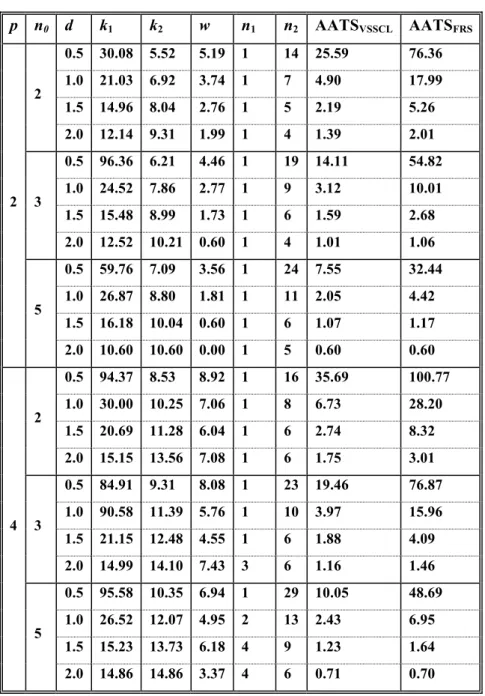
The results indicate that the proposed VP scheme with one warning limit performs well to the two-scaled VP (2SVP) scheme and furthermore it considers implementing considerations due to its fewer parameters and its one-scaled property. The differences between the two schemes are not much even for detecting small shifts. If varying the sampling intervals is not practical in the field, the VSSCL scheme is then an alternative to the VP T2 chart. Table 2 presents the results. If varying sample sizes is not desired, the VSICL scheme is recommended. Table 3 gives the optimal parameters of the VSICL scheme. With a comparison to the VSI scheme, varying the control limit improves the power of that chart. Our findings indicate that the VP scheme is more powerful than the VSICL and consequently VSI scheme in detecting small shifts; however, the differences between two schemes to detect moderate to large shifts are not significant. The surprising finding is that the
VSSCL scheme is more powerful than the VP scheme in detecting small mean shifts. This is discussed in the next section.
3. A numerical comparison between the different variable ratio sampling schemes
The practitioners are faced to a group of seven variable ratio sampling policies: VP, DWL, VSSCL, VSICL, VSSI, VSS and VSI. Each sampling scheme overcomes the FRS schemes (except in detecting large shifts) and can be used upon application considerations and the amount of the specific shift, which is of concern. Table 4 summarizes the comparison results between these schemes and provides information to help practitioners in selecting the most powerful scheme in order to have the maximum protection over a pre-determined value of the shift. The results are somewhat opposed to what we expected. Comparison results indicate that for small shifts (d≤ 0.5) the VSSCL scheme is superior to the DWL, VP, VSICL, VSSI, VSS and VSI schemes. The VP and then the DWL schemes show better performance than the others in detecting moderate shifts (0.5 < d ≤ 1.5). For detecting larger shifts (d >1.5) the VSICL and VSI schemes are good options. However, the differences between schemes in detecting large shifts are not significant, but due to their simplified structures can be recommended in practice.
According to Tables 1 - 4, it is clear that different schemes have different structures for detecting different magnitude of shifts in the process. So, when estimating the magnitude of shift is costly or a process is subject to multiple shifts, then it is recommended to apply a scheme that shows good performance for all shifts. We have to take into account that a different curve AATS versus d is obtained in function of selected value of d employed to optimize the power of the chart. After analyzing the diverse available options, Faraz and Parsian (2006)
showed that the optimum charts are obtained for d =0.75 and these charts generally
show a very good performance. Furthermore, as mentioned by Costa (1999), the parameter λ has minor influence on the AATS and hence on comparing results. Hence, in this section a comparison is made for the case p = 2, n0 = 2, h0 = 1 and λ =
0.01. Hence, the following charts are compared:
1. The VP T2 chart: k1 = 25.87; k2 = 6.51; w = 4.17; h1 = 1.13; h2 = 0.1; n1 =1
2. The DWL T2 chart: k= 10.60; wh = 1.27; wn = 5.20; h1 = 2.03; h2 = 0.1; n1 =1
and n2 =14.
3. The VSSCL T2 chart: k
1 = 25.14; k2 = 6.27; w = 4.41; h = 1; n1 =1 and n2
=10.
4. The VSICL T2 chart: k1 = 13.51; k2 =9.69; w = 1.14; h1 = 2.20; h2 = 0.1; and
n=2.
5. The VSSI T2 chart: k= 10.60; w = 4.71; h1 = 1.10; h2 = 0.1; n1 =1 and n2 =11.
6. The VSS T2 chart: k= 10.60; w = 5.48; h = 1; n1 =1 and n2 =15.
7. The VSI T2 chart with parameters k= 10.60; w = 0.63; h1 = 3.47; h2 = 0.1;
and n=2.
Figure 2 illustrates the comparison results when d differs from small to large shifts. The comparison shows that the VSICL and VSI schemes are unable to detects small to moderate shifts. These two schemes have a good power in detecting the shifts d ≥ 1.5. As Faraz and Parsian (2006) indicated, the DWL schemes is always a better option in detecting almost all process mean shifts while compared to the VSS, VSI and VSSI schemes, but when it comes to the VP and VSSCL T2 charts, other
schemes are dominated. In fact, adopting variable action limits provides a great improvement for the DWL and VSSI T2 charts. Even more, the VSSCL and VP schemes have smaller value of the parameter n2 with respect to the VSS, VSSI and
DWL schemes. In fact, letting the control limits vary between maximum and minimum values, smaller sample sizes are then required to detect out of control states, which is more economical too. By a comparison between the both VP and VSSCL schemes, we find out that the power of the VSSCL scheme, with not large differences, is almost smaller than the VP scheme and on the average the VSSCL scheme alarms almost 42 minutes sooner than the VP T2 chart in detecting small mean shifts (d = 0.5). On the other hand, the VP scheme shows better performance than the VSSCL in detecting moderate to large shifts (0.75 ≤ d ≤ 2) and on the average nearly 25 minutes sooner alarms. Of course, the VP scheme imposes some difficulties in application since the sampling intervals changes during the monitoring process. These adaptive changes in sampling intervals cause to increase the complexity of the chart. Hence, the VSSCL scheme, which always takes samples at fixed sampling intervals h0, is more convenient than the VP scheme. As a result, it
can be concluded that the VSSCL scheme is a statistically optimal sampling scheme
a very good performance when compared to the VP scheme in detecting for moderate to large shifts. Note that, the proposed VSSCL scheme does not require two charts with different measurement scales, since it only has one warning limit and that enables users to monitor the process in a single measurement scale.
4. Concluding remarks
The Hotelling'sT2control chart, a direct along of univariate shewhart X control
chart, is perhaps the most commonly used tool in industry for simultaneous monitoring of several quality characteristics. Recent studies have shown that applying variable ratio sampling (VRS) schemes yield faster detection of small to moderate shifts with respect to the FRS T2 control charts. Among existing schemes, the variable parameters (VP) has been proved to have a very good performance on detecting small to moderate shifts, however applying the VP T2 charts encounters some difficulties in the field. In this paper, we proposed an alternative to the VP T2 chart in that the sampling interval h, the Sample size n and control limit k vary between minimum and maximum values while keeping the warning line fixed over time. The proposed method uses only one measurement scale to overcome the applied difficulties of using two scales in the field. This idea is also applied to the VSS and VSI schemes to form the VSSCL and VSICL T2 charts. Through numerical comparisons between the seven existing VRS schemes in the literature, we show that the VSSCL scheme is statistically optimal and performs excellent for small shifts in process mean. Moreover, the VSSC T2 chart performs well to the VP T2 chart in detecting moderate to large shifts and that the VSSC T2 chat is a more popular scheme in practice than the VP charts due to its fewer parameters and ease of application. In fact, one may give up the merits of the VP scheme in detecting moderate to large shifts for the ease of application of the VSSCL scheme in the field.
Acknowledgment:
We’d like to thank and express our best gratitude to Islamic Azad University, Hamedan Branch, Hamedan, Iran and National Fund for Scientific Research (FNRS) organization, Brussels, Belgium that financially supported this research project. We also would like to acknowledge and extend our heartfelt gratitude to the anonymous
reviewers, the Editor and Editor in chief, all of whom helped us to improve this paper.
References
1) Amin, R.W. and Hemasinha R., The switching behavior of X-bar charts with variable sampling intervals, Communications in Statistics - Theory and Methods 22(1993) 2081 – 2102
2) Chen, Y. K.; Adaptive sampling enhancement for Hotelling’s T2 charts, European Journal of Operational Research 178 (2007) 841–857.
3) Chen, Y. K., Hsieh, K. L.: Hotelling's T2 charts with variable sample size and control limit. European Journal of Operational Research (2006) DOI:10.1016/j.ejor.2006.09.046. 4) Chengalur I.N., Arnold J.C. and Reynolds Jr, M.R., Variable sampling intervals for
multiparameter shewhart charts, Communications in Statistics - Theory and Methods 18(1989) 1769 – 1792. DOI: 10.1080/03610928908830000
5) Cinlar, E.: Introduction to stochastic process. Englewood Cliffs, NJ, Prentice Hall (1975). 6) Costa A.F.B., Vssi X-bar charts with sampling at fixed times, Communications in Statistics -
Theory and Methods 27(1998) 2853 – 2869.
7) Costa, A.F.B., Xbar Charts with variable parameters, Journal of Quality Technology, 31 (1999) 408-416.
8) Faraz, A. and Parsian, A., Hotelling’s T2 Control Chart with Double Warning Lines, Statistical paper, 43 (2006).
9) Faraz, A. and Moghadam, M. B., Hotelling’s T2 Control Chart with Two-State Adaptive Sample Size, Quality & Quantity, International Journal of methodology, DOI 10.1007/s11135-008-9167-x. 43 (2009) 903-913.
10) Faraz, A. and E. Saniga, A Unification and Some Corrections to Markov Chain Approaches to Develop Variable Ratio Sampling Scheme Control Charts, Statistical Papers, (2009) DOI 10.1007/s00362-009-0288-7.
11) Faraz, A., Kazemzade, R.B. and Saniga, E., Economic and Economical Statistical Design of Hotelling’s T2 Control Chart with Two-State Adaptive Sample Size. Journal of Statistical
Computation and Simulation, 80(12) (2010) 1299 – 1316. DOI: 10.1080/00949650903062574.
12) Faraz, A., Chalaki, K. and Moghadam M.B., On the properties of the Hotelling’s T2 Control Chart with VSI Scheme, Quality & Quantity, International Journal of methodology, 45(3)(2011) 579-586. DOI: 10.1007/s11135-010-9314-z
13) Faraz, A. and Saniga E., Economic and Economical Statistical Design of Hotelling’s T2 Control Chart with Double Warning Lines. Quality and Reliability Engineering International, 27(2)(2011) 125-139. DOI: 10.1002/qre.1095.
14) Faraz, A., Heuchenne, C. and Saniga E., Optimal T2 Control Chart with a Double Sampling Scheme – An Alternative to the MEWMA Chart. Quality and Reliability Engineering International, 28 (2012a) 751-760. DOI: 10.1002/qre.1268.
15) Faraz, A., R.B. Kazemzadeh, Parsian A., and Moghadam M.B., On the Advantages of Economically Designed Variable Sample Sizes and Sampling Intervals T2 Control Chart, Quality & Quantity, International journal of methodology. 46 (2012b) 1323-1336. DOI: 10.1007/s11135-010-9325-9.
16) Faraz, A., Celano, G., Heuchenne, C., Saniga, E. and Fichera, S. The variable parameters T2 chart with run rules, Statistical Papers, (2013a) DOI: 10.1007/s00362-013-0537-7.
17) Faraz, A., Heuchenne, C., Saniga, E., and Costa, A.F.B. Double Objective Economic Statistical Design of the VP T2 Control Chart: Wald’s identity approach. Journal of Statistical Computation and Simulation, (2013b). DOI:10.1080/00949655.2013. 784315 18) Hotelling H.: Multivariate quality control– Illustrated by the air testing of sample
bombsights. Techniques of Statistical Analysis, Eisenhart, C., Hastay, M.W., Wallis, W.A. (eds), New York: MacGraw-Hill (1947).
19) Seif, A., Faraz, A., Heuchenne, C. and Moghadam, M.B., Statistical Merits and Economic evaluation of the Hotelling’s T2Control Chart with variable sample sizes and control limits, Arabian Journal for Science and Engineering, 36 (2011a) 1461-1470. DOI: 10.1007/s13369-011-0124-y.
20) Seif, A., Faraz, A., Heuchenne, C., Saniga, E. and Moghadam, M.B., Economic- Statistical design of T2 control chart with the VSSC sampling schem, Journal of Applied Statistics, 38
21) Tornga C.C. and Lee P.H., The Performance of Double Sampling Control Charts Under Non Normality, Communications in Statistics - Simulation and Computation 38 (2009) 541-557. DOI:10.1080/03610910802571188
22) Torabian, M., Moghadam, M.B. and Faraz, A. , Economically designed Hotelling’s T2 Control Chart using VSICL schemes, Arabian Journal for Science and Engineering, 35 (2010) 251–263.
23) Lin, Y. The Variable Parameters X-bar Control Charts for Monitoring Autocorrelated Processes, Communications in Statistics - Simulation and Computation 38(2009) 729-749 DOI:10.1080/03610910802645339
Figures
Figure 1. A schematic VP T2 control chart
0.00 10.00 20.00 30.00 40.00 50.00 60.00 70.00 d AATS VP 26.88 9.33 4.72 3.11 2.31 1.80 1.45 DWL 41.18 10.90 5.38 3.56 2.56 1.95 1.58 VSSCL 26.16 9.52 5.10 3.57 2.83 2.38 2.07 VSICL 64.79 25.10 9.91 4.41 2.40 1.63 1.32 VSSI 48.22 12.69 5.50 3.58 2.63 2.01 1.57 VSS 44.72 12.80 6.69 4.68 3.54 2.78 2.23 VSI 66.10 26.21 10.58 4.90 2.87 2.13 1.85 0.50 0.75 1.00 1.25 1.50 1.75 2.00
Tables
Table 1. A Comparison between the VP , 2SVP and FRS schemes in accordance with
AATS performance for p =2 and 4, n0 =2, 3 and 5, h0 =1, α = 0.005 and λ = 0.01.
p n0 d k1 k2 w h1 h2 n1 n2 AATSVP AATS2SVP AATSFRS
2 2 0.5 32.64 5.99 4.70 1.10 0.10 1 11 26.29 24.43 76.36 1.0 22.32 7.35 3.30 1.22 0.10 1 6 4.47 4.36 17.99 1.5 15.31 8.47 2.29 1.43 0.10 1 4 1.66 1.66 5.26 2.0 11.09 9.82 2.33 1.42 0.10 1 4 0.93 0.93 2.01 3 0.5 42.45 6.36 4.31 1.12 0.10 1 18 14.32 13.45 54.82 1.0 25.45 8.37 2.26 1.44 0.10 1 7 2.69 2.6 10.01 1.5 13.01 9.16 1.86 1.60 0.10 1 6 1.08 1.08 2.68 2.0 10.60 10.60 2.20 1.46 0.10 1 7 0.69 0.69 1.06 5 0.5 80.11 7.36 3.28 1.22 0.10 1 21 7.64 6.41 32.44 1.0 23.63 9.04 1.58 1.77 0.10 1 10 1.48 1.4 4.42 1.5 10.60 10.60 1.73 1.67 0.10 1 10 0.72 0.72 1.17 2.0 10.60 10.60 2.18 1.47 0.10 1 13 0.56 0.56 0.60 4 2 0.5 48.53 9.49 7.90 1.10 0.10 1 11 38.09 37.78 100.77 1.0 32.15 10.62 6.65 1.17 0.10 1 7 6.45 6.39 28.20 1.5 21.68 11.85 5.31 1.32 0.10 1 4 2.23 2.23 8.32 2.0 16.42 12.55 5.76 1.26 0.10 2 3 1.15 1.15 3.01 3 0.5 96.98 9.49 7.90 1.10 0.10 1 21 20.02 19.88 76.87 1.0 31.86 11.65 5.47 1.30 0.10 1 8 3.70 3.70 15.96 1.5 17.34 12.27 5.53 1.29 0.10 2 5 1.38 1.38 4.09 2.0 15.30 13.34 6.73 1.17 0.10 3 4 0.79 0.79 1.46 5 0.5 83.07 10.57 6.70 1.17 0.10 1 26 10.25 10.14 48.69 1.0 20.16 11.93 5.33 1.32 0.10 3 10 1.93 1.96 6.95 1.5 15.11 14.08 6.00 1.23 0.10 4 9 0.83 0.83 1.64 2.0 14.86 14.86 7.80 1.10 0.10 4 14 0.59 0.59 0.70
Table 2. A Comparison between the VSSCL and FRS schemes in accordance with AATS
performance for p =2 and 4, n0 =2, 3 and 5, h0 =1, α = 0.005 and λ = 0.01.
p n0 d k1 k2 w n1 n2 AATSVSSCL AATSFRS 2 2 0.5 30.08 5.52 5.19 1 14 25.59 76.36 1.0 21.03 6.92 3.74 1 7 4.90 17.99 1.5 14.96 8.04 2.76 1 5 2.19 5.26 2.0 12.14 9.31 1.99 1 4 1.39 2.01 3 0.5 96.36 6.21 4.46 1 19 14.11 54.82 1.0 24.52 7.86 2.77 1 9 3.12 10.01 1.5 15.48 8.99 1.73 1 6 1.59 2.68 2.0 12.52 10.21 0.60 1 4 1.01 1.06 5 0.5 59.76 7.09 3.56 1 24 7.55 32.44 1.0 26.87 8.80 1.81 1 11 2.05 4.42 1.5 16.18 10.04 0.60 1 6 1.07 1.17 2.0 10.60 10.60 0.00 1 5 0.60 0.60 4 2 0.5 94.37 8.53 8.92 1 16 35.69 100.77 1.0 30.00 10.25 7.06 1 8 6.73 28.20 1.5 20.69 11.28 6.04 1 6 2.74 8.32 2.0 15.15 13.56 7.08 1 6 1.75 3.01 3 0.5 84.91 9.31 8.08 1 23 19.46 76.87 1.0 90.58 11.39 5.76 1 10 3.97 15.96 1.5 21.15 12.48 4.55 1 6 1.88 4.09 2.0 14.99 14.10 7.43 3 6 1.16 1.46 5 0.5 95.58 10.35 6.94 1 29 10.05 48.69 1.0 26.52 12.07 4.95 2 13 2.43 6.95 1.5 15.23 13.73 6.18 4 9 1.23 1.64 2.0 14.86 14.86 3.37 4 6 0.71 0.70
Table 3. A Comparison between the VSICL and FRS schemes in accordance with AATS
performance for p =2 and 4, n0 =2, 3 and 5, h0 =1, α = 0.005 and λ = 0.01.
p n0 d k1 k2 w h1 h2 AATSVSICL AATSFRS
2 2 0.5 87.41 9.77 0.84 2.75 0.10 65.99 76.36 1.0 13.80 9.59 1.22 2.09 0.10 9.90 17.99 1.5 12.96 9.22 1.80 1.63 0.10 2.28 5.26 2.0 11.69 8.93 2.86 1.29 0.10 1.01 2.01 3 0.5 13.15 9.73 1.14 2.19 0.10 42.53 54.82 1.0 13.61 9.44 1.41 1.90 0.10 4.72 10.01 1.5 12.05 8.99 2.47 1.38 0.10 1.24 2.68 2.0 11.01 9.01 4.09 1.14 0.10 0.70 1.06 5 0.5 13.59 9.68 1.14 2.19 0.10 21.49 32.44 1.0 12.74 9.16 1.94 1.56 0.10 1.92 4.42 1.5 11.10 8.97 3.86 1.16 0.10 0.73 1.17 2.0 10.60 10.60 4.71 1.10 0.10 0.56 0.60 4 2 0.5 17.64 14.16 2.43 2.77 0.10 88.25 100.77 1.0 18.85 14.09 2.36 2.87 0.10 16.63 28.20 1.5 18.22 13.62 3.28 1.97 0.10 3.62 8.32 2.0 16.70 13.11 4.68 1.44 0.10 1.35 3.01 3 0.5 18.08 14.18 2.29 2.98 0.10 62.36 76.87 1.0 18.78 13.91 2.69 2.44 0.10 7.93 15.96 1.5 17.19 13.25 4.19 1.57 0.10 1.75 4.09 2.0 15.68 12.97 6.18 1.21 0.10 0.83 1.46 5 0.5 18.57 14.18 2.22 3.09 0.10 34.29 48.69 1.0 17.99 13.52 3.48 1.85 0.10 2.97 6.95 1.5 15.82 12.97 5.91 1.24 0.10 0.88 1.64 2.0 14.97 14.07 7.91 1.10 0.10 0.59 0.70
Table 4. A Comparison between the VP, DWL, VSSCL, VSICL, VSSI, VSS, VSI and FRS
schemes in accordance with AATS performance for p =2 and 4, n0 =2, 3 and 5, h0 =1, α
= 0.005 and λ = 0.01.
p n0 d VP DWL VSSCL VSICL VSSI VSS VSI FRS
2 2 0.5 26.29 37.67 25.59* 65.99 48.22 39.97 66.10 76.36 1.0 4.47* 4.72 4.90 9.90 5.18 5.88 10.54 17.99 1.5 1.66* 1.73 2.19 2.28 1.83 2.38 2.43 5.26 2.0 0.93* 0.98 1.39 1.01 1.17 1.43 1.04 2.01 3 0.5 14.32 18.71 14.11* 42.53 20.98 19.79 43.87 54.82 1.0 2.69* 2.69* 3.12 4.72 3.06 3.61 5.06 10.01 1.5 1.08* 1.19 1.59 1.24 1.57 1.69 1.29 2.68 2.0 0.69* 0.69* 1.01 0.69* 1.15 1.02 0.69* 1.06 5 0.5 7.64 9.09 7.55* 21.49 9.45 9.72 22.53 32.44 1.0 1.48 1.46* 2.05 1.92 2.21 2.27 2.03 4.42 1.5 0.72* 0.72* 1.07 0.73 1.51 1.09 0.74 1.17 2.0 0.56* 0.56* 0.60 0.56* 1.15 0.60 0.56* 0.60 4 2 0.5 38.09 54.97 35.69* 88.25 73.12 57.36 89.55 100.77 1.0 6.45* 6.92 6.73 16.63 7.75 8.29 17.38 28.20 1.5 2.23* 2.27 2.46 3.62 2.38 3.03 3.85 8.32 2.0 1.15* 1.17 1.23 1.35 1.17 1.76 1.40 3.01 3 0.5 20.02 26.94 19.48* 62.36 33.65 27.92 63.67 76.87 1.0 3.71* 3.84 3.81 7.93 4.15 4.69 8.39 15.96 1.5 1.38* 1.38* 1.42 1.75 1.42 2.00 1.84 4.09 2.0 0.79* 0.79* 0.84 0.83 0.79* 1.16 0.84 1.46 5 0.5 10.25 12.66 9.96* 34.29 13.12 13.13 35.38 48.69 1.0 1.93 1.93 1.80* 2.97 2.07 2.70 3.16 6.95 1.5 0.83* 0.83* 0.90 0.88 0.87 1.24 0.90 1.64 2.0 0.59* 0.59* 0.70 0.59* 0.63 0.71 0.59* 0.70