STEREO AMBIGUITY INDEX FOR SEMI-GLOBAL MATCHING
Mathias Paget, Jean-Philippe Tarel
Universit´e Paris-Est, LEPSIS, IFSTTAR,
F-77447 Marne-la-Vall´ee, France
Pascal Monasse
LIGM (UMR 8049), ´
Ecole des Ponts, UPE,
Champs-sur-Marne, France
ABSTRACT
Stereoscopic reconstruction is important to automatic vision sys-tems. As an intermediate step, estimating this reconstruction is not enough for good performance of the whole system, and its uncer-tainty must be characterized. Several methods propose unceruncer-tainty indexes based on specific data features, thus incomplete, while oth-ers are based on learning. We propose a simple index, named am-biguity index, taking into account both data and regularization, and derived directly from the optimization process. Exploiting properties of dynamic programming, this index is related to the posterior vari-ance of the solution when the Semi-Global Matching (SGM) algo-rithm is used for stereo reconstruction. To illustrate its interest, im-provements in refining stereo reconstruction are shown on the KITTI datasets when the index is used.
Index Terms— Stereo reconstruction, Discrete optimization, Dynamic Programming, Semi-Global Matching, Uncertainty index
1. INTRODUCTION
A robust and accurate perception of the environment is required for advanced driver assistance systems (ADAS) to perform driving tasks. When only cameras are used for perception, many driving tasks, where the system extracts high-level information from low-level image information, are known to challenge computer vision systems. To face these difficult and complex problems, tasks are usually decomposed into a chain of sub-problems, each sub-problem being handled by an image or computer vision process. In such an approach, the output of each process is the input of another one. Of-ten, each process consists in the minimization of an energy. The advantage of the decomposition into sub-problems is that the prop-agated information is reduced along the chain; however the risk is to reduce the propagated information too drastically and to lead to inconsistent results. To solve this issue it is necessary to propagate uncertainty information in addition to the estimated result to allow the next process to integrate it in its processing. We focus here on stereoscopic reconstruction of road scenes.
When the input noise is Gaussian and the problem is linear and well-posed, the uncertainty of the output is a Gaussian function char-acterized by the covariance matrix of the output. This covariance matrix can be formally derived from the minimized energy. When the input noise is not Gaussian, or when the problem is non-linear, the uncertainty of the output can only be approximated by a Gaussian function. The covariance matrix is voluminous for large number of parameters. Thus, only problems with a reduced number of param-eters, such as for instance camera calibration, can be handled, but not stereo reconstruction, where the number of parameters is usually over one million. Rather than estimating the full covariance matrix of the output, it was thus proposed to estimate an uncertainty index per pixel based on the data features which are known to hinder the
resolution of the problem, such as texture-less regions, repetitive pat-terns [1]. The difficulty of this approach is that it is hard to capture the effect of data on the estimated solution due to the usual regu-larization term, such as the logarithm of the prior probability of the depth map, used during stereo reconstruction minimization.
This is why it was recently proposed to learn confidence on the solution. Confidence has to be understood as a prediction of an error on matching over a given threshold. It is learned from data, data cost and estimated disparity map features [2, 3, 4] and additionally from final energy cost [5]. These approaches require supervised learning and a large ground-truth database, so we investigate the possibility of building an uncertainty index from the energy and the optimization process only, in order to estimate the ambiguity of the solution. It appears that optimization methods based on Dynamic Programming (DP), such as the discrete optimization method Semi-Global Match-ing (SGM) [6], have very interestMatch-ing properties, which allows us to estimate easily an index on the solution. This so called ambiguity index comes from intermediate costs computed during the optimiza-tion and needs a reduced amount of computaoptimiza-tion to be obtained. The proposed ambiguity index is evaluated in several experiments, show-ing its interest. In particular, we use it to refine the stereo reconstruc-tion and show how it can be used to improve results.
2. STEREO RECONSTRUCTION
The used stereo reconstruction algorithm is a simplified version of a recent method [7], assuming input images are already in rectified geometry. Following [8], we describe the algorithm split into match-ing cost computation and cost aggregation in Sec. 2.1, optimization in Sec. 2.2 and refinement in Sec. 2.3.
2.1. Matching Cost and Aggregation
In the rectified geometry, object depth is easily parameterized by the horizontal difference in position between its left and right pro-jections, the so-called disparity. Stereo reconstruction problem is usually set as the minimization, with respect to the disparity image, of an energy which is a function of the left and right images. The Bayesian approach provides ways to derive this energy from a sta-tistical model of the stereo reconstruction problem. The classic form of the energy is E(D) =X p∈P Data(p, dp) + X (p,q)∈N Prior(dp, dq), (1)
where D = (dp) is the disparity map with dpthe disparity of the
pixel p, P is the pixel set, N the set of neighbor pairs of pixels. The data term Data describes how data agrees with the solution and the prior term Prior, used as a regularizer, encodes the wanted properties
of the solution. In our case, Data is set to the census dissimilar-ity [9] between left and right pixel patches. The census is computed on a 5 × 5 pixel window and the advantage is its invariance to an increasing function on the intensities, so it can handle photometric calibration differences between the two images and partially pertur-bations due to aspect differences depending on the view angle. Like in [10], cross-based aggregation is performed on the data cost. By smoothing the data cost in regions of homogeneous intensities, the noise is reduced in the data cost.
The term Prior is set to a function of the disparity difference, assuming that two neighbor pixels frequently have the same depth (also called fronto-parallel prior). The assumption on the data term is not quite valid due to occlusion, reflections and specularities, as well as on the prior term due to non-frontal surfaces such as the road and lateral buildings. Attests at perform more accurate modeling, for instance to handle occlusion [11, 12] or regularization with higher order prior [13], make it more difficult to optimize energies. For this reason, simple energies are often preferred and erroneous pixels of the solution are post-processed. In practice, Prior is set to:
Prior(i, j) = 0 if i = j, Prior(i, j) = P1 if |i − j| = 1,
Prior(i, j) = P2 otherwise,
(2)
where 0 ≤ P1 ≤ P2 are fixed parameters. It thus behaves
al-most like a P ott regularization function, yet is more permissive for slow disparity variations. This allows better handling of road scenes where there are non-frontal planes.
2.2. Semi-Global Matching Optimization
The energy (1) is a 2D first order Markov Random Field (MRF). Global optimization of such an energy is difficult, so approxi-mate optimization algorithms have been proposed. In Semi-Global Matching (SGM) introduced by Hirschm¨uller [6], the original en-ergy is decomposed in many 1D energies whose each global opti-mum can be found. SGM thus consists in minimizing along “arms” around each considered pixel by Dynamic Programming (DP). For each pixel and vector direction v, a 1D energy Cvis computed using
the following recursion rule: Cv(p, d) = Data(p, d) +
min
d0 Cv(p − v, d 0
) + Prior(d, d0). (3) The original SGM is performed along R = 16 directions v. We consider only R = 4 directions as in [7], since fostering horizontal and vertical directions in the optimization achieves better results for vertical and horizontal scene objects. The energies Cvare added at
the current pixel and the estimate is selected at the minimal value of this energy over disparities:
SGM (p, d) =X v Cv(p, d) − (R − 1)Data(p, d) dp= arg min d SGM (p, d). (4)
Because of the 1D decomposition, each pixel solution is obtained independently and thus the smoothness of the solution is not guaran-teed, despite the regularization term, leading to artifacts. Smoothing the data cost with cross based aggregation reduces these artifacts.
2.3. Left-Right Consistency (LRC) refinement
Since the model is not always valid, in particular at occlusions, an additional prior is introduced during post-processing, the so-called Left-Right Consistency (LRC) on disparities [14]. The idea is to check that for the same object point, the disparity in the left and right images are opposites. LRC check consists in comparing the disparity of a given pixel to the disparity at the corresponding position in the other image. Three pixel categories are thus defined:
if |Dl(p) + Dr(p − Dl(p))| ≤ 1 correct,
else if |d + Dr(p − d)| ≤ 1, for some d 6= Dl(p), mismatch,
otherwise occlusion. (5) A refinement on the result is performed based on the LRC cate-gory [7]: for “correct” pixels, the solution value is not modified; for any “occlusion” pixel, the value is copied from the closest “correct” pixel at its left, thus occluded pixels are set to the background. For “mismatch” pixels, the value is set to the median value of the nearest “correct” neighbors in 8 directions (originally 16).
3. AMBIGUITY INDEX 3.1. Posterior Variance for SGM solution
The a priori variance is related to the data cost only, it does not pro-vide useful information on the solution. This is why well selected features from input data were proposed to partially characterize the data uncertainty [1]. As the estimated solution is an agreement be-tween data and prior costs, it is quite hard to derive all the good features. The posterior variance of the estimated solution is a bet-ter characbet-terization, since it takes into account data and prior costs. However, its estimation for a 2D MRF such as energy (1) is a very complex task. Indeed, the posterior covariance is a quadratic approx-imation of the shape of the energy (1) around the obtained solution which is assumed at a local minimum of this energy. Due to the large number of parameters, the computation of this quadratic approxima-tion is intractable.
Since we are using SGM optimization, we work on the SGM cost. As recalled, the SGM optimization decomposes and approx-imates the 2D problem into many 1D problems. We exploit one important property of DP: each value in the DP final cost, thus after DP optimization, is the minimal energy of the original problem with an extra constraint on the solution. For SGM, this implies that each value of the SGM final cost is the minimum value of the following sub-problem: considering the set Xpof pixels within the
horizon-tal and vertical “arms” from the pixel p, the final cost SGM (p, d) is equal to the minimum cost over Xp, with the constraint that the
disparity value at p equals d. More formally: SGM (p, d) = min dx,x∈Xp|dp=d{ X x∈Xp Data(x, dx) + X (x,y)∈N ∩X2 p Prior(dx, dy)}. (6)
The SGM final cost can be seen as an approximation of the energy (1) where each final pixel disparity becomes independent of the oth-ers. This allows to disregard the covariance between different pixels and to focus only on the pixel posterior variance of the SGM solu-tion. The latter, our ambiguity index, is estimated as the size of the final SGM valleys along disparities:
Index(p) =X
d
where1 is the characteristic function witch returns 1 if argument is true and 0 if argument is false, T1is a fixed positive threshold. The
minimum index value of one means that there is no ambiguity. From experiments, the profile of the final SGM cost is usually observed with a single valley where the model is valid. Counting values un-der a threshold allows to take into account multiple valley where a energy profile is more complex. The proposed index looks similar to the perturbation measure [15] proposed in the context of plane-sweeping stereo. In practice, T1 is set at a factor of the P2 value
used in the regularization term. This link between T1and P2 leads
to invariance of the index when a scale factor is applied to the energy. Notice also that the estimated result and ambiguity index derive from the same energy, so a change in the energy affects both of them. The extra cost for ambiguity index computation is much reduced. 3.2. Index Integration Into the Stereo Process
A way to evaluate the index relevance is to use it to refine the recon-struction and to test whether the solution is improved. We propose two possibilities. The first one is a post-processing similar to LRC filtering (Sec. 2.3), where pixels whose index is under a threshold T2 are tagged as “correct” label. As the index cannot distinguish
“mismatch” and “occlusion”, all other pixels are handled as “mis-match” and set to the median of the nearest “correct” neighbors in 8 directions.
The confidence obtained from learning has been used as a weight in the data cost [3] or regularization cost [2] to balance data and regularization terms. In [4], an extra regularization term is added de-pending on the confidence value. Our second investigated possibility is to reweight the data term using the inverse of the index:
New Data(p, d) = KData(p, d)
Index(p) , (8) where K is a constant maintaining global balance between data and regularization terms. Then, a second SGM optimization is performed with this new data cost.
4. EXPERIMENTS
We use stereo rectified image pairs of the KITTI 2012 [16] and KITTI 2015 [17] datasets. Not being learned, our index is only eval-uated on training sets with ground-truth. We use the criterion of KITTI on the “Non-occulted” ground-truth pixels witch are forced to stand into the two cameras’ field of view. The same parameters are used for KITTI 2012 and 2015, color images of KITTI 2015 being converted to grey scale before processing. Regularization parame-ters are set as P1= 1.2 and P2= 23.
4.1. Ambiguity Index as an Occlusion Prediction
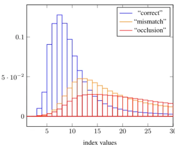
Where the reconstruction model is not valid, we expect data not to agree with the model and thus the solution to show a high ambiguity index value, especially at occlusions. We thus compare the ambigu-ity index with the LRC pixel label which is used as a ground-truth. This ground-truth can be discussed but seems to be the one more sig-nificant, presently. Fig. 1 shows the result on KITTI 2012 training set. Despite the overlap between the three histograms, considering ambiguity index as a non “correct” label predictor gives a 77.7% recall for a 50% precision, thus an over detection by a factor two. This is interesting, as our ambiguity index has not been designed specifically to be an occlusion predictor.
5 10 15 20 25 30 0 5 · 10−2 0.1 index values “correct” “mismatch” “occlusion”
Fig. 1: Normalized histograms of index values for the three pixel labels (“correct”, “mismatch”, “occlusion”) after LRC for all the left images of KITTI 2012 training set. The “correct” mode is at index = 7, whereas “mismatch” mode is at index = 12 and “oc-clusion” mode at index = 13.
Error rate (%) Before After KITTI2012 / KITTI2015 LRC refinement LRC refinement Original (without index) 6.12 / 5.23 5.13 / 4.48 Refinement 1 5.38 / 4.77 4.85 / 4.35 Refinement 2 5.25 / 4.55 4.59 / 4.04 Table 1: Average percentage of disparities below 3 pixels error from the “non-occulted” ground truth KITTI 2012 and KITTI 2015 train-ing sets. Refinement 1 is LRC pixel refinement whose index is over 20. Refinement 2 divides the data cost by the ambiguity index before a second SGM optimization.
We now consider pixels with an index value higher than the threshold we set at T2 = 20 to be a “mismatch” in the first
refine-ment method proposed in Sec. 3.2. Error rates with the ground-truth are shown in Tab. 1. Results before and after standard LRC refine-ment are also shown. The error rates with LRC and Refinerefine-ment 1 alone are similar and this suggests that the ambiguity index is a good predictor of non “correct” pixels. When the LRC refinement is ap-plied to the output of Refinement 1, results slightly improve. This suggests that if LRC and Refinement 1 have a shared effect, they are also slightly complementary.
Fig. 2 shows the values of the left and right ambiguity indexes for pixels labeled “correct” by LRC. Notice there is a good cor-respondence between left and right ambiguity indexes. Therefore, when disparities are consistent, ambiguity index is also consistent between left and right images.
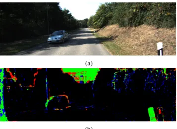
Fig .3 shows pixels detected with a high ambiguity index with respect to LRC labels (“correct” or non “correct”): true positive in green, false positive in red, false negative in blue and true negative in black. Most occlusions are detected. Under-detection concerns thin objects or small discontinuities, and over-detection is mostly due to objects seen in the right image but not in the left image.
4.2. Ambiguity Index as Data Uncertainty
We tested the second refinement method proposed in Sec .3.2 with K = 15. Results are reported in the last line of Tab. 1. What was ob-served with Refinement 1 is confirmed with Refinement 2, with the
0 5 10 15 0
5 10 15
left index values
right inde x v alues 0 1 2 3 ·106
Fig. 2: For all “correct” matches of the KITTI 2015 training set, co-occurrence of ambiguity index value in the left and the right image are shown. Each element of the matrix represents a number of pixel couple having a given index value at the left and the right image positions. Notice how left and right ambiguity index are close when disparity matches.
(a)
(b)
Fig. 3: (a) Left image 056 of KITTI 2015 training set, (b) shows pix-els detected as ambiguous (threshold at 15) with respect to LRC ref-erence: true positive in green, over detection in red, under-detection in blue, true negative in black.
difference that combining LRC and Refinement 2 leads to even bet-ter improvements. On KITTI 2012, the obtained error rate is ranked 37, and for KITTI 2015, it is ranked between 10 to 15 (in January 2017) which is encouraging knowing that a better data cost (based on learning) than our simple census could be used.
A reconstruction result with and without the use of the index is shown in Fig. 4, for illustration. Notice how the disparity map is improved on the tramway windows. The ambiguity index detects reflections on the tramway windows, saturated pixels in the sky and occlusion at the left of the car.
5. CONCLUSION
Our goal was to characterize the uncertainty of the disparity map estimated during stereo reconstruction process, a necessary but dif-ficult task to perform. We proposed an ambiguity index designed to approximate the variance of every pixels of the estimated disparity
(a) Left image
(b) Ambiguity index image
(c) Left disparity without index
(d) Left disparity with index weighting
Fig. 4: Results on image 144 of KITTI 2015 training set (a): Am-biguity index in (b), (c) disparity map without using the index, and (d) using the index. Higher index is whiter in (b). Notice how re-construction is improved on the tramway windows between (c) and (d).
map. This ambiguity index can only be computed when Dynamic Programming is used to solve the stereo reconstruction problem, as it is the case for the well known SGM optimization. In the experi-ments, it was shown that the proposed index has higher values where the data does not match with the model, for example in case of oc-clusion and in presence of specularities. This allows using the am-biguity index to improve the results by a post-processing, as shown experimentally with two proposed refinement methods on the KITTI 2012 and KITTI 2015 datasets. The proposed index can be also used for other kinds of problems, provided the optimization is based on Dynamic Programming.
6. REFERENCES
[1] Xiaoyan Hu and Philippos Mordohai, “A quantitative evalu-ation of confidence measures for stereo vision,” IEEE Trans-actions on Pattern Analysis and Machine Intelligence, vol. 34, no. 11, pp. 2121–2133, 2012.
[2] Aristotle Spyropoulos, Nikos Komodakis, and Philippos Mor-dohai, “Learning to detect ground control points for improv-ing the accuracy of stereo matchimprov-ing,” in Proceedimprov-ings of the
IEEE Conference on Computer Vision and Pattern Recogni-tion, 2014, pp. 1621–1628.
[3] Min-Gyu Park and Kuk-Jin Yoon, “Leveraging stereo match-ing with learnmatch-ing-based confidence measures,” in Proceed-ings of the IEEE Conference on Computer Vision and Pattern Recognition, 2015, pp. 101–109.
[4] Akihito Seki and Marc Pollefeys, “Patch based confidence pre-diction for dense disparity map,” in British Machine Vision Conference (BMVC), 2016, vol. 10.
[5] Ralf Haeusler, Rahul Nair, and Daniel Kondermann, “Ensem-ble learning for confidence measures in stereo vision,” in Pro-ceedings of the IEEE Conference on Computer Vision and Pat-tern Recognition, 2013, pp. 305–312.
[6] Heiko Hirschm¨uller, “Stereo processing by semiglobal match-ing and mutual information,” IEEE Transactions on pattern analysis and machine intelligence, vol. 30, no. 2, pp. 328–341, 2008.
[7] Jure Zbontar and Yann LeCun, “Stereo matching by train-ing a convolutional neural network to compare image patches,” Journal of Machine Learning Research, vol. 17, no. 1-32, pp. 2, 2016.
[8] Daniel Scharstein and Richard Szeliski, “A taxonomy and eval-uation of dense two-frame stereo correspondence algorithms,” International journal of computer vision, vol. 47, no. 1-3, pp. 7–42, 2002.
[9] Ramin Zabih and John Woodfill, “Non-parametric local trans-forms for computing visual correspondence,” in European con-ference on computer vision. Springer, 1994, pp. 151–158. [10] Ke Zhang, Jiangbo Lu, and Gauthier Lafruit, “Cross-based
local stereo matching using orthogonal integral images,” IEEE Transactions on Circuits and Systems for Video Technology, vol. 19, no. 7, pp. 1073–1079, 2009.
[11] Vladimir Kolmogorov and Ramin Zabih, “Computing visual correspondence with occlusions using graph cuts,” in Com-puter Vision, 2001. ICCV 2001. Proceedings. Eighth IEEE In-ternational Conference on. IEEE, 2001, vol. 2, pp. 508–515. [12] Vladimir Kolmogorov, Pascal Monasse, and Pauline Tan,
“Kolmogorov and Zabihs graph cuts stereo matching algo-rithm,” Image Processing On Line, vol. 4, pp. 220–251, 2014, https://doi.org/10.5201/ipol.2014.97. [13] Rene Ranftl, Stefan Gehrig, Thomas Pock, and Horst Bischof,
“Pushing the limits of stereo using variational stereo estima-tion,” in Intelligent Vehicles Symposium (IV), 2012 IEEE. IEEE, 2012, pp. 401–407.
[14] Xing Mei, Xun Sun, Mingcai Zhou, Shaohui Jiao, Haitao Wang, and Xiaopeng Zhang, “On building an accurate stereo matching system on graphics hardware,” in Computer Vision Workshops (ICCV Workshops), 2011 IEEE International Con-ference on. IEEE, 2011, pp. 467–474.
[15] Paul Merrell, Amir Akbarzadeh, Liang Wang, Philippos Mor-dohai, Jan-Michael Frahm, Ruigang Yang, David Nist´er, and Marc Pollefeys, “Real-time visibility-based fusion of depth maps,” in Computer Vision, 2007. ICCV 2007. IEEE 11th In-ternational Conference on. IEEE, 2007, pp. 1–8.
[16] Andreas Geiger, Philip Lenz, Christoph Stiller, and Raquel Ur-tasun, “Vision meets robotics: The kitti dataset,” The Interna-tional Journal of Robotics Research, vol. 32, no. 11, pp. 1231– 1237, 2013.
[17] Moritz Menze and Andreas Geiger, “Object scene flow for autonomous vehicles,” in Conference on Computer Vision and Pattern Recognition (CVPR), 2015.