Caractérisation des habitats d'alimentation du goéland à bec cerclé dans le sud du Québec

CARACTÉRISATION DES HABITATS D'ALIMENTATION DU GOÉLAND À BEC CERCLÉ DANS LE SUD DU QUÉBEC

MÉMOIRE PRÉSENTÉ COMME EXIGENCE PARTIELLE DE LA MAITRISE EN BIOLOGIE

PAR

MARTIN PATENAUDE-MONETTE

UNIVERSITÉ DU QUÉBEC À MONTRÉAL Service des bibliothèques

Avertissement

La diffusion de ce mémoire se fait dans le' respect des droits de son auteur, qui a signé le formulaire Autorisation de reproduire et de diffuser un travail de recherche de cycles supérieurs (SDU-522 - Rév.ü1-2üü6). Cette autorisation stipule que «conformément à l'article 11 du Règlement no 8 des études de cycles supérieurs, [l'auteur] concède à l'Université du Québec

à

Montréal une licence non exclusive d'utilisation et de publication de la totalité ou d'une partie importante de [son] travail de recherche pour des fins pédagogiques et non commerciales. Plus précisément, [l'auteur] autorise l'Université du Québec

à

Montréal

à

reproduire, diffuser, prêter, distribuer ou vendre des copies de [son] travail de recherche

à

des fins non commerciales sur quelque support que ce soit, y compris l'Internet. Cette licence et cette autorisation n'entraînent pas une renonciation de [la] part [de l'auteur]

à

[ses] droits moraux ni à [ses] droits de propriété intellectuelle. Sauf entente contraire, [l'auteur] conserve la liberté de diffuser et de commercialiser ou non ce travail dont [il] possède un exemplaire.»

bec cerclé (Laros delawarensis) du Sud du Québec m'a servi de modèle d'étude. Ce mémoire

est divisé en trois parties, dont une introduction générale, un chapitre principal sous forme d'article scientifique et une conclusion générale. Le chapitre principal a été rédigé en anglais avec la collaboration de mon directeur de maîtrise, Jean-François Giroux, de l'Université du Québec à Montréal, et de mon codirecteur de maîtrise, Marc Bélisle, de l'Université de Sherbrooke. Cet article sera soumis à la revue Journal of Animal Ecology. J'ai assumé

l'élaboration du projet, la récolte des données durant 2 saisons, la compilation et l'analyse des données ainsi que la rédaction de la première version et des versions subséquentes du mémoire. Jean-François Giroux a assuré la supervision de la collecte des données, des analyses de données et de l'interprétation des résultats. Marc Bélisle a participé à l'élaboration des protocoles pour la collecte de données, aux analyses statistiques et à l'interprétation des résultats. Ils ont tous les deux révisé différentes versions du mémoire.

Je tiens à remercIer en prenuer lieu mon directeur de recherche, Jean-François Giroux, pour son aide et ses encouragements. Il sait mettre sa grande expérience en recherche au service de ses étudiants, tout en leur laissant la liberté d'innover. Je lui suis reconnaissant de m'avoir offert de participer au démarrage d'un nouveau projet de recherche, une expérience des plus stimulantes. Je remercie également mon codirecteur, Marc Bélisle. Son sens critique, de même que son pragmatisme, ont été précieux pour orienter ce projet d'envergure. Ses conseils statistiques ont aussi été précieux pour s'assurer de la rigueur des analyses.

Je suis aussi très reconnaissant envers nos deux techniciens de terrain, Francis St­ Pierre et Mathieu Tremblay. Sans eux et leur organisation logistique du terrain, la collecte de données aurait été impossible. Forts de leur expérience, ils ont aussi fourni de précieux conseils lors de l'élaboration des protocoles de terrain, pour en assurer la rigueur et

iv

l'efficacité. Ils nous ont aussi pennis d'innover lors des captures et du marquage des oiseaux. Je tiens aussi à remercier particulièrement Mathieu Tremblay pour le travail de dissection et de tri de bols alimentaires. Un travail ardu et peu ragoûtant, mais essentiel. Merci aussi à Geneviève Turgeon, Ericka Thiériot, Jenny Guillemette et Valentin Nivet-Mazerolles pour leur contribution au tri des bols alimentaires.

Je tiens à remercier mes collègues de laboratoire, François Racine, Ericka Thiériot, Catherine Pilotte, Cécile Girault et Florent Lagarde pour tous leurs précieux conseils et les discussions enrichissantes. Je remercie François Racine, Ericka Thiériot et Cécile Girault pour leur aide sur le terrain. Je suis reconnaissant envers Cécile Girault pour ses conseils pour les analyses statistiques et géomatiques. Je remercie Catherine Pilotte de m'avoir accompagné lors des congrès de l'ACFAS et de la SOc. Je suis aussi reconnaissant envers Mélanie Desrochers, géomaticienne au Centre d'étude de la forêt, pour son aide en géomatique. Je voudrais aussi souligner les précieux conseils que m'a apportés Simon Benhamou lors du calcul du temps de résidence. Je suis aussi reconnaissant envers Regina Zamojska pour les analyses calorimétriques.

J'aimerais remercier les stagiaires de terrain qui m'ont aidé lors du projet: Geneviève Turgeon, Philippe Joyal, Claudie Landry, Catherine Bessette et Clotilde Pialat. Je tiens aussi à remercier les personnes suivantes pour leur collaboration au projet: Pierre Brousseau du Service canadien de la faune, Pierre Molina de Services environnementaux Faucon, Simon Mercier de Waste Management et Sandra Messih de Chamard et associés. Je suis aussi reconnaissant envers Giacomo Dell'omo et son équipe. Malgré un service à la clientèle hasardeux, je n'aurais pas pu obtenir des résultats aussi intéressants sans le consignateur de données GPS qu'ils ont conçu.

Je remercie Marie-Pier Léger-St-Jean pour la révision de mon anglais écrit. Je suis également reconnaissant envers Olivier Deshaies, Sébastien Auger, Émilie Chalifour, Émilie d'Astous et David Lévesque qui ont partagé à un moment ou un autre mon parcours académique et avec qui j'ai eu des conversations enrichissantes sur l'écologie, la recherche

universitaire, les statistiques et l'épistémologie. Je remercie mes parents pour leur soutien et leur PC sous Windows, précieux pour conununiquer avec les balises GiPSy. Je suis aussi très reconnaissant envers Frédérique Nadeau-Marcotte, ma compagne de vie, pour son soutien, ses encouragement et sa très grande patience. Finalement, je désire exprimer mes remerciements les plus sincères envers les dizaines de goélands manipulés lors du projet, qui n'ont rien demandé et qui ont parfois été sacrifiés pour la science.

T ABLES DES MATIÈRES

AVANT-PROPOS iii

LISTE DES FIGURES viii

LISTE DES TABLEAUX x

RESUME 1

INTRODUCTION 3

Sélection d'habitats 3

Écologie du déplacement 5

Complémentarités des approches analytiques 6

Populations de Laridés 7

Nuisances attribuées aux Laridés 8

CHAPITREI

FORAGING MOVEMENTS OF BREEDING RH,rG-BILLED GULLS IN A

HETEROGENEOUS LANDSCAPE: WHICH HABITAT IS THE BEST? ;." 1-1

SlTMMARy Il 1.1 Introduction 13 1.2 Methods 16 1.2.1 Study area 16 1.2.2 Telemetry 17 1.2.3 Gull Surveys 18

1.2.4 Diet and calorimetrie analyses 19

1.3 Data analysis 20

1.3.1 Telemetry 20

1.3.2 Resource selection function 21

1.3.4 Surveys 24

1.3.5 Diet & Calorimetry 24

1.4 Results 24

1.4.1 Characteristics of Foraging Trips 25

1.4.2 Selection of a Spatial Scale 25

1.4.3 Resource Selection Function 26

1.4.4 Residence Time Analysis 31

1.4.5 Foraging Behaviour, Diet and Food Quality 34

1.5 Discussion 38

1.5.1 Energetic trade-offs in intensive cultures, landfills, and transhipment centres 40

1.5.2 Time constraints in urban areas 42

1.6 Conclusion 43

CONCLUSION 45

Écologie du déplacement et sélection d'habitats 45

Habitats d'alimentation du Goéland à bec cerclé 46

Gestion des populations de Goélands à bec cerclé 48

LISTE DES FIGURES

Figure Page

A Nombre de nids de Goéland à bec cerclé dans la région de Montréal 8

1.1. Land cover types 17

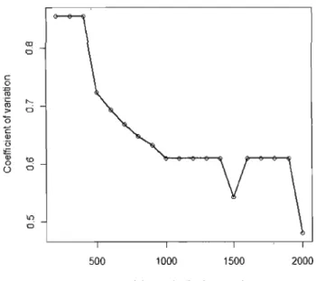
1.2. The mean coefficient of variation (CV) of the residence 26

1.3. Frequency of residence times computed 27

1.4. The use of agricultural1ands by Ring-billed Gulls 31

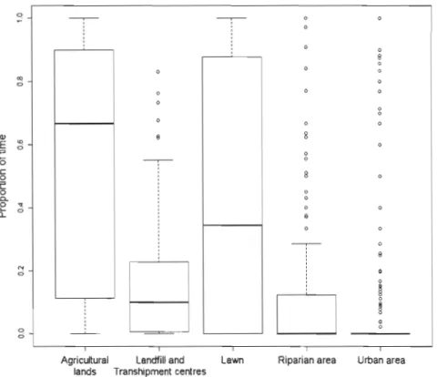
1.5. The proportion of time spent foraging by Ring-Billed Gulls 35

1.6. Diet of Ring-billed Gull chicks and breeding adults from the Deslauriers Island 36

LISTE DES TABLEAUX

Tableau Page

1.1. Coyer percentage of eight habitat types available in the foraging range 27 1.2. Sununary of a priori models considered to explain the probability that a Ring-billed Gull

will forage in a patch 28

1.3. Mixed-effects averaged logit RSF 29

1.4. Summary of a priori models considered to explain the risk that a Ring-billed Gullleave a

patch 32

1.5. Mixed-effects averaged COX model 33

1.6. Mean dry mass and mean energetic value of nine food items categories gathered in three

RÉSUMÉ

L'acquisition de nourriture est cruciale pendant la saison de reproduction des animaux, affectant particulièrement l'aptitude (jitness) de ceux qui rapportent de la nourriture à leur progéniture. Les oiseaux reproducteurs en quête alimentaire sont sownis à des contraintes inhérentes à leur état et à celui de leur progéniture, en plus des contraintes liées à la répartition spatiale et temporelle hétérogène des ressources et du risque de prédation. Ces contraintes mènent à des compromis impliquant l'énergie, le temps, la nutrition et le risque de prédation: il en résulte une séquence de localisations spatiales qui forment un déplacement. Mon objectif principal était de d'identifier la présence d'un tel compromis et d'identifier ses déterminants, à travers les déplacements de quête alimentaire du Goéland à bec cerclé (Larus delawarensis) durant la période de la nidification. On suggère souvent que

la densité élevée de goélands cause des problèmes en zones urbaines (e.g. propagation de micro-organismes pathogènes), mais le manque d'information sur son comportement empêche les autorités d'adopter des mesures de gestion éclairées. En 2009-2010, les déplacements quotidiens de 109 goélands adultes entre la colonie de nidification de l'île Deslauriers (Montréal) et les sites d'alimentation ont été enregistrés avec des consignateurs de localisations GPS de haute précision. De plus, le comportement alimentaire des adultes a été caractérisé par des observations hebdomadaires dans chaque type d'habitats. Des bols alimentaires de juvéniles et d'adultes ont aussi été récoltés. Pendant l'incubation, les goélands sélectionnaient fortement les terres agricoles de cultures annuelles où le travail de préparation des sols augmente la disponibilité d'annélides en surface. Les goélands sélectionnaient aussi les lieux d'enfouissement technique et les centre de transbordement où ils obtiennent non pas seulement une plus grande masse de nourriture, mais aussi une nourriture qui a un contenu énergétique moyen plus élevé que dans tout autre milieu. Par ailleurs, les contraintes de temps liées à l'incubation et à l'élevage semblaient inciter les goélands à éviter les milieux urbains où les opportunités d'alimentation sont très dispersées spatialement et temporellement.

INTRODUCTION

SÉLECTION D'HABITATS

Les besoins à combler par les animaux au cours de leur vie sont multiples: acquisition de nourriture, appariement pour la reproduction, défense contre les prédateurs, etc. Plusieurs choix s'offrent à eux pour répondre à ces besoins tels que choisir un site où se nourrir et quels aliments ingérer, choisir son partenaire et le moment de la reproduction. Ces choix s'expriment par des comportements limités par diverses contraintes (e.g. énergétiques, temporelles, physiologiques) issues entre autres des animaux eux-mêmes, de leur progéniture et des habitats disponibles. Tout comportement résulte d'un compromis reflétant ces diverses contraintes (Krebs et Davies, 1997). En écologie comportementale, le paradigme d'optimisation étudie les coûts et les bénéfices des comportements, en tant que réponses aux besoins des animaux. Il est possible de tester les avantages de différents compromis, et donc de différents comportements. Il s'agit de développer une fonction de l'aptitude (fitness), en liant une devise de l'aptitude à optimiser (e.g. gain énergétique, taux d'ingestion, etc.) aux contraintes imposées aux individus (Krebs et Davies, 1997).

Des concepts importants, comme la distribution libre et idéale (Fretwell et Lucas, 1969) et la théorie de la quête alimentaire depuis un point central (central-place foraging

theory; Orians et Pearson, 1979), ont été élaborés dans le cadre du paradigme d'optimisation

pour décrire les comportements optimaux dans l'acquisition de ressources alimentaires. Le gain net en énergie est une des devises d'aptitude couramment utilisées dans les modèles du paradigme d'optimisation, bien qu'étant seulement une mesure des bénéfices que l'individu retire à court terme de son comportement (Gaillard et al., 2010; Krebs et Davies, 1997). Par exemple, même si la valeur reproductive d'un individu est fonction de ses réserves nettes en énergie, le gain net en énergie d'un individu dans une parcelle ne nous informe pas directement de son succès reproducteur. La réserve nette en énergie est fonction du gain en énergie dans les parcelles visitées, des coûts en approvisionnement dans les parcelles et des coûts de déplacement à l'aller et au retour des parcelles (Olsson et al., 2008).

Les modèles de la distribution libre et idéale et de la théorie de la quête alimentaire depuis un point central sont généralement applicables à des expérimentations à très petites échelles. Ces dernières permettent souvent de négliger le déplacement et les contraintes qui y sont liées (coûts de déplacement, information incomplète sur la qualité des parcelles et information incomplète la présence de congénères aux parcelles; Bernstein et al. 1991; Beauchamp et al. 1997). Malgré des tentatives de prendre en compte le déplacement (Olsson

et al. 2008), ces modèles sont difficiles à appliquer par des expérimentations à l'échelle du

paysage. Le caractère incertain de l'information sur les parcelles ainsi que les capacités limitées de déplacement et de navigation ne peuvent pas être négligées (Lima et Zollner,

1996; Zollner et Lima, 1999; Nathan et al., 2008).

Alors que les modèles du paradigme d'optimisation ont surtout été étudiés par des expérimentations à fine échelle, d'autres modèles ont été développés pour décrire la sélection d'habitats par des animaux à l'échelle du paysage (Manly, 2002). Un habitat est défini conune un ensemble de variables biotiques et abiotiques distinct d'autres ensembles (Beyer et al.,

2010). Un habitat est sélectionné par un individu lorsqu'il est utilisé de manière disproportionnée par rapport à sa disponibilité qui est liée à son abondance et modifiée par son accessibilité (Buskirk et Millspaugh, 2006). La comparaison des habitats utilisés et des habitats disponibles permet d'établir des fonctions de sélection de ressources (fSR) (Manly, 2002). Diverses méthodes statistiques permettent à travers ces fonctions d'étudier la relation entre l'utilisation des habitats et leur disponibilité, en établissant le rôle de diverses covariab1es environnementales dans le processus de sélection (Manly, 2002). Toutefois, l'élaboration de fSR pose plusieurs clifficultés. On doit a priori définir arbitrairement la disponibilité des habitats pour la population animale étudiée, en supposant que l'animal est un organisme omniscient qui connaît parfaitement la disponibilité des ressources sur son territoire (Lima et Zollner, 1996). Il faut souligner qu'une variation de la disponibilité peut faire varier grandement les résultats des analyses de sélection d'habitats (Mysterud et Ims, 1998, Beyer et al., 2010). De plus, la plupart des fSR ne considèrent pas la variation d'accessibilité des habitats: la supposition est faite que tous les habitats dans l'aire d'étude sont également accessibles (Beyer et al., 2010; Gaillard et al., 2010). Déterminer adéquatement l'utilisation des habitats n'est pas non plus sans difficultés: c'est souvent

5

l'occupation (présence ou absence) gui est notée, sans discriminer le comportement des individus à chaque localisation spatiale (Barraquand et Benhamou, 2008; Beyer et al., 2010).

Par exemple, en étudiant la sélection d'habitats d'alimentation, les habitats utilisés sont ceux où les individus s'attardent pour leur recherche alimentaire, ingestion d'aliments, etc. Les habitats utilisés à d'autres fins ne devraient pas être classés comme des habitats utilisés pour l'alimentation.

ÉCOLOGIE DU DÉPLACEMENT

Malgré la limite de portée de certaines analyses, le nombre d'études publiées sur le déplacement animal est en constante augmentation (Holyoak et al., 2008). Toutefois, au-delà

des considérations méthodologiques, la majorité de ces études décrivent seulement l'occurrence du déplacement ou Les facteurs environnementaux qui influencent son occurrence. Peu d'études se sont intéressées à expliquer les déplacements de quête alimentaire tout en les liant aux besoins et aux oontraintes des animaux en déplacement (Holyoak et al.,

2008; Owen-Smith et al., 2010). Pour concilier l'écologie comportementale et l'écologie du

paysage, plusieurs auteurs ont souligné le besoin d'utiliser de nouvelles approches en se basant sur le développement rapide des méthodes de télémétrie et des systèmes d'information géographique (Shick et al., 2008; Cagnacci et al., 2010). Nathan et al. (2008) stipulent que la

localisation géographique, composante élémentaire du déplacement, résulte d'un compromis issu des contraintes intrinsèques à l'individu (état physiologique, capacités de déplacement et de navigation) et de contraintes externes liées à l'environnement biotique et abiotique. Dans le cadre du paradigme d'optimisation, le déplacement est un comportement ayant des coûts et bénéfices, surtout à l'échelle du paysage où les ressources ont une répartition spatiale particulièrement hétérogène. L'estimation des coûts et bénéfices, et ultimement l'estimation des performances individuelles et de l'aptitude, est difficile à mesurer. Toutefois, l'évolution de la technologie dans le domaine de l'écologie spatiale a permis le développement de nouvelles approches analytiques pour dépasser la simple documentation de l'occurrence du déplacement. Elles ouvrent progressivement la voie vers la quantification des impacts du déplacement sur les performances individuelles (Gaillard et al., 2010).

COMPLÉMENTARITÉS DES APPROCHES ANALYTIQUES

Pour pallier aux limites des FSR et faire le pont avec l'écologie comportementale, Fauchald et Tveraa (2003) ont proposé d'inférer la sélection d'habitats à partir de l'intensité d'utilisation des sites fréquentés par les animaux. Pour estimer l'intensité d'utilisation, ils utilisent le temps de résidence des individus à travers le paysage, ce qui peut être calculé de différentes façons (Johnson et a!., 1992; Barraquand et Benhamou, 2008). Dans tous les cas, le temps de

résidence varie selon le comportement des animaux, lesquels alternent généralement en.tre déplacements rapides et aires restreintes de recherche où ils réduisent leur vitesse et augmentent le nombre de virages (area-restricted search, ARS; Kareiva et Odell, 1987).

Ainsi, le temps de résidence peut servir à discriminer les localisations où les individus sont en recherche intensive de nourriture des localisations où ils sont en déplacement. Il s'agit de fixer un seuil de temps en se basant sur des considérations biologiques de l'espèce étudiée. Avec des données de présence seulement, issues par exemple de la télémétrie GPS, la comparaison entre les localisations de recherche alimentaire et les localisations de déplacement permet d'établir une FSR à partir du paysage expérimenté par les individus (Freitas et al., 2008). On peut ainsi surpasser deux difficultés des FSR classiques: la

définition subjective de I~. disponibilité des habitats et l'absence de discrimination entre l'utilisation d'un habitat et la simple occurrence.

Des analyses complémentaires peuvent aussi minimiser les mauvaises interprétations des FSR (Bastille-Rousseau et al., 2010). Selon certains modèles classiques du paradigme

d'optimisation, le temps de résidence dans une parcelle devrait diminuer avec la qualité de la parcelle et augmenter avec sa distance à partir d'un point central (Stephens and Krebs 1986). Ces suppositions doivent être nuancées. Un individu peut quitter une parcelle après satiation, avant l'épuisement de la ressource dans la parcelle (Iwasa et a!., 1981; Bastille-Rouseau, et al., 20 Il). Le temps de résidence peut aussi être influencé par la stratégie de recherche

alim nt ire dans chaque habitat. Par conséquent, la collecte de données sur les comportements aux sites d'alimentation, sur la qualité des parcelles et sur les facteurs individuels devient nécessaire à l'interprétation d'une analyse de sélection d'habitats (Owen­ Smith et al., 2010). L'analyse de la variation du temps de résidence peut aussi apporter une

7

information supplémentaire sur la qualité des habitats et le comportement des individus dans ces habitats: un individu peut effectuer le même nombre d'arrêts dans deux habitats différents, mais demeurer systématiquement plus de temps dans un des deux habitats. À ce titre, la combinaison de FSR, d'une analyse du temps de résidence et d'inventaires sur le terrain devrait fournir une bonne base pour l'étude de la quête alimentaire optimale et la sélection d'habitat à l'échelle du paysage.

POPULATIONS DE LARIDÉS

Au cours du dernier siècle, plusieurs populations de Laridés ont connu une croissance rapide partout à travers le monde. L'augmentation de la disponibilité des sites de nidification (baisse du niveau de l'eau et la création d'îles artificielles) et la multiplication des sources de nourriture anthropiques (lieux d'enfouissement technique (LET), terres agricoles et casse­ croûtes en milieu urbain) seraient largement à l'origine de la croissance des populations nicheuses (Conover, 1983; Pons, 1992; Duhem et al., 2008). La croissance de la population nord-américaine de Goélands à bec cerclé (Larus delawarensis) représente bien ce phénomène. En effet, les populations de Goélands à bec cerclé de l'Amérique du Nord étaient en déclin au début du XX· siècle à cause de l'exploitation de leurs plumes et de leurs oeufs et de la destruction de leurs sites de nidification (Ryder, 1993). La protection que la Convention concernant les oiseaux migrateurs leur a accordée à partir de 1916 a freiné ce déclin. Après l'établissement des premiers couples nicheurs de Goélands à bec cerclé dans la région montréalaise en 1953, la population nichant sur des îles du fleuve Saint-Laurent s'est accrue de manière exponentielle dans les années 1970 et 1980 (Mousseau, 1984) (Fig. 1). La population de' Goéland à bec cerclé de la région montréalaise qui se répartit en plusieurs colonies est maintenant jugée stable (Pierre Brousseau, comm. pers.). La plus grande colonie, celle de l'île Deslauriers à ['est de Montréal, accueillait 49000 couples nicheurs en 2009 (Pierre Brousseau, comm. pers.).

100000 80000 <il -0 S '0<li 60000 ­

'"

~ "_::; Ô :JOOOO Z 20000 _.

Ji

() 1976 1979 1982 1085 1988 1991 1994 1997 ~OOO ~003 2006 ~O()9

Figure 1. Nombre de nids de Goéland à bec cerclé dans la région de Montréal, 1978-2009. (Pie,rre Brousseau, SCF, données non publiées).

NUISANCES ATTRlBUÉES AUX LARIDÉS

La forte densité de goélands en milieu péri-urbain entraîne sa part de problèmes en zone urbaine. Dans un contexte de quête alimentaire depuis un point central, les goélands survolent fréquemment les installations humaines lors de leurs nombreux allers-retours entre la colonie et leurs sites d'alimentation. Les sources de conflits entres les goélands et les humains sont multiples. La première préoccupation des citoyens a trait à la propagation d'organismes pathogènes par les goélands (Moreau, 2012). En effet, les goélands sont porteurs de plusieurs types de bactéries qui peuvent être propagées par leurs fientes (Lévesque et al, 2000). Bien que les risques de transmission de pathogènes du goéland à l'homme sont minimes, il n'est pas totalement exclu qu'une contamination se produise sur les sites de baignade (Soller et al.,

20 l 0; Schoen et Ashboit, 20 l 0). Une autre préoccupation des citoyens sont les dommages causés aux infrastructures humaines par les fientes. Quoiqu'il soit difficile d'évaluer l'impact des fientes que les oiseaux laissent tomber en vol sur les habitations et les infrastructures des zones résidentielles, les dommages causés par les goélands nichant sur les toitures ont toutefois pu être quantifiés. En plus d'engendrer des désagréments aux employés d'entretien, les goélands produisent des fientes qui corrodent les revêtements et obstruent les drains. Vermeer et al. (1988) ont évalué que la présence de goélands nicheurs sur un bâtiment peut réduire de moitié la durée de vie de la toiture. Les goélands représentent aussi un risque de

9

collision important pour l'aviation civile (Dolbeer et al., 2000). De fait, Cleary et al. (1997) ont estimé que les goélands étaient responsables de 16% des collisions avec des aéronefs aux États-Unis alors que Belant (1997) a estimé les coûts annuels engendrés par ces collisions à 40 M$. Toutefois, la plupart de ces problématiques environnementales et de santé publique demeurent peu documentées, et donc hypothétiques. Les municipalités et les agences responsables reçoivent des plaintes, mais se voient impuissantes devant le manque d'information sur le comportement et la dynamique des populations de goélands. Par conséquent, elles ne peuvent pas agir efficacement dans la gestion des populations de goélands, dont celles du Goéland à bec cerclé qui sont souvent jugées surabondantes et nuisibles.

Le comportement alimentaire des goélands ayant une influence importante sur leur succès reproducteur (Annet1 et Pierotti, 1999), il s'ensuit que sa caractérisation serait primordiale pour mieux comprendre la dynamique des populations de Goélands à bec cerclé et gérer ces dernières, le cas échéant. De plus, les trajets que les goélands effectuent entre la colonie et les sites d'alimentation pour acquérir leur nourriture et celle de leurs jeunes ne sont pas connus. Une meilleure connaissance du comportement d'alimentation des goélands permettrait de mieux comprendre les facteurs déterminant la présence des goélands dans différents milieux et leur diète.

Les Goélands à bec cerclé sont considérés des généralistes au nIveau de leur alimentation (Ryder, 1993). Dans la région montréalaise, ils sont souvent observés cherchant de la nourriture tant dans les LET que dans les autres milieux urbains, les terres agricoles et en milieux naturels. Il faut toutefois noter que les LET sont maintenant sujets à des mesures de gestion qui visent à diminuer la disponibilité de nourriture aux animaux (zone active d'enfouissement des déchets réduite, recouvrement rapide des déchets et programmes d'effarouchement). Jusqu'à maintenant, le régime alimentaire de cette espèce n'a été étudié que pour les juvéniles nourris par les parents (Lagrenade et Mousseau, 1981; Brousseau et al, 1996). L'alimentation des adultes est méconnue dans l'aire d'étude, bien que le régime alimentaire des jeunes au nid semble être similaire à celui des adultes qui les nourrissent (Brown et Ewins, 1995). On ne cormaît pas plus l'importance relative des sites d'alimentation

dans le bilan énergétique des goélands. Si les sources anthropiques de nourriture représentent une fraction importante de l'alimentation des goélands en telmes de gain d'énergie net, des mesures prises pour diminuer l'accessibilité à ces sources de nourriture pourraient pelmettre le contrôle des populations.

Si l'avènement des suivis par système de positionnement GPS et le développement de nouveaux outils d'analyse ont engendré la multiplication d'études portant sur le déplacement des animaux (Holyoak et al., 2008), l'imprécision des localisations obtenues, leur faible fréquence et un nombre non négligeable de localisations manquantes ont souvent limité la portée de ces études (Frair et al., 2010). L'utilisation d'appareils fiables, précis (± quelques mètres) et à haute fréquence d'acquisition de localisations (intervalles en secondes ou minutes) rend maintenant possible l'étude de la sélection d'habitats d'alimentation par une espèce d'oiseau de taille moyenne comme le Goéland à bec cerclé (ca. 500 g) et qui s'approvisionne sur une échelle spatiale de quelques dizaines de kilomètres (Belant et al.,

1998).

Mon objectif principal était de documenter le processus d'utilisation d'habitat dans la perspective d'un compromis énergétique dans les déplacements de quête alimentaire du Goéland à bec cerclé, durant la période cruciale de la nidification. Pour ce faire, j'ai combiné une fonction de sélection de ressources et une analyse de temps de résidence basées sur un suivi télémétrique détaillé à des données d'inventaires, de régime alimentaire et d'analyses calorimétriques.

CHAPITRE 1 - FORAGING :\10VEMENTS OF BREEDING RING-BILLED GULLS IN A HETEROGENEOUS LANDSCAPE: WHICH HABITAT IS THE BEST?

SUMMARY

1. Foraging birds face several constraints that stem from their own and their offspring state as weil as from the heterogeneous distribution of food resources and predation risk that both vary in space and time. These constraints likely shape trade-offs involving time, energy, nutrition, and predation risk, leading to a sequence of spatial locations visited by foraging birds. However, few studies have addressed the deterrninants offoraging movements at the landscape level.

2. Here, we document tbe processes leading to habitat use by foraging Ring-billed Gulls

(Larus delawarensis) nesting in a large coloriy in suburban area using fine-scale

movement data collected by GPS (n = 109 birds) as well as in situ gull surveys and

gut content analyses.

3. Resource selection functions and residence time analyses showed that, during incubation, gulls prirnarily selected intensively cultured lands, which are doser to the colony but provided an intermediate mean energy intake based on calorimetrie analyses. According to ground surveys, gull abundance in agricultural lands was greater on bare soil and increased during periods of soil preparation and seed sowing.

4. According to the models, gulls strongly selected landfills and transhipment centres throughout the breeding season as these sites provided the highest mean energy intake. Nevertheless, only few individuals highly selected these localised and limited sites. Distance to the colony and the deterrence programs conducted at sorne landfills probably increased foraging costs.

5. Our approach based on a combination of methods and derived from an energetic trade-off perspective offers a framework to understand animal foraging movements. Combined with data on individual breeding performance, this could provide relevant information on the rnid-term benefits of habitat choice.

1.1 INTRODUCTION

During the breeding season, most animais must find food as weil as attend and rear their offspring while avoiding predation. Animais must thus face time and energy constraints leading to trade-offs in their activity budget. Optimal foraging theory specifically dwells on these trade-offs for resource acquisition (Stephens and Krebs, 1986; Giraldeau and Caraco, 2000). Traditionally, models such as the marginal-value theorem and ideal free distribution have been used to assess the trade-offs of where and when animais should feed (Fretwell and Lucas, 1969; Orians and Pearson, 1979). These models, however, are usually applied to small scale systems while assuming that animais incur low travel costs and are highly infonned about their enviroÎunent (Stephens and Krebs, 1986; Giraldeau and Caraco, 2000). Consequently, these models are more difficult to apply at the landscape level where infonnation uncertainty about the environment as weil as the limited motion and navigation capacity of animais carmot be neglecled (Lima and Zollner, 1996; Nathan et a!., 2008).

Following Lima and Zollner (1996), many authors have called for new approaches to bridge the gap between behavioural and landscape ecology. The fast and recent development of wildlife telemetry and geographic information systems (GIS) has opened one such avenue (Shick et al., 2008; Cagnacci et al., 2010). As underlined by the conceptual framework of

movement ecology proposed by Nathan et al. (2008), a movement path is the result of a

complex interaction between factors that are internai (physiological state, motion and navigation capacity) and external to the individuals (abiotic and biotic environments). Within the optimality paradigm, a movemeot path would accordingly be the outcome of balancing trade-offs subject to sorne constraints in the acquisition of resources, especially within a landscape where resources are heterogeneously distributed. Although assessing the costs and benefits of large scale movements is difficult, new analytical methods based on accurate location data (e.g., GPS) are now available to study movement behaviour and its associated cost-benefit trade-offs (Gaillard et al., 2010).

Resource selection function (RSF) is one of the classical approaches used by landscape ecologists to assess habitat use. It is based on the comparison of habitat use and availability using presence-only or presence/absence of individuals in habitat patches (Manly

et al., 2002). Use locations and their associated habitat characteristics are noted at different

time intervals, while available habitats are often simply defined as the habitats mapped within the estimated home range (Johnson, 1980; Manly et al., 2002). This definition of availability

is based on the assumption that ail habitats within the home range are equally accessible, ignoring that habitat availability results from both abundance and accessibility (Buskirk and Millspaugh, 2006). Furthermore, it assumes that habitats outside home range boundaries are not accessible. This is a pervasive problem with telemetry data because home ranges are deterrnined with presence-only data (Amis et al., 2008). Another critique concerns the lack of

discrimination among locations according to the intensity of use and the activity performed at the locations (Freitas et al., 2008; Beyer et al., 2010). RSFs wou Id definitely be more

informative if they could distinguish between actively se1ected locations (e.g., foraging patches) and the incidentally selected locations (e.g., interpatch movements) (Barraquand and Benhamou, 2008; Beyer et al., 2010).

In the case of presence-only data, the difficulty of defining available habitats can be avoided by building RSFs from visited habitats only (Freitas et al., 2008). Indeed, the

comparison between locations occurring in foraging patches and during interpatch movements can reveal how habitats are selected (Freitas et al., 2008). Considering the

heterogeneous spatial distribution of resources, animais should increase their search effort in areas characterized by high resource density and thus adopt a movement pattern named area­ restricted search (ARS). Individuals shou1d accordingly reduce their speed and increase their

turning rate, thereby increasing the time spent in the area (Kareiva and Odell, 1987; Benhamou, 1992). Therefore, considering the time spent within the surroundings of recorded locations (residence time) should help discriminate between locations comprised within foraging patches and those part of interpatch movements (Fauchald and Tveraa, 2003; BalTaquand and Benhamou, 2008). Based on biologically relevant considerations, a time thresbold can be fixed to discrirninate between foraging patch and interpatch movement locations.

15

To minimize the risk of misinterpreting a fitted RSF, Bastille-Rousseau et al., (2010) recommended that complemeIltary analyses be used. For instance, the analysis of residence time as an index of the intensity of use could provide valuable information on both patch quality and behaviour of the animal at specifie patches. According to classical optimal foraging models, the time spent in a patch should depend on patch quality and the distance among patches or between patches and a central-point (Stephens and Krebs, 1986). However, considering that consumers c~m use different patch departure rules (Bastille-Rousseau et al., 2011), the analysis of residence time should be combined with in situ observations documenting individual foraging strategies (activity budget), patch quality (rates of food intake, diet, energetic quality of food conswned), environrnental conditions (meteorological factors) and individual characteristics (sex, age, physiological condition, breeding phase) (Owen-Smith et al., 2010). A. combination of RSF, residence time analysis, and in situ surveys should thus provide sorne insight into the study of optimal foraging and habitat selection at the landscape level (Bastille-Rousseau et al., 2010).

Accordingly, we used RSF and residence time analyses from GPS-tracking data, as wel1 as in situ surveys, diet characterization, and calorimetrie analyses to address the processes that determine the habitat use of breeding Ring-billed Gulls (Larus delawarensis) from an energetic trade-off perspective. As observed worldwide for numerous gull populations, the number of IUng-billed Gulls has increased dramatically in the last 30-40 years (Conover, 1983; Smith and Carlile, 1992; Duhem et al., 2008). These demographic increases have been largely associated to a greater availability of anthropic food sources such as landfills, garbage mismanagement, food handouts, intensively managed agriculturallands, etc. (Pons, 1992; Belant et al., 1997). The strong nwnerical response of Ring-billed Gulls in face of this anthropic food 1S not surprising given that these colonial central-place foragers already fed opportunistically upon a wide diversity of prey items found in different habitats (Ryder, 1993; Brousseau el al., 1996). These characteristics along with its high abundance

and large body size make the Ring-billed Gull an interesting model to document the process leading to habitat use by foraging birds in a heterogeneous landscape, particularly during the crucial breeding period.

1.2 METHüDS

1.2.1 STUDY AREA

We tracked the movements of Ring-billed Gulls across the Montreal metropolitan cornmunity (CMM), Quebec, Canada, in 2009-2010. This area covers 4360 km2 and was then home to ca. 3.7 million people distributed among 82 municipalities. Land use included farmlands (51%), urban areas (37%), and waterways (12%). About 70,000 pairs of Ring-billed Gulls nested in 4 colonies within the CMM. We limited our observations to birds breeding in the largest colony (48,000 pairs), which is located on Deslauriers Island (45.717°N, 73A33°W;

Canadian Wildlife Service, unpublished data). The island spans lIA ha and is located 3 km downstream from the island of Montreal in the St. Lawrence River.

The CMM consists of a mosaic of high and low density urban areas, agricultural lands of intensive (soybean, maize, and small cereals) and extensive cultures (hayfields and pastures), as weil as riparian habitats along the St. Lawrence River and its tributaries (Fig. 2). Four landfills and two open transhipment centres were located in the vicinity of the colony. During our study, the Saint-Thomas and Lachute landfills located at 41 and 63 km from the colony, respectively, had no deterrence program. The Ste-Sophie landfill (37 km) initiated a deterrence program in 2009 which combined pyrotechnics and rifle shooting; the program was limited to weekdays from 07:00 to 15:00, providing sorne windows of feeding opportunities. The Lachenaie landfill (8 km) had a deterrence program since 1995 that include falconry, distress calls, and pyrotechnics; this program was in operation every day from sunrise to sunset, preventing all but few gulls to access and use the landfill (Thiériot, 2012). The two transhipment sites located at 12 and 27 km from the Deslauriers Island colony, respectively, ran no deterrence program.

o

10 20 Kilometers 1 1 1 1 1 Figure 1. Study area. Land cover types include waler (white), urban areas (Iight gray), agricultural lands (dark gray) and forest (black). Open squares indicate landfills locations (L-Lachute, 2-St~Sohpie, 3-Lachenaie, 4-Saint-Thomas), open triangLes indicate transhipment centres locations, and open circ!es indicate Des Lauriers Island. ~ -..J

1.2.2 TELEMETRY

Breeding Ring-billed Gulls (n = 109) were fitted with 10-15-g GiPSy-2 data loggers (Technosmart, Italy) between mid-April and late June 2009-2010. Data loggers represented (mean ± SD) 2.8 ± 0.5% of the birds' body mass (485 ± 49 g). While gulls were captured and recaptured with nest traps during incubation (Verreault et al., 2004), gulls with chicks were

captured with a dip net near their nest and recaptured by rifle shooting in accordance to a Canadian Wildlife Service scientific permit (carcasses were kept for further analyses, see

Diet section). Data loggers were attached on the two median rectrices with white TESA tape

(no. 4651) and programmed to acquire locations at 4-min interva1s for 1 to 3 days. Breeding stage was noted at capture distinguishing between the incubation period for a bird with a nest containing eggs, and the rearing period for those with at least one hatched egg. Methods were approved by the Institutional Animal Protection Committee of the Université du Québec à Montréal (No.646).

1.2.3 GULL SURVEYS

We ,conducted surveys in the main feeding habitats of Ring-billed Gulls to determine the proportion of time gulls spent foraging in each habitat type. Surveys were carried out weekly during the breeding period, altemating between three 5-h periods (5:00-10:00, 10:00-15:00, and 15:00-20:00) that covered the entire daylight. In agricultural habitats, we surveyed a 50­ lan roadside transect bordering each shore of the St. Lawrence River in 2009 (n = 13 surveys) and 2010 (n = 21 surveys). We tallied the number of birds composing each flock and performed an instantaneous scan sampling to deterrnine the proportion of birds foraging (head down below the horizontal or probing into the soil). We considered this value as the proportion of time spent foraging (Altmann, 1974). A flock was defined as a group of gulls using the same field type and not separated by more than 200 m from each other. Birds using different field types but c10ser than 200 m from each other were considered as being part of different flocks and were considered independent samples. The total number of tractors and their activity (ploughing/harrowing or sowing) were also noted over the entire transect during each survey, regardless the presence of gulls in the field.

19

Observations in other habitats were conducted weekly in 2010 along three fixed point transects crossing urban (n

=

25 points), suburban (n

=

53 points), and riparian (n

=

10 points) areas on the Montreal Island (n

=

16 surveys) and along the North (n

=

18 surveys) and the South shores (n = 22 surveys) of the St. Lawrence River. At each point, gulls using different habitat types (lawn; shore; grounds with concrete, asphalt or gravel; building roofs; and post lights) were counted and scanned to detennine the proportion of birds foraging (erratic flight in emergent insect clouds above waterbodies, feeding on garbage, head down below the horizontal or probing into the soil or water).

Finally, we estimated the proportion of time gulls spent foraging in landfills by conducting 5-h observation periods once a week in 2009 (n

=

7) and 5 days a we~k in 2010 (n = 59) at the Ste-Sophie landfill, again alternating among the 3 daily periods. Total bird counts and instantaneous scan sampling were conducted every half hour from a high point allowing observation of the entire site. The mean daily abundance of gulls was computed for each day as weil as the proportion of birds that were actually foraging (flying less than 5-m above the active tipping area, head down below the horizontal or probing into refuse).

1.2.4 DIET AND CALORlMETRlC ANALYSES

We collected boli from chicks of both sexes during weekly visits to the Deslauriers colony during the rearing period of 2009 and 2010. We selected chicks haphazardly and slightly pressed their proventriculus to make them regurgitate recently swallowed food. Spontaneous regurgitations of adults and juveniles captured during banding operations were also collected. Samples were stored in a cooler until they could be put in a freezer at the end of the day.

We also kept frozen the carcasses of adults fitted with data loggers and recaptured by shooting until their stomach content was analysed, separating material from the oesophagus and proventriculus. Similarly, we analysed stomach contents of birds collected by rifle shooting in agricultural lands (n

=

69), riparian areas (n

=

54), and at the Ste-Sophie landfill (n

=

85) in accordance with Canadian Wildlife Service scientific permits. For security reasons, gulls could not be collected in urban areas.

Each food item of a bolus or stomach was separated, identified, dried to constant weight (± 0.01 g), and weighted. Food items were grouped into broad categories (e.g., arthropods, annelids, vertebrates, refuse, vegetation, other). Although we measured both the volume and dry mass of food items, we only present results for dry mass as both measures gave consistent results and since dry mass was needed for calorimetrie analyses. We performed duplicate or triplicate calorimetrie analyses using a bomb calorimeter (parr, mode! 1108P) for each broad category of food items. Samples of each food category were pooled and ground before analysis.

1.3 DATA ANALYSIS

1.3.1 TELEMETRY

We first created a 300-m buffer zone around the Deslauriers Island to account for the lowering water levels during the surnmer which increase the island area and to discriminate between short movements to the shore or nearby shallow water where gulls rest or preen their feathers from foraging trips. Our analyses were limited to locations outside this zone. The mean number of foraging trips per day, the mean direct distance between the colony and the furthest location reached during a foraging trip (whether a stopover or not), the mean foraging trip traveled distance and the sinuosity (traveled distance divided by direct distance) were compared between breeding periods (i.e., incubation and rearing), using linear mixed models with gull ID treated as random factor. We then calculated the time spent by each gull at different locations on the landscape by estimating residence time without rediscretization (Barraquand and Benhamou 2008). Residence time was defined as the time spent in a circle of radius r centred at a given location along the foraging trip. The circle, with its specifie habitat composition and features, could then be viewed as a potential foraging patch. Because residence time is scale-dependent, the choice of the spatial scale, and thus the circle radius, is crucial (Lima and Zollner, 1996). Currently, there is no objective method to choose the appropriate scales given a specifie analysis or data set. Decisions must therefore be taken following data exploration and based on biological considerations (visual perception, resource density, etc.). Hence, for each path, we computed the coefficient of variation (CV)

21

of residence times measured for radii ranging from 200 to 2000 m using 100-m increments. We ignored radii sma11er than 200 m because we wanted to explore the relationship between habitat features and foraging movements at the landscape level. We then averaged the CVs measured with a given radius across paths and plotted the mean CVs of residence time against the circle radius. We considered that the highest CV should occur at the spatial scale that best contrasts "foraging patches" from areas characterized by transit movements. We fina11y retained locations distanced by at least 2 radii for the habitat use analysis to limit spatial autocorrelation (Fauchald and Tveera, 2003).

We created a land caver map of the study area in ArcGIS 9.3.1 (ESRl 2009) using both agricultural and topographie data (Base de dOMées des cultures assurées, La Financière agricole du Québec, 2009-201 0, planimetrie precision: < 4 m; CanVec, Natural Resources Canada, 2010, planimetrie precision: < 25 m; Land Coyer, Circa 2000 - Vector, Natural Resources Canada, 2009, planimetrie precision: < 30 m). We then calculated the landscape composition of each circle in which residence time was estimated. Landscape composition was defined as the proportion of different broad categories of habitats including lawns, woodlots, urban areas, water, intensive cultures, extensive cultures, and unidentified culture. Because of their relatively sma11 size, landfills and transhipment centres were noted as presence/absence in each circle. We also measured the distance between each location where a residence time was computed and the nest of the tracked gull. Fina11y, we calculated the mean daily rainfall for the CMM, using data from 10 meteorological stations located on both shores of the St. Lawrence River (Environment Canada, 2010).

1.3.2 RESOURCE SELECTION FUNCTION

We estimated a RSF to investigate the factors that lead a gu11 to forage in a patch instead of passing through it. We first determined the different habitats available to the birds breeding on Deslauriers Island by estimating the proportion of habitats (based on the categories described above) found within the 100% minimum convex polygon drawn using the foraging trip locations of a11 birds. CODsidering that a foraging individual must reduce its flying speed and increase its turning rate, we then used residence time to discriminate foraging patches

from movement patches. We assumed that if a gull spent more than 100 s in a 200-m radius circie, it was foraging. If it spent less than 100 s, we assumed that the bird was moving either between the colony and a foraging patch or between two foraging patches. The vast majority of gulls observed during surveys spent more than 100 s when foraging within a 200-m radius circie. Based on flight speed of Black-headed Gulls (Chroieocephalus ridibundus) and Lesser Black-backed Gulls (Laros fuse us) that are respectively slightly smaller and larger than Ring­ billed Gulls (14.7 - 15.5 m s-', respectively; Shamoun-Baranes and van Loon, 2006), at least 26 s is required to cross a circle of 200-m radius. The remaining 74 s appears insufficient for a gull to forage in such a circular patch.

We used mixed-effects logistic regressions to quantify the influence of landscape composition on the probability that a gull foraged in a patch. Gull ID and foraging path ID (nested within gull ID) were treated as random factors. The addition of these terms dealt with the hierarchical structure of the data and allowed the estimation of the variability observed across individuals and movement paths. Eight different models were built and compared based on the second-order Akaike information criterion (AIC" Burnham and Anderson, 2002). We inciuded the relative coyer of each habitat category (lawns, woodlots, urbanareas, water, intensive cultures, extensive cultures, and unidentified cultures) and the occurrence of landfills or transhipment centres in ail eight models. We considered the interaction of rainfall with lawns as weil as with each type of agricultural coyer because these habitats show high abundances of annelids under wet conditions (Sibly and McCleery, 1983). We also included the distance between the location of a gull while foraging and its nest as a proxy for foraging costs and accessibility (Matthiopoulos, 2003). We considered distance both as a simple effect and in interactions with the relative amount of each habitat type (except woodlots) as weil as with the occurrence of landfills or transhipment centres because we do not know which fitness currency the gulls may be maximizing and since the profitability of the different habitat may not scale l' early with di tance. Alth ugh wood lots are accessible to gulls, these birds avoid being under canopy and should thus avoid forest habitats whatever the distance from the colony. Finally, we included the breeding stage (incubation or rearing) in interaction with each habitat variable to investigate the difference in habitat use during these two periods. This allowed us to take into consideration the gulls' breeding phenology and their

23

associated requirements as weil as habitat phenology, particularly for agricultural cover types where farming practices and field conditions vary strongly during a season. We fitted the mixed-effects logistic regressions using the Laplace approximation within the package Ime4 version 0.999375-39 of the R software version 2.12.2 (Bates et al., 20 II; R Development

Core Team, 2011). AlCc was computed based on maximum log-likelihoods. Multimodel

inference was performed following Burnham and Anderson (2002). We report model­ averaged coefficients as weLl as their unconditional standard errors and 95% confidence intervals.

1.3.3 RESIDENCE TIME ANALYSlS

Following Freitas et al. (2008), we used mixed-effects Cox proportional hazards models

(CPH model, Cox 1972) to investigate the relationship between residence time and the spatial, environmental, and individual explanatory variables. As for the RSF, we treated gull ID and foraging path ID (nested within gull ID) as random factors to take into account the hierarchical structure of the data (Pankratz et al., 2005; Freitas et al., 2008).

We used and compared by AlCc the same eight models developed for the RSF

analyses described above to investigate the determinants of residence time. Ali variables of the candidate models satisfied the CPH model assumption of proportionality, which was verified by visual investigation of the scale based on Schoenfeld residuals and testing whether their slope was equal to zero. This was done using fixed-effects CPH models because this procedure is not yet implemented for mixed-effects models. We computed AlCc

using penalized log likelihood and penalized degrees of freedom (Pankratz et al., 2005;

Freitas et al., 2008.). The CPH models and their assumption verification were computed

using the Survival and Coxme packages in the R software (Themeau, 2011a; Themeau, 2011b). Multimodel inference was performed following Burnham and Anderson (2002). We report model-averaged coefficients as weil as their unconditional standard errors and 95% confidence intervals.

1.3.4 SURVEYS

We quantified variation in the proportion of time spent feeding among habitats usmg a generalized linear model with logit link function and binomial error distribution. The proportion of gulls (in a flock) observed foraging was considered the response variable while the habitat categories (lawns, urban areas, riparian areas, and agricultural lands) were the explanatory variables weighted by the total nwnber of gulls. We also explored whether the abundance of gulls in agricultural lands was related to the total nwnber of tractors encountered along. transects in that same habitat, which was considered an index of agricultural field work. A generalized linear model with log link function and Poisson error distribution was fitted with the abundance of gulls along each transect as response variable and three explanatory variables: the nwnber of tractors, the transect location (South shore or North shore) and the interaction between the two.

1.3.5 DIET & CALORIMETRY

We first computed the proportion of boH contaiIÙng each broad category of food items for both chicks and adults. We then calculated the mean relative amount of each broad categOl)l­ of food items when present based on dry mass. The energy value of boli in kilojoules was calculated for each gull collected at the Ste-Sophie landfill, in agricultural lands, and at riparian sites by combining the dry mass of the items found in the stomach and its energy value measured with the calorimetrie bomb. We finally compared the mean energy value of boli (kJ) across habitat categories using an Anova.

1.4 RESULTS

We recaptured 109 Ring-billed Gulls of both sexes with GPS data loggers that provided reliable data. After removing locations within the 300-m buffer zone around the colony, there were only 28 missing locations on a potential of 15,620. The remaining 15,592 locations had a low dilution of precision metric (DOP :::; 6) (Frair et al., 2010). A total of 67 gulls were

25

followed during the incubation period (173 foraging trips) and 42 during the rearing period (229 foraging trips).

1.4.1 CHARACTERlSTICS OF FORAGING TRIPS

The mean number of foraging trips per day was greater during the rearing period (3.1 ±

1.0 trips'dai') than during incubation (1.9 ± 0.8 trips'dai l; t

=

-7.01, df

=

107, P < 0.01). Furthermore, the mean direct distance between the colony and the furthest location reached during a foraging trip (whether a stopover or not) was also greater during the rearing period (16.6 ± 12.4 km, maximum 63.5 km) than during incubation (12.5 ± 9.9 km, maximum 42.4 km; t = - 2.22, df= 107, P > 0.01). The mean foraging trip traveled distance was lower during incubation (30.2 ± 23.8 km, maximum 104.7 km) than during the rearing period (38.6 ± 29.0 km, maximum 155.9 km; t = -2.55, df= 107, P = 0.01), but no difference was found between the sinuosity index (traveled distance divided by direct distance) calculated during incubation (2.4 ± 0.40, maximum 5.0) aud rearing periods (2.3 ± 0.4, maximum 5.8; t = 1.38, df = 107, P

= 0.17).

1.4.2 SELECTION OF A SPATIAL SCALE

We observed a plateau of the mean CV s of residence time across paths for radii varying between 200 and 400 m ratller than a c1ear peak (Fig. 3). We tbus chose to use the 200-m radius for our analyses to ge1 a stronger contrast between the habitat composition of foraging and movement patches. Nevertbeless, we also conducted the analyses using a 400-m radius (the largest radius showing a high coefficient of variation of residence time) and reached the same conclusions as with the 200-m radius.

ID a c 0 ro "" .~ 1'-, a

'"

'0 C Cl <; iE Cl ID 0 _a U 500 1000 1500 2000

Spatial scale (radius in melers)

Figure 2. Mean coefficient of vanatlOn (CV) of

residence times of breeding Ring-billed Gulls within circular patches of different radii and centred on locations obtained by GPS data loggers (n = 109).

1.4.3 RESOURCE SELECTION FUNCTION

The composition of foraging and movement patches was highly variable (Table 1). Nevertheless, woodlots, intensive and extensive cultures represented a smaller percentage of both movement and foraging patches when compared to the whole foraging range. An opposite trend was found for urban areas, water bodies, landfills and transhipmentcentres. While woodlots and urban areas covered a smaller proportion of foraging patches than movement patches, intensive cultures were relatively more important in foraging patches. Landfills and transhipment centres had also a

27

Table 1. Cover percentage of eight habitat types available in the foraging range of 109 Ring­ billed Gulls nesting on Oeslauriers island and mean cover percentage (± SO) in movement (residence time < 100 s) and foraging (residence time ~ 100 s) patches, 2009-2010.

Habitat type Cover %

Home range Movement patches Foraging patches

(5565 km2 ) (n=2599) (n= 4490)

Lawns (parks, golf courses, etc.) 1.2 1.8 ± 8.3 2.1±9.4

Wood lots 20.6 13.7 ± 28.8 4.8 ± 16.0 Urban areas ]6.8 27.8 ± 38.5 23.1 ± 36.6 Waterbodies 5.3 18.7 ± 34.8 22.4 ± 37.9 Intensive cultures 39.5 24.3 ± 34.1 31.4 ± 38.7 Extensive cultures 11.7 8.4± 16.2 8.0 ± 15.6 Unidentified cultures 4.1 3.4 ± 12.3 4.2 ± 14.3 Landfills/Transhipment centres 0.1 1.3 ± 11.3" 4.2 ± 20.0" " Percent of occurrence 0 0 N ~ 0 0 0 ~ 0 0 a> ,., ü c: Q) ₀ :> 0 ~ <0 L"­ 0 0 '1' 0 0 N 0

r---r---.---.-I!

~I

0 500 1000 1500 19500 Residence lime (5)

Figure 3. Frequency distribution of residence times of breeding Ring­ billed Gulls within 200-m radius circular patches centred on locations obtained by GPS data loggers (n = 109).

higher percentage of occurrence in foraging patches compared to movement ones. The distribution of residence time was strongly skewed to the right, peaking below 100 sand reaching values up to 19,377 s (Fig. 4).

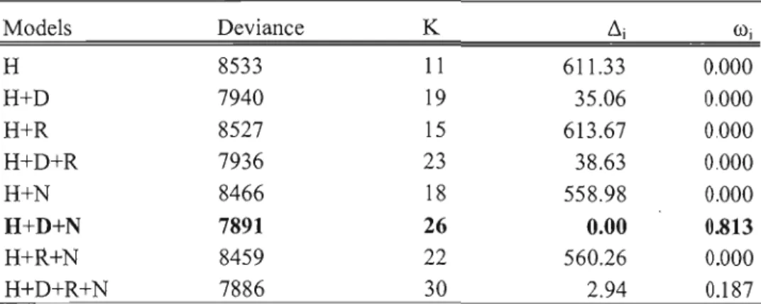
The best mode! (w; = 0.813) included habitat variables as well as variables characterizing the distance separating the patch from the colony and the breeding stage (Table 2). The model with rainfall scored as the second best mode! (w; = 0.187, Table 3). The same two models were selected for other time thresholds (60, 80, 120, and 140 s) with radii of 200 and 400 m (results not shown).

Table 2. SU111ll1,ary of a priori models (resource selection functions) considered to explain the probability that a nesting Ring-billed Gull will forage in a patch (H, habitat types; D, distance between each location and the colony; R, the mean dai1y rainfall within the foraging range; B, the breeding stage [incubation or rearing]), deviance, number of parameters (K), !li, Akaike weight (üli) for 100-s residence time threshold.

Mode1s Deviance K !li üli

H

8533 Il 611.33 0.000

H+D

7940 19 35.06 0.000

H+R

8527 15 613.67 0.000

H+D+R

7936 23 38.63 0.000

H+N

8466 18 558.98 0.000

H+D+N

7891 26 0.00 0.813

H+R+N

8459 22 560.26 0.000

H+D+R+N

7886 30 2.94 0.187

Ring-billed Gulls had a greater probability of foraging in a patch that was located further from the colony (Table 3). The probability also increased with the proportion of intensive cultures found in a patch during the incubation period. This period extended from mid April to mid-May when the presence of gulls in intensive agricultural lands was related to field work such as ploughing, harrowing, and sowing (Fig. 5). Accordingly, the number of gulls observed along transects in agricultural lands increased with the number of field

29

working tractors (jJ ± SE = 0.064 ± 0.001, Z = 53.9, P < 0.01). Of 20,900 gulls counted along

these transects, 52% were observed on bare soil fields, 34% on fields with low height

Table 3. Mixed-effects averaged logit resource selection functions (Table 2) quantifying the probability that a nesting Ring-billed Gull forage in a patch. Parameter estimates (~), unconditional standard errors (SE), and 95% confidence interva1s (CI) are presented.

Variable

p

SE 95 %CI Intercept -0.612 0.491 -1.575 0.351 Distance (km) 0.089 0.013 0.063 0.115 Woodlot -2.963 0.448 -3.840 -2.086 Lawns -0.212 0.834 -1'.846 1.422 Urban areas -2.550 0.521 -3.570 -1.529 Landfill 0.992 0.510 -0.007 1.992 Water -1.130 0.516 -2.142 -0.118 Extensive cultures -1.037 0.619 -2.251 0.177 Intensive cultures -0.901 0.516 -1.913 0.111 Unknown cultures -0.319 0.688 -1.666 1.029 Lawns X Distance 0.017 0.033 -0.049 0.083

Urban areas X Distance 0.067 0.016 0.036 0.098

Landfill X Distance 0.001 0.017 -0.033 0.035

Water X Distance 0.031 0.016 -0.001 0.063

Extensive cultures X Distance -0.005 0.021 -0.045 0.035 Intensive cultures X Distance -0.026 0.015 -0.056 0.004

Unknown cultures X Distance -0.036 0.026 -0.087 0.015

Lawns X Incubation -0.050 0.671 -1.365 1.266

Urban areas X Incubation 0.210 0.244 -0.267 0.688

Landfill X Incubation 0.271 0.446 -0.603 1.145

Water X Incubation 0.205 0.254 -0.294 0.703

Extensive cultures X Incubation -0.349 0.418 -1.168 0.469

Intensive cultures X Incubation 1.429 0.237 0.965 1.893

Unknown cultures X Incubation 0.911 0.474 -0.018 1.839

Lawns X Rainfall 0.038 0.019 0.001 0.075

Extensive cultures X Rainfall 0.000 0.007 -0.013 0.013 Intensive cultures X Rainfall -0.002 0.004 -0.009 0.005 Unknown culturess X Rainfall -0.003 0.008 -0.019 0.012

vegetation, 8% on stubble fields and the remaining 6% on mowed fields.

Gulls had a strong tendency to forage in a patch where a landfill or transhipment centre was present (Table 3). Gulls also foraged in patch with lawns during rainy days. On the other hand, gulls avoided foraging in a patch that included a high percentage of woodlots. The probability that gulls foraged in a patch also decreased with the relative cover of urban areas, but this effect was reduced as the gulls moved further from the colony.

Multimodel inference performed with time thresholds other than 100 s lead to model­ averaged coefficients highly similar to the ones presented in Table 3. Furthermore, the presence of a landfill or transhipment centre increased significantly the probability of foraging in a patch when a threshold of 60, 120 or 140 s was used to distinguish foraging patches from interpatch movements. Only for the 80-s threshold that there was no clear trend concerning the effect of landfilVtranshipment centre in the RSFs.