Optimization of a landfill gas collection shutdown based on an adapted first-order decay model

1 of 30

Optimization of a Landfill Gas Collection

Shutdown Based on an Adapted First-Order

Decay Model

Daniel A. Lagosa_{, Martin Héroux}b_{, Ryan Gosselin}c _{and Alexandre R. Cabral}d,*

1

a_{Engineer, Biothermica Technologies Inc., Montreal, QC, Canada. Formerly with}

2

Centre Universitaire de Formation en Environnement (CUFE), Université de

3

Sherbrooke, Sherbrooke, QC, Canada . daniel.lagos@usherbrooke.ca

4

b _{Engineer, City of Montreal, Montreal, QC, Canada. mheroux@ville.montreal.qc.ca}

5

c _{Associate Professor, Department of Chemical Engineering, Université de Sherbrooke,}

6

Sherbrooke, QC, Canada J1K 2R1. ryan.gosselin@usherbrooke.ca

7

d _{Professor, Department of Civil Engineering, Université de Sherbrooke, Sherbrooke,}

8 QC, Canada J1K 2R1. alexandre.cabral@usherbrooke.ca 9 10 *_{Corresponding Author} 11 12

Lagos, D.A., Héroux, M.#, Gosselin, R. and Cabral, A.R. (2017). Optimization of a landfill gas collection shutdown based on an adapted first-order decay model. Waste Management, 63: 238-245. http://

2 of 30

ABSTRACT

13

LandGEM’s equation was reformulated to include two types of refuse, fast decaying refuse 14

(FDR) and slow decaying refuse (SDR), whose fractions and key modeling parameters k 15

and L0 were optimized independently for three periods in the life of the Montreal-CESM

16

landfill. Three scenarios were analyzed and compared to actual biogas collection data: 1) 17

Two-Variable Scenario, where k and L0 were optimized for a single type of refuse; 2)

Six-18

Variable Scenario, where three sets of k and L0 were optimized for the three periods and

19

for a single type of refuse; and 3) Seven-Variable Scenario, whereby optimization was 20

performed for two sets of k and L0, one associated with FDR and the second with SDR, and

21

for the fraction of FDR during each of the three periods. Results showed that the lowest 22

error from the error minimization technique was obtained with the Six-Variable Scenario. 23

However, this scenario’s estimation of gas generation was found to be rather unlikely. The 24

Seven-Variable Scenario, which allowed for considerations about changes in landfilling 25

trends, offered a more reliable prediction tool for landfill gas generation and optimal 26

shutdown time of the biogas collection system, when the minimum technological threshold 27

would be attained. The methodology could potentially be applied mutatis mutandis to other 28

landfills, by considering their specific waste disposal and gas collection histories. 29

30

KEYWORDS: Landfill gas collection; First-order decay model; LandGEM; IPCC

31

model; Fast-decaying refuse; Slow-decaying refuse 32

3 of 30

INTRODUCTION

34

When landfill methane (CH4) generation reaches a critical low value, the system employed 35

to burn biogas must be replaced or, conditions permitting, shut down. The decision-making 36

process is challenging because of the difficulty in predicting relatively accurate future 37

trends sufficiently in advance. This is the type of challenge being faced by the operator of 38

the Montreal CESM landfill. This 72-ha site, which accepted refuse from 1968 to 2008, is 39

located in a former limestone quarry, in a (now) densely populated area of Montreal. The 40

depth of refuse reaches 80 m in certain areas, and it is estimated that some 40 million tons 41

of refuse from various origins were landfilled at the CESM landfill site. Prior to the 42

beginning of the landfill operations, the bottom and side walls of the former quarry were 43

not impermeabilized. As a consequence, most of the waste mass is virtually saturated. The 44

database for this site included 41 years of landfilling data and a compilation of daily entries 45

of 20 years of biogas collection data. 46

Current methods to predict landfill gas generation include first-order decay U.S. EPA’s 47

Landfill Gas Emissions Model (LandGEM) (USEPA, 2005), which considers only one 48

type of municipal solid waste (MSW) for the entire lifetime of a site. The two key 49

parameters in LandGEM are L0, which represents the methane production potential (m3

50

Mg−1 _{wet waste) and k, which represents the first-order decay rate associated with waste} 51

decomposition (yr−1_{) (USEPA, 2005). Some models, such as the one proposed by the} 52

Intergovernmental Panel on Climate Change (IPCC, 2006), allow for a multiphase refuse 53

input, which could potentially lead to more precise predictions. However, a common 54

predicament in landfill management is the lack of information regarding landfilling history 55

4 of 30

and/or lack of specific data about refuse categories and subcategories. This is particularly 56

true for old sites, such as the CESM landfill, which had no guidelines or regulations 57

regarding keeping track of the nature of admitted refuse. This study proposes a 58

methodology of reformulation of a first-order model. It aims at improving model predictive 59

performance using available information about the history of the site and gas collection 60

data. 61

In the past 2 decades, societal changes in landfilling practices have occurred as a result of 62

stricter legislation, improvements in recycling, higher raw material value, etc. One 63

important example of legislation-driven change is the imposed reduction in landfilling of 64

organic matter in the European Union (Directive 1999/31/EC). Quebec’s (Canada) recent 65

governmental policy (“Quebec Residual Materials Management Policy”) is now calling for 66

the banishment of organic matter in landfills in this province by the year 2020. Changes in 67

waste characteristics need to be taken into account in biogas generation modeling; for 68

example, by using values of k and L0 that evolve throughout the site’s history. The first

69

important characteristic of the proposed methodology was therefore the subdivision of the 70

lifetime of the CESM landfill into 3 distinct periods – 1968-1989 / 1990-1999 / 2000-2008 71

– that reflect the specific history of refuse admittance, i.e. changes in the characteristics of 72

the wastes. As mentioned previously, while data about quantities landfilled could be found 73

for the entire lifetime of the site, specific data about refuse categories were not available. 74

It is proposed to distinguish herein two distinct categories of landfill refuse, namely fast 75

decaying refuse (FDR) and slow decaying refuse (SDR). For instance, as per IPCC-76

recommended k values, food waste in MSW having a high value of k was segregated as 77

FDR, whereas materials whose k values are low, such as wood-straw waste, were assigned

5 of 30

to the SDR category. The specific segregation of refuse in either FDR or SDR is presented 79

in Table 1. Based on the k value, once a type of waste was categorized as either FDR or 80

SDR, its minimum and maximum L0 values (given as mass of degradable organic carbon;

81

DOC) were assigned following IPCC (2006) recommendations for this type of waste. 82

Given the lack of precise information about the characteristics of the waste, it was decided 83

to limit segregation of the bulk waste to these two main categories. 84

According to IPCC-recommended L0 and k values (IPCC, 2006), FDR can be characterized

85

by low values of L0 and fast kinetics (high values of k), while SDR is characterized by high

86

methane generation potentials (high values of L0) and slow kinetics (low values of k). These

87

considerations about k and L0 values are generalizations of the observed tendencies in

88

IPCC-recommended k and L0 values and are representative of the bulk behaviour of the

89

waste mass and not that of specific components. This approximation results in the 90

overlapping of FDR and SDR L0 values, as discussed when presenting the data in Table 2.

91

It is considered herein that a decrease in the quantity of landfilled FDR results in a decrease 92

of the bulk mass’ k value and an increase in L0. An important caveat is given by Wang et

93

al. (2011) (Wang et al., 2011), who have shown that component-specific low decay rates 94

among species of wood do not necessarily correlate with high methane yields. In this study, 95

the magnitude of the variation in L0 is a resultant of the optimization technique, which sets

96

L0 within IPCC-recommended ranges.

97 98

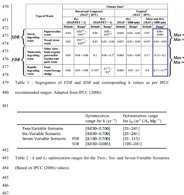
Table 1 - Segregation of FDR and SDR and corresponding k values as per IPCC 99

recommended ranges. Adapted from IPCC (2006). 100

6 of 30

101

These adaptations of the biogas generation modeling process were considered in order to 102

develop a more reliable management tool to predict landfill gas generation. So far, 103

LandGEM has been used at the CESM landfill. 104

By attributing independent values of k and L0 and different fractions between FDR and

105

SDR that best reflected the changing proportions of admitted refuse during the 3 periods

106

mentioned previously, the same first-order model equation used in LandGEM was adapted 107

to generate production curves. Minimization of error between modeled generation and 108

generated gas helped to find the best fitting curve, i.e. the optimized values of k, L0, and

109

fraction of FDR for each period. In an intermediate step, collection data were transformed 110

into generation data by adopting a fixed recovery efficiency rate. 111

The objective is to use the optimized generation curves to predict the optimal moment to 112

shut down the biogas collection system, when the minimum technological threshold (MTT) 113

would be attained. The optimized values of the independent variables were tested against 114

the known history of refuse admittance. In principle, the methodology adopted could be 115

replicated to other landfills, by considering the specific evolution of the FDR fraction in 116

the landfilled waste and the available gas collection database. 117

118

METHODS

119

Landfill gas collection and landfilled mass data

7 of 30

Landfill gas (LFG) collection data were obtained between 1994 and 2013. For this period, 121

yearly compilations were performed using daily biogas collection data. A global relative 122

error of 2.9% was calculated for the flowmeter and chromatograph used to mesure 123

collected CH4 at the CESM landfill (Lagos, 2014). The total landfilled mass was 124

determined on a yearly basis starting in the opening year, in 1968, until its closure, in 2008. 125

The types of refuse admitted were mainly household, commercial, institutional and 126

industrial waste, as well as construction and demolition debris. The latter included inert 127

(non LFG-generating) matter such as, asphalt, concrete and bricks. 128

Transformation from gas collection to generation data

129

Gas collection data were transformed into generation data by setting a recovery efficiency 130

percentage that remained constant throughout the lifetime of the site. The main analysis 131

(presented in detail herein) was performed with an efficiency rate considered as excellent 132

in the literature, i.e. 75% (Spokas et al., 2006; Spokas et al., 2015). Given the proximity of 133

this landfill to housing developments, the presence of an extensive active gas collection 134

system (consisting of over 260 LFG collection wells), and a history of very low measured 135

emissions, high efficiencies can be considered plausible for this specific site (Franzidis et 136

al., 2008; Héroux et al., 2010). According to IPCC (2006), higher than 75% collection 137

efficiencies can only be attributed to properly capped sites with designed and well-138

operated gas recovery systems. In order to evaluate how the year of occurrence of MTT is 139

affected by gas collection efficiency, MTT was obtained for the following recovery 140

efficiency values: 55%, 65%, 75%, 85%, and 95%. 141

8 of 30 Scenarios considered

143

Based on refuse admittance history at CESM – including the ban of landfill organic matter 144

in 2000 – and societal changes triggered by new recycling policies, the lifetime of this site 145

was subdivided into 3 distinct periods: 1968–1989, 1990–1999 and 2000–2008. The 146

extension of period 3 beyond the end of landfilling (2008) is justified by the need to predict 147

methane generation to estimate the year of occurrence of MTT and the onset of aftercare. 148

The beginning of period 3 was easily determined; it coincided with the ban on organic 149

matter (FDR) admittance at CESM, in May 2000. The beginning of period 2 was chosen 150

based on the implementation of recycling programs in the Province of Quebec in the early 151

1990s. Given the fact that it is difficult to identify exactly when recycling programs became 152

effective – therefore affecting the fractions of landfilled FDR and SDR –, the sensitivity of 153

the transition between periods 1 and 2 was tested by setting it 4 years before and 4 years 154

after 1990. This test was performed only for the Seven-Variable Scenario (presented 155

hereafter). 156

Refuse admitted in each of the three periods had particular characteristics that distinguished 157

it. Therefore, the fractions of landfilled FDR and SDR eventually became one of the 158

variables of this parametric study, which was performed based on the following three 159

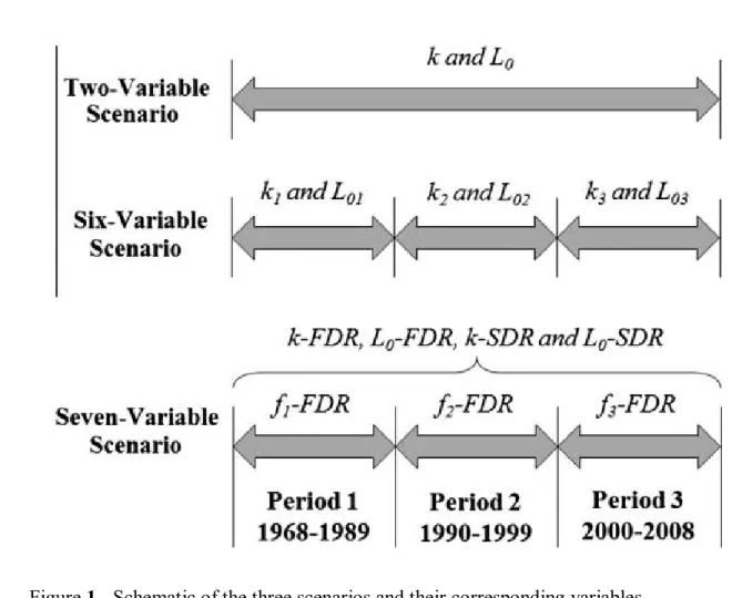
scenarios, illustrated in Figure 1: 1) Two-Variable Scenario, for which one single set of the 160

parameters k and L0 characterized the refuse for the entire lifetime of the site. This scenario

161

corresponds to the current simple phase formulation of LandGEM; 2) Six-Variable 162

Scenario, for which one set of k and L0 values would be selected for the refuse in each of

163

the three key periods; and 3) Seven-Variable Scenario, for which two sets of k and L0 values

164

were adopted: one characterizing FDR and the other SDR. Both sets remained the same 165

9 of 30

throughout the entire study period. However, 3 fractions of FDR in the refuse were adopted, 166

one for each of the 3 key periods. All variables in these 3 scenarios were optimized within 167

predetermined ranges as per IPCC (2006) recommendations. 168

It is obvious that a simple increase in the number of independent variables would lead to 169

an improvement in model fit. But this would be meaningless if the optimization process 170

did not include considerations about what really happened during the history of this 171

landfill, in particular concerning the characteristics of the wastes landfilled. For example, 172

an optimization result indicating that the site saw an increase in FDR over time would not 173

be coherent with the fact that there was a ban in landfilling of organic matter at the 174

beginning of period 3. Such an optimization result would therefore have to be rejected. In 175

short, the 2, 6 or 7 variables in each model are not truly independent as each model must 176

be both internally consistent (i.e. the relative value of each variable must be plausible) and 177

correspond to reality. 178

179

Figure 1 - Schematic of the three scenarios and their corresponding variables. 180

181

Modeling variables and their optimization ranges

182

As shown in Figure 1, variables were labeled in the following manner: 1) k and L0, for the

183

Two-Variable Scenario; 2) k1, k2, k3, L01, L02 and L03, for the Six-Variable Scenario; and 3)

184

L0-FDR, L0-SDR, k-FDR, k-SDR, f1-FDR, f2-FDR and f3-FDR, for the Seven-Variable

10 of 30

Scenario. The subscript n = 1, 2 or 3 denotes the landfilling period to which the variable 186

belongs, while f1, f2 and f3 denote the fractions of FDR in the refuse.

187

The ranges within which k, L0, kn, L0n and fn-FDR could vary during optimization were

188

chosen to allow maximum flexibility while keeping values within IPCC recommended 189

ranges and realistic in relation to the documented landfilling history. Optimization ranges 190

for k and L0 were based on IPCC recommended values for FDR (i.e. food and municipal

191

sludge) and SDR (i.e. cellulose and textiles) (IPCC, 2006). Values for k were taken from 192

the Very Humid Tropical Climate category. This is assumed to be valid, since the CESM 193

landfill is situated in an old quarry, with considerable influx of groundwater (Héroux, 194

2008). L0 values, expressed as DOC, were converted into L0 using equation 1, as follows:

195

𝐿₀ = 𝐹 𝐷𝑂𝐶 𝐷𝑂𝐶_𝑓(16

12) 𝑀𝐶𝐹 (1) 196

where F is the fraction of CH4 in generated landfill gas; DOCf is the fraction of dissimilated

197

organic carbon; 16/12 is the molecular weight ratio of CH4 to C and MCF is the correction 198

factor for aerobic decomposition (IPCC, 2006; Thompson et al., 2009). 199

The value of F was averaged at 0.56 from daily measurements of CH4 and CO2 in the 200

collected landfill gas at CESM between 2001 and 2013. DOCf was set at 0.5 (default value

201

according to IPCC) and MCF at 1.0, as recommended by IPCC (2006) for a site under 202

anaerobic conditions, such as the CESM landfill. Mass units of DOC were then converted 203

to volumetric units using a CH4 volumetric mass of 714 g m-3. While recent work by Wang 204

et al. (2011) shows that DOCf can significantly vary with the nature of waste, the default

11 of 30

IPCC value of 0.5 is considered constant in this study. This fact may be of interest in future 206

studies in order to reduce uncertainties in the transformation of DOC to L0.

207

Table 2 presents k and L0 optimization ranges for the three scenarios. The choice – among

208

IPCC recommendations – of what is considered a very high k value for a North American 209

landfill is partly justified by the high degree of saturation of the refuse. Furthermore, work 210

by De la Cruz and Barlaz (2010) shows that component-specific IPCC-recommended k 211

values for food waste and garden-park waste were underestimated by 200% and 400% 212

respectively. Wang et al. (2013) also concluded that higher values than usually 213

recommended in the literature can be adopted in certain cases. 214

The ranges of values for each of the two categories of waste of the Seven-Variable Scenario 215

(FDR and SDR) were also taken from IPCC (2006). The optimization range of L0

216

corresponds to the minimum and maximum L0 found for the same waste categories

217

considered in FDR and SDR segregation. The maximum and minimum values of k and L0

218

for each category of waste were selected to create a single optimization range. It can be 219

observed that there is some degree of overlapping of FDR and SDR L0 values between 105

220

and 115 m3 _{CH4 Mg}-1_{. In other words, the subdivision into FDR and SDR is not clear-cut.} 221

As mentioned previously, this overlap can be attributed to the generalizations of the trends 222

observed in IPCC-recommended k and L0 values, which are representative of the bulk

223

behaviour of the waste mass and not that of specific components. 224

225

Table 2 - k and L0 optimization ranges for the Two-, Six- and Seven-Variable Scenarios

226

(Based on IPCC (2006) values). 227

12 of 30

228

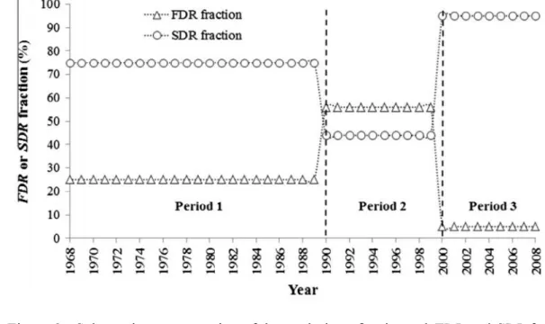
The FDR fractions of the Seven-Variable Scenario were estimated for each of the three 229

periods. For period 2, FDR = 56% and SDR = 44%. These estimates were based on a study 230

that characterized refuse landfilled in 2000, in the Province of Quebec (RECYC-QUÉBEC, 231

2000). For period 3, based on a characterization study performed at the CESM site in 2006 232

(Baillargeon et al., 2006), fractions for FDR and SDR were set at 5% and 95% respectively. 233

Since the contribution of inert matter – such as concrete, asphalt and bricks – in generating 234

LFG is, for all practical purposes, negligible, it was taken out of the mass balance when 235

calculating FDR and SDR fraction estimates. For period 1, no characterization study could 236

be found relating to FDR or SDR fractions. Nonetheless, it was expected that before period 237

2, when recycling had yet to become common practice, a smaller fraction of FDR was 238

landfilled (indeed, greater quantities of paper and cardboard ended up in the landfill). Based 239

on available information, an estimated fraction of 25% was therefore adopted for FDR in 240

period 1. Figure 2 shows the variation of these values throughout the lifespan of the site. 241

Erreur ! Source du renvoi introuvable. presents the optimization ranges for FDR

242

fractions in the Seven-Variable Scenario. The adopted optimization range for the FDR 243

fraction is wide, since it reflects the uncertainty resulting from lack of information for this 244

site, and the estimative nature of characterization studies. Nonetheless, it is worthwhile 245

repeating that the results must be anchored in reality. They must reflect the actual history 246

of landfilling; otherwise, this study would be a mere fitting exercise. 247

13 of 30

Figure 2 - Schematic representation of the evolution of estimated FDR and SDR fractions 249

at CESM from opening (1968) to closure (2008). 250

251

Table 3 - Optimization ranges for FDR fractions in the Seven-Variable Scenario for the 252

three periods considered. 253

254

LandGEM formulation

255

LandGEM is based on the following first-order decomposition rate equation:

256 𝑄𝐶𝐻4𝑛 = ∑ ∑ 𝑘 𝐿0( 𝑀_𝑖 10) 𝑒 −𝑘𝑡𝑖,𝑗 ₍₂₎ 1 𝑗=0.1 𝑛 𝑖=1 257

where QCH4n = annual methane generation in the nth year of the calculation (m3 yr-1); k =

258

methane generation rate (yr-1_{); L}

0 = potential methane generation capacity (m3 Mg-1); Mi =

259

mass of waste accepted in the ith _{year (Mg); tij = age of the j}th _{section of waste mass Mi}

260

accepted in the ith _{year (decimal years); i = 1 year time increment; j = 0.1 year time}

261

increment; and n = number of years in the calculation, i.e. year of calculation – initial year 262

of waste acceptance (USEPA, 2005). 263

For the Six- and Seven-Variable Scenarios, LandGEM calculations were rewritten in an 264

Excel spreadsheet to be able to assign different sets of variables to each of the three periods. 265

Error minimization technique

14 of 30

The sum of squared errors (SSE) between gas collection data and modeled results was 267

minimized by means of the Generalized Reduced Gradient nonlinear method using a 268

commercial spreadsheet. The SSE is described by equation 3, as follows: 269

𝑆𝑆𝐸 = ∑(𝑄𝑚𝑖− 𝑄𝑐𝑖)2 (3) 𝑛

𝑖=1

270

where n = number of yearly values of available collection data; i = year of calculation; Qmi

271

= measured generated methane in the ith _{year (m}3 _yr-1_{); and Qci = generated methane in the} 272

ith _{year calculated by equation 2 (m}3 _yr-1_{) .} 273

The unicity of the optimized results presented herein was evaluated by scanning the model 274

variables within predetermined limits and computing SSE values for each set of selected 275

parameters. This is illustrated in Figure 3, which presents the SSE values for 104 276

combinations of k and L0 values (100×100) of the Two-Variable Scenario, for recovery

277

efficiencies equal to 55%, 75% and 95%. The minimal SSE is found in the region 278

represented by the darkest zone, which was set by an error range within 10% of the SSE. 279

This zone confirms the presence of a single localized minimum. Similar behaviour was 280

obtained for the Six- and Seven-Variable Scenarios. 281

282

Figure 3 – Model-predicted errors for the Two-Variable Scenario as function of recovery 283

efficiency. 284

15 of 30

RESULTS AND DISCUSSIONS

286

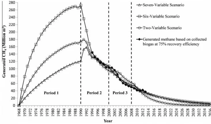
Figure 4 shows CH4 generation obtained by the reformulated LandGEM equation, for the 287

three scenarios considered. The curve with solid points represents data collected from 1994 288

to 2013 that were transformed into generation values by considering 75% recovery 289

efficiency. The lowest SSE value was obtained for the Six-Variable Scenario. Accordingly, 290

the best fit with generation data (based on actual collection) was obtained for this scenario. 291

It was followed by the Seven-Variable and Two-Variable Scenarios with respective SSE 292

values 2.6 and 6.3 times higher. 293

294

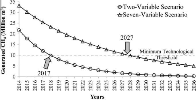
Scenarios were analyzed in terms of their ability to predict when the MTT would be 295

attained. In the case of the CESM landfill facility, MTT is approximately 10 Mm3 _yr-1_. 296

Below this value, LFG collection would no longer be sustainable with the present gas 297

collection system. 298

299

Figure 4 - Modeled CH4 generation for the Two-, Six- and Seven-Variable Scenarios as 300

optimized after SSE minimization relative to measured CH4 generation. 301

302

Two-Variable Scenario

303

This scenario considers a single type of refuse admitted throughout the landfill’s operating

304

life. According to this scenario, the MTT would be reached in 2017. Based on latest 305

available data (2012 and 2013), CH4 generation seems to be underestimated. 306

16 of 30

Values of k and L0 optimized by SSE minimization were 0.197 yr-1 and 127 m3 CH4 Mg-1 307

respectively. The relatively high k and low L0 would indicate a refuse with a high

308

proportion of FDR, which is not necessarily the case for the refuse landfilled at the CESM 309

site. This is an indication that this model does not coincide with actual landfill history and 310

therefore needs refining. 311

Six-Variable Scenario

312

This scenario also considers a single type of refuse but landfilling was subdivided into the 313

three periods indicated in Erreur ! Source du renvoi introuvable.; each with its own

314

independently optimized values of k and L0. Since the optimization ranges for k and L0

315

were the same for all three periods, these variables were free to increase or decrease from 316

one period to the next. 317

Optimized values for k1, k2, k3, L01, L02 andL03 were 0.282 yr-1, 0.081 yr-1, 0.030 yr-1, 194

318

m3 _CH

4 Mg-1, 241 m3 CH4 Mg-1 and 21 m3 CH4 Mg-1 respectively. The decrease in 319

optimized k values – and increase in L0 values – between periods 1 and 2 implies that the

320

fraction of FDR within the waste would also have decreased. Yet this is not corroborated 321

by historical data. Indeed, recycling programs deployed in the early 1990s led to an 322

important decrease in landfilling of paper and cardboard (SDR fraction), which caused an 323

increase in the fraction of FDR in subsequent years (Figure 2). 324

Values of optimized L0 decreased between periods 2 and 3, implying that the fraction of

325

SDR would also have decreased. Again, this trend is not backed up by the CESM landfilling

326

history. In 2000, CESM forbade admission of FDR, such as household waste, hence 327

increasing SDR fractions. These mismatches between optimization of the variables and 328

17 of 30

known refuse admittance history suggest that the Six-Variable Scenario could not be 329

retained, despite the fact that the lowest SSE value was obtained with it. Furthermore, 330

before 1992 the modeled curve seems to greatly overestimate CH4 generation in 331

comparison with the other two scenarios with a ~ 100 Mm3 _{difference at generation peak} 332

in 1990. Such an additional volume of landfill gas seems unlikely given the environmental 333

nuisances that would have resulted for workers and the surrounding population; a nuisance 334

that was never observed. Accordingly, the Six-Variable Scenario was deemed 335

inappropriate to explain the behaviour of LFG generation for this site. According to the 336

Six-Variable Scenario, the MTT would be reached in 2028. 337

Seven-Variable Scenario

338

This scenario considers two types of refuse and their fractions that vary along the three 339

periods indicated in Erreur ! Source du renvoi introuvable.. Since the optimization

340

ranges for the FDR fractions shown in Erreur ! Source du renvoi introuvable. are

341

different but overlap between periods 1 and 2, optimized fn-FDR could increase or decrease

342

along these periods. The optimization ranges for the FDR were different and decreased 343

from period 2 to period 3. Accordingly, optimized fn-FDR was expected to decrease from

344

period 2 to period 3. 345

Optimized values for k-FDR, k-SDR, L0-FDR, L0-SDR were, 0.363 yr-1, 0.085 yr-1, 115 m3

346

CH4 Mg-1, 105 m3 CH4 Mg-1, respectively. Moreover, the optimized values for f1-FDR, f2

-347

FDR and f3-FDR were 11%, 70% and 5%, respectively. Contrary to the Six-Variable

348

Scenario, there is no mismatch between optimized FDR and SDR fractions and the history 349

of refuse admittance. The value of optimized k-SDR is nearly four times lower than that of 350

18 of 30

k-FDR and the value of optimized L0-SDR is moderately higher than that of L0-FDR.

351

According to the Seven-Variable Scenario, the MTT would be reached by 2027. 352

353

The Seven-Variable Scenario allows for consideration of changes in landfilling trends, as 354

reflected in variations of FDR and SDR fractions. This is a clear added-value to the simple 355

phase Two-Variable Scenario. In addition, contrary to the Six-Variable Scenario, the 356

optimized variables of the Seven-Variable Scenario better reflect the landfilling history. 357

For these reasons, the year 2027 – when the Seven-Variable Scenario is expected to reach 358

the MTT – is a more reliable prediction for gas collection shutdown. Figure 5 shows MTT 359

for the Two- and Seven-Variable Scenarios. 360

361

Figure 5 – Minimun Technological Threshold for the Two- and the Seven-Variable 362

Scenarios. 363

364

Effect of the variation of landfill gas recovery efficiency

365

The results presented above were obtained by adopting 75% recovery efficiency 366

throughout the lifetime of the CESM landfill. The effect of recovery efficiency on the MTT 367

year of occurrence and on the SSE for the three scenarios was tested by varying it from 368

55% to 95% in increments of 10 percentage points. At each increment, a new optimization 369

was performed for each scenario. The results obtained are presented in Figure 6, which 370

shows that when the recovery efficiency is increased from 75% to 95%, the MTT occurs 371

19 of 30

1, 3 and 2 years earlier, for the Two-, Six- and Seven-Variable Scenarios, respectively. For 372

all practical purposes, these differences can be considered relatively small. The results of 373

Figure 6 also show that, regardless of the value of the recovery efficiency, the Six-Variable 374

Scenario consistently had the lowest SSE. The decrease in SSE becomes smaller as 375

recovery efficiency increases and seems to level off when the recovery efficiency reaches 376

75%. 377

Although not apparent in the results presented in Figure 6, our analyses show that for all 378

tested efficiencies, the Seven-Variable Scenario seemed to better reflect the landfilling 379

history at the Montreal-CESM landfill, while the Six-Variable Scenario presented the same 380

discrepancy between optimized values and landfilling history, as previously mentioned. 381

High LFG recovery efficiencies are expected in this landfill due to the more than 250 382

biogas collection wells installed. Numerous surface and lateral migration surveys have 383

shown that surface fluxes have been very low. It is up to the operator to consider the 384

efficiency level he/she feels comfortable with when estimating the year of occurrence of 385

MTT for this particular site. 386

387

Figure 6 – MTT year of occurrence (a) and SSE (b) as a function of recovery efficiency. 388

389

Effect of start of transition year between periods 1 and 2

20 of 30

The sensitivity of the choice made for the transition year between periods 1 and 2 – when 391

recycling programs became effective, therefore affecting landfilled FDR and SDR fractions 392

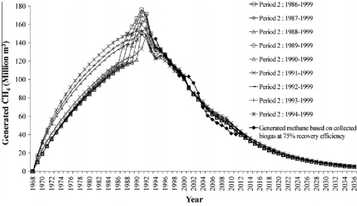
– was assessed for the Seven-Variable Scenario and for 95% recovery efficiency. Figure 7 393

shows the effect of moving the end-of-period four years back or forward, relative to 1990. 394

As the limit year was moved from 1986 to 1994, there was a minimal effect on modeled 395

generation values after the generation peak. 396

397

Figure 7 - Effect of the variation of the limit year between periods 1 and 2 on the 398

modeling of CH4 generation for the Seven-Variable Scenario. 399

400

FURTHER DISCUSSIONS AND LIMITATIONS

401

The method proposed in this study accounts for the variation in the nature of admitted 402

refuse at landfill sites, which is a consequence of changes in the environmental 403

consciousness of societies – in turn reflected in stricter regulations – and the economics of 404

waste management. Consideration of how these socio-economic changes affect landfill gas 405

generation is crucial when it comes to making decisions about the fate of systems put in 406

place to reduce the environmental impact of landfills and increase their economic viability. 407

Errors associated with measurements of various gas concentrations at the CESM landfill 408

can be considered minor, due, in part, to continuous gas quality monitoring and the quality 409

control assured by the well-equipped laboratory on site. However, high operational 410

variances may have caused the bumps in the generation curve observable in the years 2000 411

21 of 30

and 2012 (Figure 4). These variances can be attributed to a myriad of causes, including: re-412

excavation and re-landfilling of waste, temporary difficulties with the gas or leachate 413

collection systems (such as defective wells), localized settlements, localized elevated 414

temperatures, etc. Consideration of variable recovery efficiency could account, at least in 415

part, for the operational variances; hence the interest in considering it in further works. As 416

shown in this study, these limitations did not seem to influence the fact that the Seven-417

Variable Scenario was found to be the most appropriate scenario to estimate shutdown 418

time, despite the fact that its minimization error was not the lowest. 419

420

ACKNOWLEDGEMENTS

421

This study received financial support from the Université de Sherbrooke’s Center of 422

Excellence GREEN-TPV, and the Natural Science and Engineering Research Council of 423

Canada (NSERC), under Discovery Grants RGPIN-170226-2013 and

424 RGPIN-402368-2011. 425 426

REFERENCES

Baillargeon, A., Bisson, M., Blouin, V., Mercure, A., Séguin, M., Guimond, J.Y., 2006. 428

Characterization study of the wastes landfilled at CESM (in French: Étude de 429

caractérisation des chargements entrant au CESM). City of Montreal (Ville de Montreal), 430

Montreal, QC, p. 21. 431

22 of 30

De la Cruz, F.B., Barlaz, M.A., 2010. Estimation of waste component-specific landfill 432

decay rates using laboratory-scale decomposition data. Environ. Sci. Technol. 44, 433

4722−4728. 434

Franzidis, J.P., Héroux, M., Nastev, M., Guy, C., 2008. Lateral Migration and Offsite 435

Surface Emission of Landfill Gas at City of Montreal Landfill Site. Waste Management & 436

Research 26, 121-131. 437

Héroux, M., 2008. Développement d'outils de gestion des biogaz produits par les lieux 438

d'enfouissement sanitaire (in French. Translation of title: Development of Landfill Biogas 439

Management Tools), Génie minéral. École Polytechnique de Montréal, Montreal, Quebec, 440

p. 281. 441

Héroux, M., Guy, C., Millette, D., 2010. A Statistical Model for Landfill Surface 442

Emissions. Journal of Air & Waste Management Association 60, 219-228. 443

IPCC, 2006. Guidelines for National Greenhouse Gas Inventories, in: Eggleston, S., 444

Buendia, L., Miwa, K., Ngara, T., Tanabe, K. (Eds.), Hayama, Japan. 445

Lagos, D.A., 2014. Optimisation du modèle de génération de méthane du lieu 446

d’enfouissement du complexe environnemental de Saint-Michel, CUFE. Université de 447

Sherbrooke, Sherbrooke, p. 80. 448

RECYC-QUÉBEC, 2000. Bilan 2000 de la gestion des matières résiduelles au Québec, p. 449

30. 450

Spokas, K., Bogner, J., Chanton, J.P., Morcet, M., Aran, C., Graff, C., Golvan, Y.M.-L., 451

Hebe, I., 2006. Methane mass balance at three landfill sites: What is the efficiency of 452

capture by gas collection systems? Waste Management 26, 516-525. 453

23 of 30

Spokas, K., Bogner, J., Corcoran, M., Walker, S., 2015. From California dreaming to 454

California data: Challenging historic models for landfi ll CH4 emissions. Elementa: Science 455

of the Anthropocene 3, 16. 456

Thompson, S., Sawyer, J., Bonam, R., Valdivia, J.E., 2009. Building a better methane 457

generation model: Validating models with methane recovery rates from 35 Canadian 458

landfills. Waste Management 29, 2085-2091. 459

USEPA, 2005. Landfill Gas Emissions Model (LandGEM) Version 3.02 User’s Guide. 460

United States Environmental Protection Agency, Washington, D.C., p. 56. 461

Wang, X., Nagpure, A.S., DeCarolis, J.F., Barlaz, M.A., 2013. Using Observed Data to 462

Improve Estimated Methane Collection from Select U.S. Landfills. Environmental Science 463

and Technology 47, 3251-3257. 464

Wang, X., Padgett, J.M., De la Cruz, F.B., Barlaz, M.A., 2011. Wood Biodegradation in 465

Laboratory-Scale Landfills. Environ. Sci. Technol. 45, 6864-6871. 466

467 468

24 of 30 List of Tables 469 470 471 472 473 474 475 476 477 478

Table 1 - Segregation of FDR and SDR and corresponding k values as per IPCC 479

recommended ranges. Adapted from IPCC (2006). 480

481

482

Table 2 - k and L0 optimization ranges for the Two-, Six- and Seven-Variable Scenarios

483

(Based on IPCC (2006) values). 484

485 486 487

25 of 30

488

Table 3 - Optimization ranges for FDR fractions in the Seven-Variable Scenario for the 489

three periods considered. 490

491 492 493 494

26 of 30 List of Figures

495 496

497

Figure 1 - Schematic of the three scenarios and their corresponding variables.

498 499

27 of 30

500

Figure 2 - Schematic representation of the evolution of estimated FDR and SDR fractions

501

at CESM from opening (1968) to closure (2008). 502

503

504

Figure 3 – Model-predicted errors for the Two-Variable Scenario as function of recovery 505

efficiency. 506

28 of 30

507

Figure 4 - Modeled CH4 generation for the Two-, Six- and Seven-Variable Scenarios as 508

optimized after SSE minimization relative to measured CH4 generation. 509

510 511 512

29 of 30

513

Figure 5 – Minimun Technological Threshold for the Two- and the Seven-Variable 514

Scenarios. 515

516

Figure 6 – MTT year of occurrence (a) and SSE (b) as a function of recovery efficiency.

30 of 30

518

Figure 7 - Effect of the variation of the limit year between periods 1 and 2 on the

519

modeling of CH4 generation for the Seven-Variable Scenario. 520