To cite this document:
Escrig, Benoît Estimation of Collision Multiplicities in IEEE 802.11-based WLANs.
(2012) In: The 11th International Conference on Networks (ICN), 2012, 29 Feb - 5
Mar 2012, Reunion Island, France.
O
pen
A
rchive
T
oulouse
A
rchive
O
uverte (
OATAO
)
OATAO is an open access repository that collects the work of Toulouse researchers and
makes it freely available over the web where possible.
This is an author-deposited version published in:
http://oatao.univ-toulouse.fr/
Eprints ID: 5901
Official URL:
http://www.thinkmind.org/index.php?view=article&articleid=icn_2012_9_10_10081
Any correspondence concerning this service should be sent to the repository
administrator:
[email protected]
Estimation of Collision Multiplicities in
IEEE 802.11-based WLANs
Benoˆıt Escrig
IRIT Laboratory
Universit´e de Toulouse
Toulouse, France
E-mail: [email protected]
Abstract—Estimating the collision multiplicity (CM), i.e. the number of users involved in a collision, is a key task in multi-packet reception (MPR) approaches and in collision resolution (CR) techniques. A new technique is proposed for IEEE 802.11 networks. The technique is based on recent advances in random matrix theory and rely on eigenvalue statistics. Provided that the eigenvalues of the covariance matrix of the observations are above a given threshold, signal eigenvalues can be separated from noise eigenvalues since their respective probability density functions are converging toward two different laws: a Gaussian law for the signal eigenvalues and a Tracy-Widom law for the noise eigen-values. The proposed technique outperforms current estimation techniques in terms of underestimation rate. Moreover, this paper reveals that, contrary to what is generally assumed in current MPR techniques, a single observation of the colliding signals is far from being sufficient to perform a reliable CM estimation.
Index Terms—multi-packet reception; collision multiplicity; model order selection; IEEE 802.11-based networks
I. INTRODUCTION
The throughput of IEEE 802.11-based networks highly depends on the number of collisions. When the number of col-lisions increases, the throughput is degraded. Recent advances in multi-user detection (MUD) now allow the processing of collision signals, so data packets from collided user terminals can be successfully decoded at the access point even when a collision occurs. One [1], [2] or several [3], [4] transmissions from the colliding users are needed in order to achieve the decoding of the packets. The first step that is performed by these multi-packet reception (MPR) techniques consists of estimating the number of users involved in the collision: the collision multiplicity (CM). The estimation process im-plements a well-established Model Order Selection Technique (MOST) [5]. First, an eigenvalue decomposition is performed on the sample covariance matrix (SCM) of the observations (”snapshots”). Then, the well-known information criterion MDL (Minimum Description Length) is applied in order to perform the CM estimation. In the context of wireless local areas networks (WLANs), current CM estimation techniques (CMETs) are based on the following two assumptions: (i) the signal samples are uniformly distributed, i.e., signal samples are either PSK or QAM modulation symbols, and (ii) the num-ber of snapshots is not much greater that the CM [1], [2], [6]. These two assumptions are rather questionable when applied to IEEE 802.11-based networks. First, the IEEE 802.11 standard
relies on orthogonal frequency division multiplex (ODFM) transmissions so signal samples are not uniformly distributed but rather distributed according to a Gaussian law. Second, the assumption of a low number of observations (compared to the CM value) contradicts typical assumptions in MOSTs [7], [8]. In this paper, we propose a new CMET, denoted as TWIT (Tracy-Widom Inference Test). Simulation results show that the TWIT outperforms the classical MDL in the context of IEEE 802.11-based WLANs. Moreover, we show that the number of observations that are needed to perform the CM estimation is far much grater than the one that is used in CMETs.
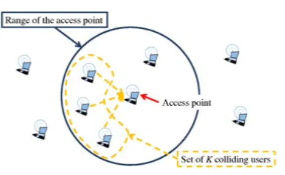
Fig. 1. Collision Scenario with K = 3 colliding users.
The rest of the paper is organized as follows. The sys-tem model is introduced in Section II and some results on eigenvalue statistics are stated in Section III. The CMETs are described in Section IV. Simulation results are presented in Section V and a conclusion is drawn in the last section.
II. SYSTEMMODEL
In the proposed scenario, K users are simultaneously trans-mitting OFDM frames toward an AP. Each OFDM frame contains m symbols. The OFDM signal samples are Gaussian distributed and have a white power spectral density. For sake
of simplicity, the AP and the user terminals are assumed to be equipped with a single antenna. The AP can trigger retrans-missions from the colliding users by transmitting a feedback frame. The signaling frame serves also as a synchronization flag for user transmissions. When T snapshots are available at the AP, the T × 1 observation vector yi is written as
yi= Hsi+ wi, i = 0, 1, . . . , m
where m denotes the number of samples per snapshot, si∼ CNK(0, Rs) are K × 1 complex Gaussian
vec-tors of OFDM samples with covariance matrix Rs and
wi∼ CNT(0, Σ) are T × 1 complex Gaussian noise vectors
with noise covariance matrix Σ. In the white noise case, the covariance Σ is σ2IT where IT is the T × T identity matrix.
The channel matrix H is a T × K matrix with circularly symmetric Gaussian elements with power unity (Rayleigh fading). A block-fading wireless channel is considered here so the coefficients in H have constant values during an OFDM block of m samples, and then change randomly from one block to another. So the channel matrix H is considered as an unknown non-random matrix. When the noise covariance matrix Σ is known a priori and is nonsingular, the snapshots yi can be ”whitened” by the following transformation
y†i = Σ−1/2yi
where Σ−1/2is the Hermitian nonnegative definite square root of Σ. This transformation simply reduces to a normalization step in the case of a white Gaussian noise.
The signal and noise vectors being independent, the covari-ance matrix R of the snapshots yi is given by
R = HRsH∗+ Σ
with ∗ denoting the complex conjugate. We assume that the matrix H is full rank and that the signal covariance matrix Rs
is nonsingular. Hence the rank of HRsH∗ is min(K, T ), i.e.,
HRsH∗has exactly T non-zero eigenvalues when T ≤ K and
K non-zero eigenvalues when T > K. When the whitening transformation is applied, the covariance matrix R† of the whitened snapshots is defined as
R† = Σ−1/2RΣ−1/2= Σ−1/2HRsH∗Σ−1/2+ IT
Let λ1≥ λ2≥ ... ≥ λT denote the population eigenvalues of
R†. We have that
λi> 1 for 1 ≤ i ≤ min(K, T ) (1)
λi= 1 for min(K, T ) < i ≤ T (2)
When R and Σ are known, and when the rank of Σ−1/2HRsH∗ is K, the CM estimation can be easily
per-formed from the multiplicity of the λi equalling one. When
R and Σ are unknown and have to be estimated, another approach must be used. We define the sample covariance matrix (SCM) of the snapshots yi, denoted bR, by
b R = 1 m m X i=1 yiy∗i
and the SCM bΣ of the noise by
b Σ = 1 N N X j=1 wjwj∗
where the wj, 1 ≤ j ≤ N are independent noise-only samples.
We assume that the noise variance σ2 can be estimated by
different other means at the AP when σ2is the only parameter that is needed. Empty time slots can provide the N samples that are needed to compute the SCM bΣ. When the yi are
constituted of simultaneous transmissions from K users, we aim at estimating K based on the eigenvalues of bR†
b
R†= bΣ−1/2R bbΣ−1/2
Let ˆλ1≥ ˆλ2≥ ... ≥ ˆλT denote the sample eigenvalues of bR†.
III. SOMERESULTS ONEIGENVALUESTATISTICS Eigenvalue-based MOSTs rely on hypothesis tests on eigen-values or on the computation of information criteria. In this paper, we concentrate on the population eigenvalues of bR†. According to (1) and (2), signal eigenvalues (ˆλi > 1) and
noise eigenvalues (ˆλi= 1) could be separated by counting the
number of eigenvalues strictly above one. Recent advances in RMT have shown that it exists a threshold below, which it is not possible to separate signal eigenvalues from noise eigenvalues. More precisely, this threshold being strictly higher than one, each signal eigenvalue between the threshold and one will be considered as being a noise eigenvalue, thus misleading typical eigenvalue-based MOSTs. Moreover, increasing the number of observations will exacerbate the phenomenon since the threshold increases with the number of observations. In this section, we present several properties on the eigenvalues and characterize the threshold issue.
Property 3.1: Let X be a T × m matrix constituted of m samples. The samples are drawn from a T -dimensional complex Gaussian law CNT(0, Σ). Let A = XXH. Let
CWT(m, Σ) denote the T -variate complex Wishart law with
m degrees of freedom. From [9], we have that A ∼ CWT(m, Σ)
Property 3.2: Let A ∼ CWT(m, Σ) be independent of
B ∼ CWT(N, Σ) where m, N > T . In the case of a double
Wishart setting, we search for the eigenvalues θ that satisfy
Av = θ(A + B)v (3)
where v denotes the eigenvector corresponding to the eigen-value θ. Let λ[(A+B)
−1A]
1 be the largest eigenvalue satisfying
(3). When m, N → ∞ as T → ∞ with m, N > T , we have that
P[W (λ
[(A+B)−1A]
1 ) − µ(T, N, m)
σ(T, N, m) ≤ x] → T WC(x) where T WC(x) is the Tracy-Widom distribution function for complex data and W (θ) denotes the logit transformation of θ,
i.e., W (θ) = log[θ/(1 − θ)] and β = min(N, T ) γ = m − T δ = |N − T | µ(T, N, m) = (uβ τβ +uβ−1 τβ−1 )(1 τβ + 1 τβ−1 )−1 σ(T, N, m) = 2(1 τβ + 1 τβ−1 )−1 sin2(γβ/2) = (β + 1/2) × (2β + γ + δ + 1)−1 sin2(φβ/2) = (β + δ + 1/2) × (2β + γ + δ + 1)−1 τβ3 = 16(2β + γ + δ + 1)−2 × sin−2(φβ+ γβ) × sin−1(φβ) sin−1(γβ) uβ = 2 log[tan( φβ+ γβ 2 )]
Property 3.2 has been proved for Σ = IT but the property can
be applied to any Σ since the covariance matrix has no effect on the distribution of the eigenvalues [10].
Rewriting (3) for θ = λ[(A+B)
−1A] 1 , we have that AB−1v = λ [(A+B)−1A] 1 1 − λ[(A+B)1 −1A] v
Property 3.3: Let A ∼ CWT(m, Σ) be independent of
B ∼ CWT(N, Σ) where m > T . The largest eigenvalue of
AB−1, denoted λ(AB −1) 1 , satisfies P{log[λ (AB−1) 1 ] − µ(T, N, m) σ(T, N, m) ≤ x} → T WC(x) when m, N → ∞ as T → ∞. A. Signal-free Case
In the signal-free case, no user is transmitting, so K = 0. As a consequence, R = Σ, R† = IT, and all the population
eigenvalues λi are equal to 1. Moreover, when the number
of observations T is fixed and when m, N → ∞, the sample eigenvalues ˆλi are symmetrically centered around the
population eigenvalues λi for i = 1, . . . , T . In the T, m → ∞
asymptotic regime, the spreading of the sample eigenvalues can be characterized by the empirical distribution function (edf) [9], [11]–[13].
Property 3.4: In the signal-free case, when all the popula-tion eigenvalues λi are equal to 1, when T, m → ∞ such that
T /m → c ∈ (0, ∞), the limiting edf of the sample eigenvalues ˆ λi is given by 1/T #{ˆλi: ˆλi≤ x} → H(x) where dH(x) = max (0, (1 − 1 c))δ(x) + 1 2πxc p (b − x)(x − a)1a,b(x)dx
with a = (1 −√c)2, b = (1 +√c)2, and 1a,b(x) = 1 when
a ≤ x ≤ b.
The probability density function (pdf) dH(x) is the Mar˘ cenko-Pastur density. From this property, a first characterization of the ˆλ1 distribution can be inferred [9], [14].
Property 3.5: In the signal-free case, the whitened snap-shots y†i are NT(0, IT) and the largest eigenvalue ˆλ1 of the
SCM bR† is Tracy-Widom distributed. When T, m → ∞ such that T /m → c ∈ (0, ∞), P[mˆλ1− µT ,m σT ,m ≤ x] → T WC(x) where µT ,m = ( √ T +√m)2 σT ,m = ( √ T +√m)(√1 T + 1 √ m) 1/3
When the snapshots yi† are NT(0, σ2IT), the convergence
limit of mˆλ1 is σ2(
√
T + √m)2. This corresponds to the
non-normalized case. Note that the convergence rate to the T WC(x) distribution function is O(T−1/3). When the pa-rameters m and T are not so large, which is practically the case when we want to reduce the number of observations, the convergence rate to the Tracy-Widom distribution is rather O(T−2/3) provided that the mean and standard deviation have
been modified appropriately [9], [10].
From Property 3.2, we have that N bΣ ∼ CWT(N, Σ) and
m bR ∼ CWT(m, R). We search for the largest eigenvalue ˆλ1
that satisfies b Rv = ˆλ1Σvb or, equivalently (m bR)v = m N ˆ λ1(N bΣ)v
So, using Property 3.3, we have that P{log(
m
Nλˆ1) − µ(T, m, N )
σ(T, m, N ) ≤ x} → T WC(x) B. Signal Bearing Case
When there are K signals and when T → ∞, the limiting edf of bR† still converges to a Mar˘cenko-Pastur distribution. Moreover, the ith largest eigenvalue ˆλ
i converges to a limit
different from that in the signal-free case if and only if the signal eigenvalue is above a certain threshold [12].
Property 3.6: In the signal bearing case, when T → ∞, ˆ λi= ( λi(1 + λc i−1) if λi > (1 + √ c) (1 +√c)2 if λi ≤ (1 + √ c)
When K T , the signal eigenvalues strictly below the threshold (1+√c) exhibit, on rescaling, fluctuations described by the Tracy-Widom distributions, i.e., the signal eigenvalues are closely approximated by the distributions obtained for the signal-free case (K = 0). For signal eigenvalues above the
threshold [11], the fluctuations about the asymptotic limit are Gaussian distributed P[ ˆ λi− µi σi ≤ x] → G(x) where µi = λi(1 + c λi− 1 ) σi = λi √ T r 1 − c (λi− 1)2 and G(x) = Z x −∞ 1 √ 2πexp (− y2 2 )dy
In the T, m → ∞ asymptotic regime with T /m → c ∈ (0, ∞), if signal eigenvalues are below the threshold, then reliable sample-eigenvalue-based detection is not possible. Note that adding more observations does not solve the problem since the threshold is increasing with T . Inversely, when signal eigenvalues are above the threshold, then reliable detection is possible. Note that these properties hold for large T and relatively large m. For lower T and m, the eigenvalues are more fluctuating, so the CM estimation is less reliable.
IV. COLLISIONMULTIPLICITYESTIMATIONTECHNIQUES We assume that the AP has collected T snapshots. First, the SCM of the whitened snapshots is computed. Then, the eigenvalue decomposition of the SCM is performed and the eigenvalues are sorted. The eigenvalues are processed with two CMETs: the first one is based on eigenvalue statistics and the second one relies on information criteria.
A. CMET based on eigenvalue statistics
The proposed algorithm relies on the eigenvalue statistics that have been stated in the previous section. Basically the estimate ˆKTWIT is initialized to zero and incremented by one
for each iteration as long as the eigenvalue ˆλKˆTWIT+1 is not
considered as being an eigenvalue of the noise subspace, i.e., as being Tracy-Widom distributed. The TWIT algorithm is detailed in Algorithm 1. The mean µ(x, y, z) and the standard Algorithm 1 TWIT algorithm
Compute bR†
Compute and sort the eigenvalues ˆλi, i = 1, . . . , T of bR†
ˆ
KTWIT← 0 and T est ← F alse
while T est = F alse and ˆKTWIT< T do
µ ← µ(T − ˆKTWIT, m, N )
σ ← σ(T − ˆKTWIT, m, N )
T est ← {σ−1[log(mˆλ ˆ
KTWIT+1/N ) − µ] < τα}
if T est = F alse then ˆ KTWIT← ˆKTWIT+ 1 else break end if end while
deviation σ(x, y, z) in the algorithm are defined in Property 3.2. Similar expressions can be found for the case of real-valued data. The threshold τα is defined as T WC−1(1 − α)
where α is some significance level. Note that this criterion has been originally designed for arbitrary (or colored) noise [13]. That is the reason why the algorithm uses the eigenvalues of bR†.
B. CMET based on information criteria
Information criteria, such as the MDL or the Aka¨ıke’s information criterion (AIC), have been originally designed in order to avoid subjective threshold settings in MOSTs [7]. The MDL has been widely used over the past two decades and is still used in current CMETs. We shall not refer to the AIC hereafter since the criterion has been proven to be inconsistent in the m → ∞ sense [7]. The MDL criterion is defined as
ˆ KMDL= argmin k=1,...,T {MDL(k)} where MDL(k) = −m(T − k) log[g(k) a(k)] + 1 2k(2T − k) log(m) where g(k) = T Y i=k+1 ˆ λ 1 T −k i a(k) = 1 T − k T X i=k+1 ˆ λi
where the ˆλi denote the eigenvalues of bR† with 1 ≤ i ≤ T .
This estimator is consistent in the m → ∞ sense. One of the reason why the MDL criterion has been widely used over the past two decades comes from its robustness to model mismatch, in particular when the underlying assumptions of snapshots and noise Gaussianity can be relaxed [15]–[17].
V. SIMULATIONRESULTS
CMETs are compared in the context of Rayleigh fading channels. User stations are transmitting OFDM signals that are built according to the IEEE 802.11 standard [18]. The signals are composed of 1024 sub-carriers (Nsub = 1024) and use
BPSK modulation, the guard interval is 1/4 of the total symbol period (GI = 1/4). There are 48 OFDM symbols per OFDM block (NOFDM = 48), so the total number of samples per
snapshot is m = 61440. For sake of simplicity, we have chosen the same number for N , i.e., N = 61440. The performance of CMETs have been evaluated over 10000 Monte Carlo trials.
Figures 2 and 3 show the simulations results for two CMETs: the MDL criterion and the TWIT. The results have been obtained for a fixed number of signals K = 4, a variable number of snapshots 4 ≤ T ≤ 32, and two typical values of the signal to noise ratio SN R: a low value (10 dB) and a high value (30 dB). The significance level α for the TWIT is set to 0.01 [13]. The first figure shows the estimated values of K. The second figure shows the underestimation rate, i.e.,
P[ ˆK < K]. The TWIT outperforms the MDL criterion since it provides similar results with less observations, and so for any value of SN R. Another important result is that T should be significantly larger than K in order to achieve relevant performance levels, i.e. underestimation rate much lower than 10 %.
Fig. 2. Estimates of K = 4 for a variable number of snapshots T , 4 ≤ T ≤ 32.
Fig. 3. Underestimation rate for K = 4 and a variable number of snapshots T , 4 ≤ T ≤ 32.
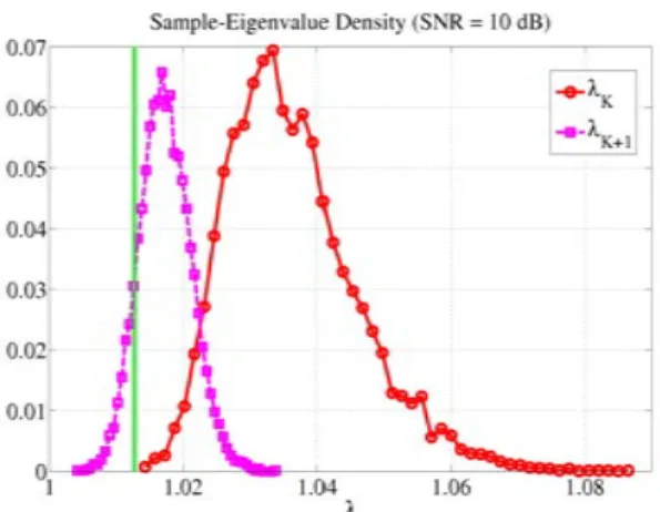
Figures 4 to 6 show the pdfs of the eigenvalues ˆλK and
ˆ
λK+1 for K = 4. These statistics have been obtained with
10000 draws. The pdf of ˆλK represents the pdf of the lowest
”signal” eigenvalue whereas the pdf of ˆλK+1 represents the
pdf of the largest ”noise” eigenvalue.
Figures 4 and 5 show the eigenvalue statistics for T = 10 and two values of the signal to noise ratio, 10 and 20 dB. On these two figures, the lowest signal eigenvalue is always higher than the detectability threshold so all the signal eigenvalues are detectable. However, the pdfs of the signal and the noise eigenvalues are overlapping for SN R = 10 dB. That explains the degradation on the underestimation rate on Fig. 3.
Figures 4 and 6 show the eigenvalue statistics for SN R = 10 dB and two values for T : 10 and 30. The spreading of the pdfs depends on T . The higher is T , the shaper are the density curves. Here again, the performance of the CMET is improving when the number of observations is increasing.
Fig. 4. Estimated probability density functions of the eigenvalues ˆλK and ˆ
λK+1for K = 4, T = 10 and SN R = 10 dB, given that ˆλK∼ bG(λ) and ˆ
λK+1∼ dT W (λ). The vertical line depicts the position of the detectability threshold 1 +√c.
Fig. 5. Estimated probability density functions of the eigenvalues ˆλK and ˆ
λK+1for K = 4, T = 10 and SN R = 20 dB, given that ˆλK∼ bG(λ) and ˆ
λK+1∼ dT W (λ). The vertical line depicts the position of the detectability threshold 1 +√c.
A. Discussion
The simulation results suggest that the CMETs perform well when the number of snapshots is much larger than the number of signals. However, in many current CMETs, the number of snapshots is set to a value close to K. In [3], [4], T is set to a value not greater than K + 1 or K + 2. More surprisingly, in [1], [2], a single transmission of the colliding users is required to proceed to the user separation, using the blind separation technique in [6]. Note that, in [6], the number of sources (users) is assumed to be known or to have been estimated using information criteria such as the MDL criterion. The simulation results presented in this paper are in stark contrast with the settings that are used in these papers. Note also that typical MOSTs rely on similar settings, i.e., T K (see [12] and the reference therein).
Fig. 6. Estimated probability density functions of the eigenvalues ˆλK and ˆ
λK+1for K = 4, T = 30 and SN R = 10 dB, given that ˆλK∼ bG(λ) and ˆ
λK+1∼ dT W (λ). The vertical line depicts the position of the detectability threshold 1 +√c.
VI. CONCLUSION
In this paper, a new CMET, denoted TWIT, has been proposed. The method is based on eigenvalue statistics. Eigen-values are tested in descending order, from the largest to the lowest. The first eigenvalue ˆλq that is considered as
being Tracy-Widom distributed allows the CM estimation by ˆK = q − 1. This CMET has been shown to outperform the typical MDL criterion. Moreover, simulation results have shown that a large number of snapshots T is needed in order to allow a good estimation of K in terms of underestimation rates. Furthermore, the number of snapshots must be signifi-cantly higher than the number of colliding users K (T K). These settings are similar to the settings that are used in MOSTs for signal array processing.
The impact of these results is twofold. First, some CR techniques such as the network-assisted diversity multiple ac-cess (NDMA) [3], [4] cannot be implemented in IEEE 802.11 networks notably because these CR techniques are based on the assumption that T can be made as small as K + 1 or K + 2. Second, some MPR protocols for IEEE 802.11 networks that use the blind user separation in [6] appear to be rather questionable since they assume that the CM estimation can rely on a single observation of collided request-to-send (RTS) frames. Even if the AP is equipped with four antennas (T = 4), our simulation results have shown that the receiver at the AP needs many more snapshots in order to provide a good estimation of K. This paper has pointed out a strong constraint in the design of MPR techniques. It revealed that a single observation of the colliding signals is far from providing enough information to estimated the number of colliding nodes.
Further investigations are now needed in order to fully characterized the performance of the proposed CMETs in typical operating conditions. The obtained results will allow the implementation of these CMETs in current or future standards.
REFERENCES
[1] P. X. Zheng, Y. J. Zhang, and S. C. Liew, “Multipacket Reception in Wireless Local Area Networks,” in Proc. IEEE International Conference on Communications (ICC), 2006.
[2] W. L. Huang, K. B. Letaief, and Y. J. Zhang, “Cross-Layer Multi-Packet Reception Based Medium Access Control and Resource Allocation for Space-Time Coded MIMO/OFDM,” IEEE Transactions on Wireless Communications, vol. 7, no. 9, pp. 3372–3384, 2008.
[3] R. Zhang, N. D. Sidiropoulos, and M. K. Tsatsanis, “Collision Resolu-tion in Packet Radio Networks Using RotaResolu-tional Invariance Techniques,” IEEE Transactions on Communications, vol. 50, no. 1, pp. 146–155, 2002.
[4] B. ¨Ozg¨ul and H. Delic¸, “Wireless Access with Blind Collision-Multiplicity Detection and Retransmission Diversity for Quasi-Static Channels,” IEEE Transactions on Communications, vol. 54, no. 5, pp. 858–867, 2006.
[5] P. Stoica and Y. Sel`en, “Model-Order Selection : A review of information criterion rules,” IEEE Signal Processing Magazine, vol. 21, no. 4, pp. 36–47, 2004.
[6] S. Talwar, M. Viberg, and A. Paulraj, “Blind Separation of Synchronous Co-Channel Digital Signals Using an Antenna Array. Part I. Algo-rithms,” IEEE Transactions on Signal Processing, vol. 44, no. 5, pp. 1184–1197, 1996.
[7] M. Wax and T. Kailath, “Detection of Signals by Information Theoretic Criteria,” IEEE Transactions on Acoustics, Speech, and Signal Process-ing, vol. 33, no. 2, pp. 387–392, 1985.
[8] C. Xu and S. Kay, “Source Enumeration via the EEF Criterion,” IEEE Signal Processing Letters, vol. 15, pp. 569–572, 2008.
[9] I. M. Johnstone, “High Dimensional Statistical Inference and Random Matrices,” in Proceeding of the International Congress of Mathemati-cians, 2006.
[10] ——, “Multivariate analysis and Jacobi ensembles: Largest eigenvalue, TracyWidom limits and rates of convergence,” vol. 36, no. 6, pp. 2638– 2716, 2008.
[11] J. Baik, G. B. Arous, and S. P´ech´e, “Phase transition of the largest eigenvalue for nonnull complex sample covariance matrices,” The Annals of Probability, vol. 33, no. 5, pp. 1643–1697, 2005.
[12] R. R. Nadakuditi and A. Edelman, “Sample Eigenvalue Based Detection of High-Dimensional Signals in White Noise Using Relatively Few Samples,” IEEE Transactions on Signal Processing, vol. 56, no. 7, pp. 2625–2638, 2008.
[13] R. R. Nadakuditi and J. W. Silverstein, “Fundamental Limit of Sample Generalized Eigenvalue Based Detection of Signals in Noise Using Rela-tively Few Signal-Bearing and Noise-Only Samples,” IEEE Transactions on Signal Processing, vol. 4, no. 3, pp. 468–480, 2010.
[14] P. O. Perry and P. J. Wolfe, “Minimax Rank Estimation for Subspace Tracking,” IEEE Journal of Selected Topics in Signal Processing, vol. 4, no. 3, pp. 504–513, 2010.
[15] G. Xu, R. H. Roy, and T. Kailath, “Detection of number of sources via exploitation of centro-symmetry property,” IEEE Transactions on Signal Processing, vol. 42, no. 1, pp. 102–112, january 1994.
[16] P. Stoica and M. Cedervall, “Detection tests for array procesing in un-known correlated noise fields,” IEEE Transactions on Signal Processing, vol. 45, no. 9, september 1997.
[17] E. Fishler and H. V. Poor, “Estimation of the number of sources in unbalanced arrays via information theoretic criteria,” IEEE Transactions on Signal Processing, vol. 53, no. 9, pp. 3543–3553, september 2005. [18] “IEEE 802.11n standard, Wireless LAN Medium Access Control (MAC)
and Physical Layer (PHY) specifications: Amendment 5: Enhancements for Higher Throughput,” IEEE Computer Society, Tech. Rep., 2009.