Large scale composting model

O

pen

A

rchive

T

OULOUSE

A

rchive

O

uverte (

OATAO

)

OATAO is an open access repository that collects the work of Toulouse researchers and

makes it freely available over the web where possible.

This is an author-deposited version published in :

http://oatao.univ-toulouse.fr/

Eprints ID : 10522

To cite this version : Henon, Florent and Debenest, Gérald and

Tremier, Anne and Quintard, Michel and Martel, Jean-Luc and

Duchalais, Guy Large scale composting model. (2012) In: 8th

International Conference ORBIT2012 , 12 June 2012 - 15 June 2012

(Rennes, France)

Any correspondance concerning this service should be sent to the repository

administrator: staff-oatao@listes-diff.inp-toulouse.fr

LARGE SCALE COMPOSTING MODEL

F. HENON

a,b

, G. DEBENEST

a,b

, A. TREMIER

c

, M. QUINTARD

a,b,

, J. L. MARTEL

d

and

G.DUCHALAIS

e

a

Université de Toulouse, France.

b

CNRS Toulouse, France.

c

IRSTEA, Rennes, France.

d

Suez-Environnement, Le Pecq, France

e

Terralys, Gargenville, France

Corresponding author: debenest@imft.fr

One way to treat the organic wastes accordingly to the environmental policies is to develop biological treatment like composting. Nevertheless, this development largely relies on the quality of the final product and as a consequence on the quality of the biological activity during the treatment. Favourable conditions (oxygen concentration, temperature and moisture content) in the waste bed largely contribute to the establishment of a good aerobic biological activity and guarantee the organic matter stabilisation with limitation and control of odorous and greenhouse effect gaseous emissions. Several approaches (0D biochemical reducing, see Pommier et al.2007, effective 1D modelling coupling transport and biochemical) have been made to understand the behaviour of such systems. In this paper we will present a 2D numerical model using Darcy scale equations for heat and mass transport coupled with a biochemical reactive scheme. Then, we will solve that system (using experimental measurements on reactivity and transport coefficients) with a commercial code (COMSOL TM). The model described here is based on the biological model presented in Trémier et al 2005 coupled with an upscale transport model detailed in Hénon 2008 which takes into account the major components of the gas phase: N2, O2, CO2 and also H2O. This is a crucial point because of:

- The reaction rate, depending on the moisture content (humidity comes from the initial condition of the sludge but also from the reactive scheme because reactions produce water),

- heat content, very sensitive to the evaporation rate in the sludge.

It has been shown in Pujol et al 2011 that the impact of drying could be important on the reactivity but also that the pseudo component air could not be sufficient to represent the drying in the sludge.

The process studied was a closed reactor composting process (180 m3 rectangular box) with positive forced aeration. The air was blown from the bottom of the reactor, via two ventilation pipes. In the upper part of the reactor, air was sucked and led to a biofilter treatment system. The treated waste was a mixture of sewage sludge and bulking agent that was composted during four weeks without turning. Several informations were recorded during the treatment like temperature evolutions at different locations (see Henon et al. 2009 for more details about the temperature recording). We have validated this code by comparing the temperatures obtained through the simulations with those recorded during the experiments.

After this step of validation and a discussion on final composition of the organic matter in the experiments compared to the ones estimated by simulations, we have used this numerical model as an optimization tool. Modifying the initial, boundary and operating conditions we have been able to determine the best conditions to this particular composting process. A whole set of conditions is discussed in the paper.

1. Introduction

Composting is a very complex phenomenon where organic wastes are converted into a stable material by microorganisms. They generally consume O₂ injected from air, and the organic matter inside the sludge. Some exhaust gases will be generated mainly H2O, CO2 but also heat which can allow the matter to be sanitized (porous medium

must be maintained at more than 55°C for 3 days according to Golueke 1983). Then, this compost can be used soil improver by enriching the soil nutrient and organic content.

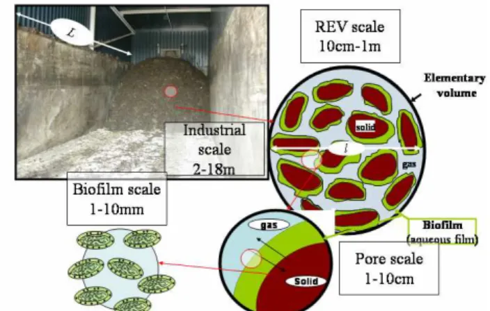
The process studied in our case consists in a closed reactor with positive aeration. In figure 1 on the upper left part, the geometry is briefly reminded. Air is distributed using several holes made in two veins. The homogeneity of the distribution is one of the key points, because if we need to provide microorganisms enough oxygen, we also have to avoid important drying which may block the reactive scheme. Under certain conditions (temperature and humidity), microorganisms cannot play their role and all the problem is to keep an equilibrium between temperature/water content/air distribution. The effects of humidity have particularly discussed in Pommier et al 2007. In figure 1, the different scales of the problem appear. If we have a look at the industrial scale, we can define a REV scale where an effective transport model can be derived from the transport processes in a detailed image of the porous medium so called the pore scale. The biofilm phase can also be homogenised because it appears as a porous medium and seeing it like an effective medium requires an averaging process made recently in Aspa et al. 2011.

Figure 1: Industrial composting process and the different scales associated, from the biofilm scale (1mm) to the industrial one (10m)

The other important point is the water content in the sludge and its prediction during composting. According to Richard et al. 2002, the moisture content must be controlled in order to maintain an efficient process. We will see this more in details further but in the reactive scheme, there is a high dependence upon the water content on the global reactivity. This could be interesting if we could follow humidity inside the wastes but it’s challenging because of the assumptions underlying the results of the measures we will have (how a large scale measurement could be a good indicator of the local water content?).

Thus, a macroscale model could give some indications and hopefully indicates how to optimize the process in term of aeration.

2. Methodology

We will recall the local scale equations, leading to the macroscale system fully coupled with biodegradation terms determined thanks to respirometric studies. In a last subsection, the parameter values missing in order to close the system will be explained.

2.1 Local scale model

At the pore scale, the set of governing equations are based on the basic fluid mechanics concepts. The medium is seen like a continuum; so, we can write the Navier Stokes equations in the gas phase (we supposed the fluid phase to be immobile) with a no slip condition upon the solid phase and the fluid phase.

For the mass transport equations, in the gas phase, classical convection and diffusion equations are used, with flux continuities on the interfaces between gas and liquid phase. For solid component, we only use classical ODE

forms, with an accumulation part and a reactive term. The heat transport is a convective conductive equation in the gas phase, and a conductive equation in the solid phase. Then, we average the whole set of equations to obtain the macroscale model. To do that, we use the classical theory and theorems of the volume averaging process and the reader could see some details in Puiggali & Quintard.1992. In our case, we will only present the final system.

2.2 Darcy’s scale model

Averaging all the equations over a REV, we can express a set of equations at the Darcy’s scale. The mass conservation for the gas phase is given by the continuity equation expressed like

(

)

2 2 2 g g

u

g

m

gsO

m

gsCO

m

gsH O

t

ρ

ε

∂

+ ∇ ⋅

ρ

=

+

+

∂

&

&

&

, where

ε

is the porosity,

ρ

g the gas density and

(

)

g g g g

K

u

p

ρ

g

µ

= −

⋅ ∇ −

is the intrinsic average velocity of the gas phase, given by the Darcy’s law. In equation 1,

2 gsH O

m

&

is the exchange term between the le gas and the immobile water phase.

2 gsO

m

&

and

2 gsCO

m

&

are the reactive terms corresponding respectively to O2 consumption and CO2 production. They are given by the following relations..

2 2 2 _{( )}X( ) ( ) (1 ) X( ) ) ( ) , ( 1 O b O sH opt O t b T f t M t MB K t MB C T Y Y R ×      ⋅ − ⋅ + + ⋅ ⋅ − =

µ

2 2 2 2 2 CO O O CO CO

M

M

R

P

R

=

⋅

⋅

In our case, we use the classical assumption that gas phase is ideal, so: ,

/ g i g g i g i P R T M ρ ∈ Ω =

∑

, where g P is the gas pressure, , g i

Ω the mass fraction of component I in the gas phase and

M

_iits molecular weight.

Gas species are transported in the gas phase and a general advection dispersion reaction equation is used.

(

)

.

gi g gi g gi gi g

u

g g

u

g gi g

D

gi

R

i

t

t

ρ

ερ

∂Ω

+ Ω

ε

∂

+ Ω ∇⋅

ρ

+

ρ

∇Ω + ∇⋅





ερ

∗

⋅∇Ω





= ±

∂

∂





, where i=CO2, O2, N2 (RN2=0). We

see that the dispersion transport appears in this equation. We have chosen to use a classical model defined like:

{

(

)

diffusive term dispersive term gi g g gi _{T g L T} g

D

u u

D

I

u

I

u

α

α

α

τ

∗





=

+



+

−











14444

4244444

3

, where

I

τ

is the tortuosity tensor for an isotropic medium.

L

α

represents the longitudinal dispersivity coefficient and

α

_T the transversal one. Water vapour transport is governed by one equation in the gas phase.

(

)

2 2 2 2 2 , , , g g H O gH O g g H O

u

g g

D

g H O

m

gsH O

t

ρ

ε

∂ Ω

+ ∇⋅

ρ

Ω

= ∇⋅





ερ

∗

⋅∇Ω





+

∂





&

But also, one in the solid phase:

(

)

2 2 2

1

s sH O

R

H O

m

sgH O

t

ρ

ε

∂ Ω

−

=

+

∂

&

Following Puiggali and Quintard 1992, we assume that the local equilibrium assumption is valid in our composting problem, so, no differences between an average value of solid humidity and the one in the gas exist. This imposes that the gas phase is at the equilibrium so that

2 , 2

gH O eq gH O

Ω

= Ω

. This allows us add the two preceding equations and to obtain the one we will now use.

(

)

2 2

(

)

2 2 2 2

1

s sH O

R

_{H O} g gH O _{g gH O}

u

_{g g}

D

gH O _{gH O}

t

t

ρ

ρ

ε

∂ Ω

ε

∂ Ω

ρ



ερ

∗



−

=

−

−∇⋅

Ω

+∇⋅



⋅∇Ω



∂

∂





We will calculate 2 2 , , i g g H O e q s a t H O i g i X M M ∈ Ω

Ω =

∑

assuming that at the equilibrium, we have

T

=

T

_sat, and

2 ,

H O eq sat

X

=

X

.

(

)

(

)

( )

₍

₎

₍

₎

₍

₎

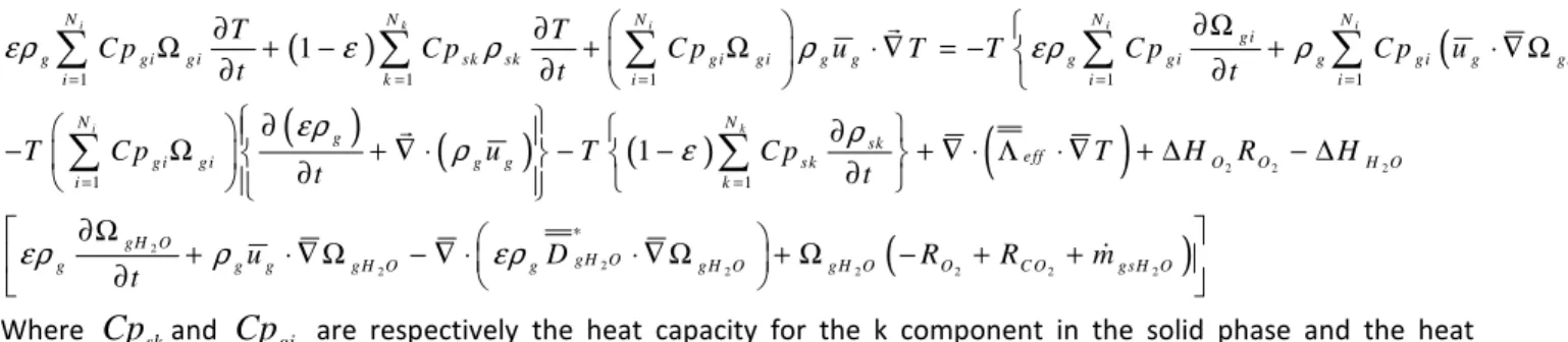
1 1 1 1 1 1 1 1 1 i k i i i i k N N N N N g i g gi g i sk sk g i gi g g g g i g g i g gi i k i i i N N g sk e ff g i g i g g sk i k T T C p C p C p u T T C p C p u t t t T C p u T C p T t t ερ ε ρ ρ ερ ρ ερ _ρ ρ ε = = = = = = = ∂Ω     ∂ ∂ Ω + − + Ω  ⋅ ∇ = −  + ⋅ ∇ Ω  ∂ ∂    ∂  _∂      _∂  −  Ω  _∂ + ∇ ⋅ −  − _∂ + ∇ ⋅ Λ ⋅ ∇ +     

∑

∑

∑

∑

∑

∑

∑

r r

(

)

2 2 2 2 2 2 2 2 2 2 2 O O H O gH O gH O g g g g H O g g H O g H O O C O gsH O H R H u D R R m t ερ ρ ερ ∗ ∆ − ∆ ∂Ω  _{ }  + ⋅ ∇ Ω − ∇ ⋅ ⋅ ∇ Ω + Ω − + +   ∂    & 

Where

Cp

_skand

Cp

_gi are respectively the heat capacity for the k component in the solid phase and the heat capacity for the i component in the gas phase. Finally, other reactive terms necessary in the biodegradation process are summarized in table 1 and the definitions and values of this biodegradation process are given in Table 3.

Table 1: biodegradation scheme

Micro-organisms growth kinetics

(

)

₍₎ X() ( ) X() ) ( , ) ( X 2 t bT t t MB K t MB C T dt t d B O sH ⋅ − ⋅ + ⋅ =

µ

Rapidly biodegradable consumption kinetics X() ) ( X ) ( ) ( X ) ( ) ( ) ( X ) ( ) ( ) , ( 1 ) ( 2 t t t MH K t t MH T K t t MB K t MB C T Y dt t dMB MH h b O sH + ⋅ + + ⋅ ⋅ − = µ Slowly biodegradable consumption kinetics X() ) ( X ) ( ) ( X ) ( ) ( ) ( t t t MH K t t MH T K dt t dMH MH h + ⋅ − = dry matter consumption MS MS O2

R

C

R

=

−

⋅

2.3 Parameters

Our model needs two types of parameters. Firstly, transport parameters must be specified and measured. Then, kinetic parameters must be estimated in order to be coupled with the transport problem. All of them are given in the next tables and the value used in our study case is given.

Table 2: Parameters appearing in the macroscale equations

Parameters notation Source Value Units

ε

Porosity Experiments (Druilhe et al.2008) 0.3 -

g

µ

dynamic viscosity in the gas phase Handbook of Chemistry and Physics 5

10

78

.

1

×

− kg/m/s

K Permeability Druilhe et al. (2008) 7

10

3

×

− 2

m

τ

tortuosity Kallel et al. (2004) 2 -

L

α

Longitudinal dispersion coefficient Experiment 0.4 m

T

α

Transversal dispersion coefficient - 0.2 m

2 molO

H

∆

Enthalpy of reaction O2 consumption Bailey and Ollis (1986) 5

10

3

×

J mol O

2 s

Λ

Solid thermal conductivity Trémier (2004) 0.5 W/m/K

Table 3: Values, sources and determination modes of biodegradation parameters.

Constant notation Source values Units

f Inter matter fraction 0.2 -

Y Rendement de production de biomasse 0.69 -

b

K

Half saturation constant for hydrolysable

matter

0.8 mol O2/m

3

MH

opt

a

_µ kinetic coefficient micro organism growth 5

10

27

.

1

×

−

s

−1

opt

b

_µ Optimum kinetic coefficient micro

organism growth 5

10

05

.

9

×

−

s

−1 opt

b

Optimal value for death micro-organisms 5

10

53

.

1

×

−

s

−1

hopt

k

Optimal kinetic for hydrolysis 5

10

56

.

2

×

−

s

−1

max Kmax bmax

T

_µ

=

T

=

T

Maximum temperature for growth

kinetics, hydrolysis and death

80 °C

min Kmin bmin

T

_µ

=

T

=

T

Minimum temperature for growth

kinetics, hydrolysis, and death

0 °C

opt Kopt bopt

T

_µ

=

T

=

T

Optimal temperature for growth kinetics,

hydrolysis, and death

40 °C 2 CO

P

Stoichiometric coefficient CO2 consumption 0.8 2 2 O CO

mol

mol

O H

P

2

Stoichiometric coefficient H2O production 1.5

2 2O O H

mol

mol

MS

C

Stoichiometric coefficient MS consumption 0.021 2 O MS

mol

mol

G(T) Temperature function Respirometric tests See after -

Using these coefficients, we can define non linear functions for the biodegradation scheme introduced in Trémier et al 2005. Let’s define G(T), it is a function depending from several parameters and especially from

max Kmax bmax

T

_µ

=

T

=

T

,

T

_µmin

=

T

_Kmin

=

T

_bmin,

T

_µopt

=

T

_Kopt

=

T

_bopt and can be written using a cardinal function (see Rosso et al 1995).

(

)(

)

(

) (

)(

) (

)(

)

2 m a x m in m in m in m ax m in ( ) 2 b b b op t b b o pt b bo p t b o p t b b o p t b T T T T G T T T T T T T T T T T T − − = _{ } − _ − − − − + − _ Firstly,

b T

( )

,

K

_h

( )

T

and

(

)

2

,

_{sH O}

T C

µ

that will be used in order to define respectively the dependence of micro organisms growth with temperature, the hydrolysis rate and biodegradable matter consumption can be written as:

( )

_opt

( )

b T

=

b

×

G T

,

K

_h

( )

T

=

k

_hopt

×

G T

( )

,

(

)

(

)

2 2 2 2 2 , _{sH O opt}ln _{sH O opt} gO ( ) gO gO C T C a C b G T K C µ ₌ µ ₋ µ _⋅   ₊

At this point, we clearly exhibit the high dependence with temperature for the biodegradation (from

G T

( )

) but also with water content with the

(

)

2

ln

opt sH O opt

a

µ

C

b

µ



₋







term. Stoechiometric coefficients

P

CO2,

P

H2O, and

C

MS

are determined empirically using the balance equation introduced in Trémier, 2004 O H y xCO O z y x O H C_{x y z 2 2 2} 2 2 4  → +     − + + .

In this section, biodegradation kinetics and transport parameters have been set. Reactive terms come also from an averaging process, because we measure the reactivity in a porous medium composed of several REV. Those represent a macroscale behaviour which have been coupled with the macro scale model presented. Determining the parameters missing by measurements, we are now able to use this numerical tool and try to check if it matches with experimental data.

3. Comparison between industrial scale experiments and simulations

In order to validate our model and to use it as an optimization tool for the industrial process, an experimental campaign was made during one month and some temperature recording and balances have been made for H2O and

dry matter. The temperature recording was presented in Henon et al. 2009, but the following figure 2 will summarize the locations of the recorders and dimensions. The first results obtained are given in figure 3.

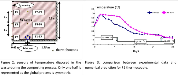
Figure 2: sensors of temperature disposed in the waste during the composting process. Only one half is represented as the global process is symmetric.

Figure 3: comparison between experimental data and numerical prediction for F5 thermocouple.

During the experiments, the aeration was supplied as follow: - Flow rate equal to Q1= 340m3/h during 9 days.

- Flow rate equal to Q2= 240m3/h during 16 days. - Flow rate equal to Q3= 600m3/h during 3 days.

No turning of the composting mixture has been made during this experiment in order to keep the sensors at their initial locations but also to be able to analyse the distribution of water without any perturbation due to mixing.

On Figure 3, we can see a good agreement, between predicted and measured values. In the middle part, we observe that the numerical model overestimates the temperature from the 3rd to the 18th day. Several over locations have been checked and the results look the same. At this step, we can explain these differences mainly by some heterogeneity in biomass concentration in the waste but also from the drying process which is not limited in our model. No sorption isotherm was added in order to limit the evaporation process. This is confirmed in table 4, H2O

losses are more important in our numerical case, but we represent fairly well the dry matter losses, and that confirms the good accuracy of our model compared to experimental data.

Table 4: Final balance for H2O and dry matter from the experiment compared to numerical simulation.

4. Optimization

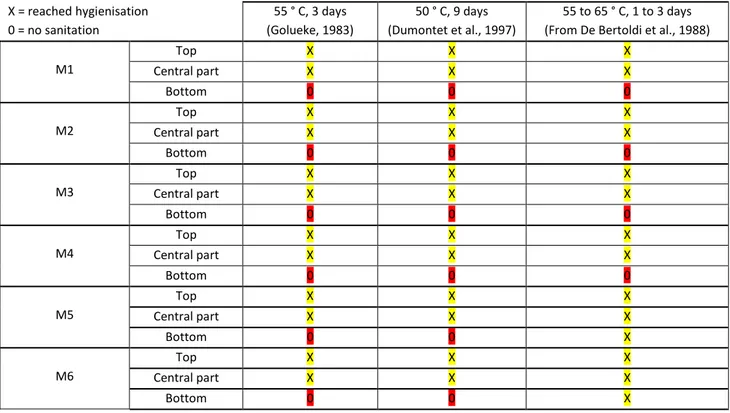
The above model was used to study several aeration protocols in order to find the best way to achieve sanitation process, i.e a temperature of 55°C maintained during 3 days according to Golueke 1983. Other couples temperature/time have been proposed by Dumontet et al. 1997 (50° during 9 days) or in De Bertoldi et al (55 to 65°C for 1 to 3 days). All the tests made are summarized in the table 5. We have simulated changes of the flow rate (240m3/h except in M2 which is the base case), the aeration (2 inlets in M5 & M6), heated the ground and air (M4 & M5) or simulated mixing (in M4 & M6). These are the model specifications:

- M1: Base case : flow rate constant equal to 240 m3 /h _{during all the process (28 days)}

- M2: Flow rate varying (like in the results presented before).

- M3: Identical to M1, with a mixing (15th day)

- M4: Ground and air heated at 30°C + mixing 15th day

- M5: Two inlets with constant flow rate (240 m3 /h) + ground and air heated at 30°C

- M6: Identical to M5, mixing 15th day.

Table 5: Results of the optimization tests with highlights on sanitation.

Hygienisation

Experimental balance Numerical balance

H2O losses (% of the initial mass) 72.1 93

Dry matter losses (% of the initial mass) 10.58 12.9

0.65 m 1.35 m

Wastes

F7-F9 F8 F4-F6 F5 F1-F3 F2 1 m 1 m Symmetry Inlet vent 2.5 m 0 10 20 30 40 50 60 70 80 0 1 2 3 4 5 6 7 8 9 10 11 12 13 14 15 16 17 18 19 20 21 22 23 24 25 26 27 28 Jours Te m pé rat ur e F5 expé F5 num Q=340m3/h Q=240m3/h Q=600m3/h 0 10 20 30 40 50 60 70 80 0 7 14 21 28 Days Temperature (°C) F5 Exp F5 num Q1=3403 _/h Q=240 3 _/h Q=600 3 _/h thermoboutons

X = reached hygienisation 0 = no sanitation 55 ° C, 3 days (Golueke, 1983) 50 ° C, 9 days (Dumontet et al., 1997) 55 to 65 ° C, 1 to 3 days (From De Bertoldi et al., 1988)

Top X X X Central part X X X M1 Bottom 0 0 0 Top X X X Central part X X X M2 Bottom 0 0 0 Top X X X Central part X X X M3 Bottom 0 0 0 Top X X X Central part X X X M4 Bottom 0 0 0 Top X X X Central part X X X M5 Bottom 0 0 X Top X X X Central part X X X M6 Bottom 0 0 X

All the tests without any mixing (M1, M2, and M5) give the same results from the sanitation point of view. Only the upper and central part of the whole domain can reach the temperature of 55°C during more than 3 days. In the M5 and M6 cases, another part of the domain can be sanitized but according to De Bertoldi et al., 1988. One way to achieve this goal is to mix the wastes and to put the upper part in the bottom for the last period of the composting process. The final balances give the following results. The mixing effects are mainly a less important drying, but it is not sensible as we estimate a global balance. For dry matter, no important differences can be seen.

Table 6 : H2O and dry matter balances over the different optimization tests

M1 M2 M3 M4 M5 M6

H2O losses(% initial mass) 64.5 69.5 63 64 65.5 64

Dry matter losses (% initial mass) 20.5 21 21 20 20 20

But, if we make a close-up on water content, at the end, after 28 days composting, the differences appear clearly. Due to mixing, H2O is more homogeneous in the waste and it seems that no limitation due to insufficient

water content exists. Two inlets homogenise air flux and consequently the water content inside the waste.

Figure 4: Comparison of apparent volumetric mass H2O fields for from letf to right M1 and M3 (M1 +mixing) and M5

and M6 (M5 + mixing). Water content is maximum in red and equal to zero in dark blue.

5. Conclusion

We have presented a new model of reactive transport in porous media where biological reactions take place. This is developed at the so called Darcy’s scale, i.e, a scale where the influence of the porous medium appears in effective coefficients. This model takes into account several couplings, drying and also a biological model.

After a validation test by comparing the results given by the model to the one obtained during an experimental campaign, we have used this to test several situations in order to optimize the sanitation process but also the dry matter consumption and H20 evaporation. It appears that it seems necessary to mix the waste once

during the process in order to ensure that all the porous medium reach the sanitation criteria, except in one case, injecting the same flow rate using two inlets and maintaining the ground and incoming air inside the waste at 30°C. So getting back the heat from the outlet to preheat the incoming air could allow, in some cases, to reach the sanitation criterion.

The next step in our case will be to take into account the evolutions of transport parameters and to validate our model on several wastes using pilot experiments. This has begun and several input data are now available from Huet et al. 2012. He has shown some important variations on porosity and permeability inside the waste during the composting process. Taking that into account could allow us to have a more accurate model.

References

- Pommier, S., Chenu, D., Quintard, M., Lefebvre, X. (2007). A logistic model for the prediction of the influence of water on the solid waste methanisation in landfills. Biotechnology and Bioengineering, 97, 473-482.

- Trémier A., De Guardia A. and Massiani C.., Paul E., Martel J.L., (2005). A respirometric method for characterizing the organic composition and biodegradation kinetics and the temperature influence on the biodegradation kinetics, for a mixture of sludge and bulking agent to be co-composted. Bioresource Technology. 2005, vol.96, n°2, p.169-180.

- Hénon F.,(2008) Caractérisation et modélisation des écoulements gazeux au cours du compostage de déchets organiques en taille réelle, Thèse de l’Université de Rennes.

- Pujol A., Debenest G., Pommier S., Quintard M. & Chenu D. (2011): Modeling Composting Processes with Local Equilibrium and Local Non-Equilibrium Approaches for Water Exchange Terms, Drying Technology, 29:16, 1941-1953

- Hénon F., Trémier A., Debenest G., Martel J-L., Quintard M. (2009) A method to characterize the influence of air distribution on the composting treatment: monitoring of the thermal fields. Global NEST J., 11. pp. 172-180. ISSN 1008-4006 - Golueke C. G. (1983). Decision and strategies for regional resources recovery. In Biological reclamation and land utilisation of urban wastes, Napoli, 310-313

- Aspa Y., Debenest G., Quintard M. Effective dispersion in channeled biofilms. Int J Environ Waste Management. 2011; 7(1-2): 112-131.

- Richard,T.L.; Hamelers, H.V.M.(Bert); Veeken, A.; Silva, T.(2002) Moisture relationships in composting processes. Compost Science & Utilization, 10(4), 286–302.

- Puiggali, J.R.; Quintard, M. Properties and simplifying assumptions for classical drying models. In Advances in Drying; Mujumdar, A.S., Ed.; Hemisphere Publishing Corporation: New York, 1992; 109–143.

- Druilhe, C., Benoist, J. C., Radigois, P., Teglia, C., Trémier, A. (2008). Sludge composting : Influence of the waste physical

preparation on initial free air space, air permeability and specific surface. ORBIT2008, Wageningen, The Netherlands.

-CRC Handbook of Chemistry and Physics. 85th ed. CRC Press: Boca Raton, FL, 2004-2005; p 3-522, 9917

-Kallel, A., Takana, N., and Matsuto, T. (2004). Gas permeability and tortuosity for packed layers of processed municipal

solide waste and incinerator residue. Waste Management and Research, 22 :186-194.

- Bailey, J., Ollis, D. (1986). Biochemical engineering fundamentals. McGraw – Hill Book Co, Singapore.

- Trémier, A. (2004). Modélisation d'un traitement par compostage. Développement d'outils expérimentaux d'étude du

procédé et conception du modèle. 2004, Thèse de l'Université de Provence. p. 274.

- Rosso,L., Lobry,J.R., Bajard,S.,and Flandrois, J.-P.(1995).Convenient model to describe the combined effects of temperature and phonmicrobial growth. Applied and Environmental Microbiology, 61:610–616.

- Dumontet S., Dinel A., Baloda S. (1997). Pathogen reduction in biosolids by composting and other biological treatments: A

litterature review. In International congress. Maratea 10-13 october 1997, 251-295.

- De Bertoldi M., Zucconi F., Civilini M. (1988). Temperature, pathogen control and product quality. BioCycle, 29, 2: 43-47 - Huet J. , Druilhe C., Trémier A., Benoist J-C., Debenest G., (2012) the impact of compaction, moisture content, particle size and type of bulking agent on initial physical properties of sludge-bulking agent mixtures before composting. Bioresource Technology, dx.doi.org/10.1016/j.biortech.2012.03.031.