Construction of bootstrap confidence intervals on sensitivity indices computed by polynomial chaos expansion

This is an author-deposited version published in:

http://oatao.univ-toulouse.fr/

Eprints ID: 9717

To link to this article: DOI: 10.1016/j.ress.2013.09.011

URL:

http://dx.doi.org/10.1016/j.ress.2013.09.011

To cite this version:

Dubreuil, Sylvain and Berveiller , Marc and Petitjean,

Frank and Salaün, Michel Construction of bootstrap confidence intervals

on sensitivity indices computed by polynomial chaos expansion. (2014)

Reliability Engineering & System Safety, vol. 121 . pp. 263-275. ISSN

0951-8320

O

pen

A

rchive

T

oulouse

A

rchive

O

uverte (

OATAO

)

OATAO is an open access repository that collects the work of Toulouse researchers and

makes it freely available over the web where possible.

Any correspondence concerning this service should be sent to the repository

administrator:

[email protected]

Construction of bootstrap confidence intervals on sensitivity indices

computed by polynomial chaos expansion

S. Dubreuil

a,b,n

, M. Berveiller

c

, F. Petitjean

b

, M. Salaün

a

a_{Institut Clément Ader (ICA), ISAE, F-31055 Toulouse, France} b_{Institut Catholique d'Arts et Métiers (ICAM), F-31300 Toulouse, France}

c_{EDF R&D-Département MMC, Site des Renardières, F-77818 Moret-sur-Loing, France}

a r t i c l e

i n f o

Keywords: Sensitivity analysis Polynomial chaos expansion Bootstrap re-sampling

a b s t r a c t

Sensitivity analysis aims at quantifying influence of input parameters dispersion on the output dispersion of a numerical model. When the model evaluation is time consuming, the computation of Sobol' indices based on Monte Carlo method is not applicable and a surrogate model has to be used. Among all approximation methods, polynomial chaos expansion is one of the most efficient to calculate variance-based sensitivity indices. Indeed, their computation is analytically derived from the expansion coefficients but without error estimators of the meta-model approximation. In order to evaluate the reliability of these indices, we propose to build confidence intervals by bootstrap re-sampling on the experimental design used to estimate the polynomial chaos approximation. Since the evaluation of the sensitivity indices is obtained with confidence intervals, it is possible to find a design of experiments allowing the computation of sensitivity indices with a given accuracy.

1. Introduction

Performing global sensitivity analysis is often a major step in uncertainties propagation studies. It helps to understand how uncertainties of a quantity of interest could be explained and reduced. Different types of sensitivity analysis can be performed (see[21]). This paper focuses on variance-based ones, computed by polynomial chaos expansion. Sensitivity indices, coming from variance decomposition (ANOVA), are relevant informations as they allow one to quantify effect of a variable (alone or in inter-action with one or more variables) but require estimate of many partial variances (see[21]for a description of sensitivity indices). When these partial variances cannot be expressed analytically, which is often the case in industrial applications, a Monte Carlo based method, developed in [23], leads to an approximation of these indices. If the computation of the model is time consuming (finite element models for example), Monte Carlo simulations become unrealistic and a common way to tackle this problem is the use of a meta-model. In this case, the idea is to replace the true model by an analytical one as precise as possible and then to use it in the Monte Carlo methodology. This involves two types of error: a meta-modelling error coming from the difference between the

true model and its approximation and a sampling error due to the Monte Carlo methodology, used for the sensitivity indices computation.

An efficient way to compute sensitivity indices is to use an approximation of the model by polynomial chaos expansions (PCEs). Indeed,[26]shows that sensitivity indices are analytically calculated with the coefficients of that expansion. Then, the two types of error, given earlier, are reduced to the meta-modelling error only. Hence, it is of great importance to quantify and control it. The quality of meta-models is usually defined as the difference between the true model and the meta-model. This difference can be expressed using several error criteria like coefficient of deter-mination, Mallows Cp, cross-validation, etc. Numerous methods propose iterative constructions of meta-models based on one (or several) of these criteria. For example, in[20], a quadratic surface response is built based, first, on the minimization of the sum of squared error, then in four different error criteria (Mallows Cp, AIC, BIC, adjusted coefficient of determination) and finally on leave-one-out validation. Concerning sensitivity analysis,[4]proposes an innovative construction of sparse PCE and selects the best PCE thanks to a corrected leave-one-out error. All these methodologies are efficient but do not take into account the aim of the meta-model. Moreover, it is difficult to link a global criterion error to the error on sensitivity indices computed from the meta-model. Finally, it is difficult to target a global error criterion value that allows a level of confidence on sensitivity indices. This problem also arises in reliability analysis and many authors propose error measurements and adaptive algorithms based on the probability

n

Corresponding author at: Institut Clément Ader (ICA), ISAE, F-31055 Toulouse, France. Tel.: þ33 561339245.

E-mail addresses:[email protected] (S. Dubreuil),[email protected] (M. Berveiller),[email protected] (F. Petitjean),[email protected] (M. Salaün).

of failure obtained by models and not only on global meta-modelling error. For example, in[11], the authors use a complete quadratic response surface as a meta-model and build confidence intervals by Jack-knife re-sampling around the design point. In

[16], a bootstrap re-sampling on the failure probability is used to construct an optimized PCE. Confidence interval constructed by bootstrap re-sampling is also widely used in global sensitivity analysis. Plischke et al. [17] use bias-reducing bootstrap on variance-based and density-based sensitivity indices computed by sampling. Castaings et al.[5]use bootstrap on density-based sensitivity indices computed by different sampling strategies. In the field of sensitivity analysis performed by meta-models,[13]

uses reduced-basis meta-models to estimate variance-based sen-sitivity indices and combine the property of reduced-basis meta-model and bootstrap re-sampling to compute confidence intervals. Storlie et al.[25]compares several types of meta-models and also uses bootstrap re-sampling on this meta-models to obtain con-fidence intervals.

This paper proposes to take advantage of the PCE in the estimation of variance based sensitivity indices. Then, in order to know if this approximation is accurate enough to estimate partial variances, a way to construct confidence intervals by bootstrap re-sampling is presented. In the first part of this paper, some important features about PCE and the determination of sensitivity indices are recalled. One important point deals with the method used to construct the polynomial basis. A quite recent methodol-ogy based on the Least Angle Regression (LAR) algorithm and developed in[3]is used. The second part presents an application of bootstrap re-sampling [10] to the computation of sensitivity indices, when they are estimated by PCE. Some results about the determination of confidence intervals are recalled and an algo-rithm is presented which is set up to build a design of experiments allowing one to obtain sensitivity indices with a given level of confidence. Finally, this methodology is tested, first, on academic cases (Ishigami and g-Sobol' functions) and, second, is used for a sensitivity analysis on a finite element model of satellite TARANIS, designed by the Centre National d'Etudes Spatiales (France).

2. Determination of sensitivity indices by polynomial chaos expansion

2.1. Approximation of a stochastic model by a PCE

Let us consider a numerical model yðXÞ, that depends on a random vector X ¼ fX1;…; Xng of n independent random variables, defined by the joint probability density function (PDF), say fXðxÞ ¼∏ni ¼ 1fXiðxiÞ. It is shown[24]that any second-order random

variable can be expanded into a polynomial decomposition as yðXÞ ¼ ∑1

i ¼ 0

Ci

ϕ

iðX1;…; XnÞ ð1Þ where f

ϕ

igi A N is an adequate orthogonal polynomial basis, with respect to the joint PDF, and fCigi A Nare unknown coefficients. In practice, decomposition Eq.(1)is truncated to a finite number of terms, say P, according to

yðXÞ ( byðXÞ ¼ ∑P ) 1 i ¼ 0 C_i

ϕ

_iðX1;…; XnÞ ¼ ∑ P ) 1 i ¼ 0 C_i

ϕ

_iðXÞ ð2Þ This paper only deals with the so called non-intrusive methods which do not need a modification of the numerical code comput-ing the output Y. They are simple to implement and do not ask special form of Y, except that E½Y2_{+ o 1.}

The next subsections present the construction of a basis

ϕ

i " # and the computation of the coefficients Ci.

2.2. Construction of the candidate basis

It is shown in[27] that classical univariate polynomial bases should be used for usual distributions (see Table 1). Then the orthogonal multivariate polynomial basis is obtained from the product of each univariate polynomial. This approach is chosen because only usual distributions are used. In other cases, the simplest solution consists in an iso-probabilistic transformation of the input variables into standard normal ones[14].

The multivariate polynomial basis in Eq.(1)is composed of an infinity of terms. As seen in Eq.(2), this basis is truncated to a finite number of terms, say P. In the following, polynomials are ranked by order (first polynomials are univariate of degree one, then multivariate using two variables of degree one, then the univariate at degree two, etc.).

The simplest way to truncate the basis is then to choose the P first polynomials. For example, the number P of polynomials necessary to reach a maximal order p is P ¼ ðn þpÞ!=ðn!p!Þ, where n is the number of random variables. This strategy is efficient for problems of small dimension and responses that can be approxi-mated by low degree polynomials. When it is not the case, the number of terms becomes important and leads to conditioning problems. Considering this issue, considerable research efforts were done during the last years to create efficient selection algorithms, leading to sparse bases in regression area and parti-cularly in PCE area[2]. They will be detailed inSection 2.3.2. 2.3. Computation of the coefficients

2.3.1. Ordinary least square

Coefficients Ci are determined by minimizing the quadratic

norm of the error ɛy¼ Y )

Φ

C, between some exact values yðXÞ estimated at N different points (experimental design of size N) concatenated into vector Y, and their estimation by the truncated polynomial expansion, concatenated into vector

Φ

C, where C is the vector of unknown coefficients Ciin Eq.(2)and

Φ

AMN;Pis the matrix of regressors. Column vectors of matrix

Φ

are evaluations of polynomials

ϕ

i, i A½0; P )1+, at the N points of the experimental design. The least-square minimization criterion leads to

C ¼ ð

Φ

t

Φ

Þ) 1

Φ

tY: ð3Þ

2.3.2. LAR

Let us now introduce classical notations for sparse basis. First, the multi-index is

α

¼ f

α

1⋯

α

i⋯

α

ng, and A is the family of multi-indices

α

. From now, polynomial

ϕ

_αis the one acting on variables

Xiat power

α

i, for i A½1; n+. Its total degree is j

α

j ¼∑n

i ¼ 1

α

i. With such notations, the polynomial chaos expansion of a stochastic model yðXÞ (see Eq.(2)) reads

yðXÞ ( byðXÞ ¼ ∑ αAA

Cα

ϕ

αðXÞ: ð4Þ

Given a full candidate basis B of maximal degree p, with p ¼ maxj

α

j and cardðBÞ ¼ ðn þ pÞ!=ðn!p!Þ, a polynomial chaos

expan-sion is said sparse if cardðAÞ o cardðBÞ. As the expanexpan-sion coeffi-cients are determined by regression, several tools, initially set-up

Table 1

Univariate orthogonal polynomials for usual ran-dom variables.

Random variable Orthogonal polynomials

Gaussian Hermite Uniform Legendre

Beta Jacobi

in this area, can be used to select relevant polynomials. In this study, we shall use the Least Angle Regression (LAR) algorithm, introduced in [9], and already used in [1] to polynomial basis selection. Let us now recall some important features of this algorithm. First of all, the LAR returns a collection of meta-models that are less and less sparse (the last iteration is the classical least-square solution) in cardðBÞ iterations. The meta-model, which is selected in this collection, is determined by estimation of a given indicator. This point will be discussed later on. So the LAR algorithm proceeds as follows:

-

_{Set all coefficients C}αto 0.

-

Find the polynomial that is the most correlated with the response, say

ϕ

j1.

-

Take the largest possible step in the direction of

ϕ

j1 until

another polynomial, say

ϕ

_j2, has as much correlation with the current residual.

-

_{Define the equiangular direction between}

ϕ

j1and

ϕ

j2and take

the largest step in this direction, until a new predictor has as much correlation with the residual, and so on.

Note that, in[1], the LAR is only used for variable selection and coefficients Cα are calculated by least-square method for each sparse basis.

Here, once the LAR algorithm returned the P meta-models, one has to choose the best one according to an error criterion. Several regression error measurements have been tested in the literature, see for example[3] and the discussion in [9]. We recall two of them, used in next sections: the classical coefficient of determina-tion R2_{and the leave-one-out error Q}2_.

2.4. Regression error measurement 2.4.1. Coefficient of determination R2

The coefficient of determination is defined as R2_{¼ 1 )}∑Ni ¼ 1ðyi)ybiÞ2

∑N

i ¼ 1ðyi) yÞ2 ;

where yiand byi are respectively evaluations of the real model and of the meta-model at points xi, while

y ¼1 N ∑

N

i ¼ 1 y_i:

This coefficient measures the generalization error, i.e. the part of variance of the real model explained by the meta-model [6]. A major drawback of this coefficient is that it only takes into account the points of the experimental design. Moreover, it tends to one when the number of polynomials in the meta-model increases, which makes it irrelevant to find over-fitting phenomena. To take into account the number of terms in the meta-model, other indicators are available, for example Mallows's Cp[15].

Considering these drawbacks, coefficient R2_{has to be used with}

care and its value has to be compared with other indicators that are less sensitive to over-fitting, e.g. the leave-one-out error.

2.4.2. Leave-one-out error

Leave-one-out is a particular case of cross-validation, where the size of validation set is one. The idea is to leave one point out of the design of experiments, to create a meta-model on this new design, then to evaluate the residual at the left point and, finally, to loop on each point of the original design of experiments. This methodology can be quantified through the following formula, where byð ) iÞstands for the value at xi of the meta-model built on

the experimental design in which point xihas been removed Q2¼ 1 )∑ N i ¼ 1ðyi)by ð ) iÞ Þ ∑N i ¼ 1ðyi) yÞ2 : As for the R2

coefficient, the leave-one-out coefficient can be penalized by the number of terms in the meta-model. Such a penalized Q2_{is used for the selection of the meta-model within}

the collection obtained by the LAR algorithm (see [3] for more details).

2.5. Construction of the design of experiments

The construction of an experimental design consists in choos-ing a method to sample in the space of input variables in order to compute the N exact values yðXÞ used in the least-square problem. In our study, we mainly used Monte Carlo sampling which is a random sampling in the joint PDF of the input variables. A comparison with Latin Hypercube Sampling (LHS) is performed

Section 4.1.3. LHS design of experiments splits the input space into equiproportional subspaces and allows only one sample per sub-space which leads to a better filling of the sub-space.

2.6. Post processing 2.6.1. Statistical moments

Once the PCE is built (i.e. once the basis is chosen and the coefficients are computed) statistical moments are computed analytically. As the decomposition functions

ϕ

αhave nice proper-ties of orthogonality and zero mean, it can be shown (see[26]) that E½byðXÞ+ ¼ C0; and Var½byðXÞ+ ¼ ∑ αAA C2αE½

ϕ

2 αðXÞ+: 2.6.2. Sensitivity analysis

The idea, pointed out in [26], is to identify the polynomial chaos expansion with an ANOVA decomposition (see [18] for example). For this purpose, Eq.(4)is rewritten according to b yðXÞ ¼ y₀þ ∑N i ¼ 1 ∑ αALi Cα

ϕ

αðXiÞ þ ∑ N ) 1 i1¼ 1 ∑N i2¼ i1þ 1 ∑ αAL_i1;i2 Cα

ϕ

αðXi1; Xi2Þ þ⋯ þ ∑ N ) s þ 1 i1¼ 1 ⋯ ∑ N is¼ is ) 1þ 1 ∑ αAL_i1;…;is

Cα

ϕ

αðXi1;…; Xi

sÞ

þ⋯ þ ∑ αAL1;…;N

Cα

ϕ

αðX1;…; XNÞ; ð5Þ where Li1;…;isrepresent sets

Li1;…;is¼

α

¼ ð

α

kÞk ¼ 1;…;n

α

kANn; k A ði₁;…; isÞ

α

k¼ 0; k =2 ði1;…; isÞ : , ) : (

Then the identification with the ANOVA decomposition is straight-forward. Moreover, sensitivity indices, or Sobol' indices [22], derived from this decomposition, can be computed with coeffi-cients of the sparse polynomial chaos decomposition[4], b Si1;…;is¼ ∑αAL i1;…;is C2αE½

ϕ

2 αðXi1;…; Xi sÞ+ Var½byðXÞ+ : ð6Þ

The most common sensitivity indices are the first order ones and the total ones. The first order sensitivity index of variable Xi, called

Si, gives the part of the output variance explained by the

its approximation reads b S_i¼∑αAL_iC 2 αE½

ϕ

2 αðXiÞ+ Var½byðXÞ+ :

Total sensitivity indices of an input variable Xi, called STi, takes into

account all interactions between Xi and all other variables. Its

estimate by polynomial chaos expansion is given by b STi¼ ∑αALþ i C 2 αE½

ϕ

2 αðXiÞ+ Var½byðXÞ+ ; where Lþ

i is the set Liþ¼"

α

AA=

α

ia0#. Let us remark that, according to Eqs. (5) and (6), if there is no interaction in the model, the sum of first order indices is one and total index STiis

equal to first order index Sifor every variable Xi.

This section shows how the quality of sensitivity indices is linked to the quality of the approximation by the meta-model. Nevertheless, accuracy needed for sensitivity analysis is strongly dependent on its aim (variable selection, variable ranking, variance reduction). So it seems difficult to use a global quality criterion (like R2 _{or Q}2 _{described before) to reach the level of accuracy}

needed for sensitivity analysis. For example, in[4], the authors propose to target Q2A½0:990; 0:999+ to have a correct approxima-tion of sensitivity indices. In order to have a goal-oriented information, we propose here to use bootstrap re-sampling on the design of experiments to build confidence intervals on sensitivity indices approximated by PCE.

3. Bootstrap re-sampling applied to polynomial chaos expansion

3.1. Construction of confidence intervals by bootstrap re-sampling Bootstrap [10]is a re-sampling method which aims at deter-mining confidence intervals on a quantity of interest using only one design of experiments. It is well suited when the computation of this quantity is time-consuming and use of replicates is then impossible. The main idea is to create several new designs of experiments, say B, by drawing with replacement in the first one (source design) and, then, to use these new designs to get an empirical distribution of the statistic variables calculated on these designs. This methodology has already been applied on several surrogate models, as in[13,11].

Here, we are interested in sensitivity indices, denoted as collec-tion S. PCE of the response of interest gives an estimator of these indices, denoted as bS. For every new design Dk (k ¼ 1;…; B), the methodology of sparse PCE described inSection 2is used, leading to sensitivity indices collections bSkfor design Dk(it should be noted that

in order to avoid ill-conditioning of regression matrix

Φ

defined in Eq.(3), the size of the design of experiments is three times higher than cardðAÞ, see [19]). After the computation of the B sensitivity indices collections (one per re-sampled design), empirical confidence intervals are built. Let bSn_i and VarbSi be the estimators of the mean and variance of the empirical distribution of the B collections of indices bS_ik. Different types of confidence intervals can be obtained from bootstrap re-sampling.

-

The first one is called standard interval, Si7u½1 )α=2+

ffiffiffiffiffiffiffiffiffiffiffiffi VarbSi q

; i A½1;…; n+;

where u½1 )α=2+is the 1)

α

=2 quantile of the standard normal distribution. This confidence interval is based on an asymptotic approximation of the bootstrap distribution by a normal one.

-

_{The second one is the percentile bootstrap. Confidence interval is}

b

Si½α=2+rSirbSi½1 )α=2+; i A½1;…; n+;

where bSi½α=2+ and bSi½1 )α=2+ are the

α

=2 and 1 )

α

=2 empirical quantiles.

This interval does not need any hypothesis on bS_i distribution, but needs a lot of re-sampling B (higher than 500, see[16]) in order to approximate these quantiles with a sufficient precision. The setting of this parameter is going to be discussed inSection 4.

-

The last one is the bias corrected and accelerated bootstrap (BCa), as first introduced in[8]. The main idea is to assume that

normality of the bootstrap distribution can be achieved by some transformation. In the following we only describe the construction of the intervals. For details on the theoretical basis, the reader is referred to[8]and also to[7]for a review on bootstrap confidence intervals. BCaconfidence intervals are

b

Si½α1+rSirbSi½α2+; i A½1;…; n+;

where bSi½α1+ and bSi½α2+ are the

α

1 and

α

2 empirical quantiles of

the bootstrap distribution.

α

1and

α

2are defined by

α

1¼

Φ

u0þ u0þ uα=2 1) aðu0þ uα=2Þ ) * and

α

2¼

Φ

u0þ u0þ u1 )α=2 1) aðu0þ u1 )α=2Þ ) *

where

Φ

is the standard normal cumulative distribution function, uα=2¼

Φ

) 1ð

α

=2Þ and u1 )α=2¼

Φ

) 1ð1 )

α

=2Þ. u0is called the

bias-correction and it is defined by u0¼

Φ

) 1ðcardðbSikobS_iÞÞ; k A ½1; B+. a is called the acceleration and it is linked to an idealized transformation of the bootstrap distribution to normality. This parameter is not known in practice but it is shown in [8]that a correct approximation of a is a ( ba ¼ ∑ N j ¼ 1ðbSiðÞ) bSi ) jÞ3 6f∑N j ¼ 1ðbSiðÞ) bSi ) jÞ2g 3=2 ð7Þ

where bSi ) j is the estimation of Si removing the jth point of the design of experiments, and bSiðÞis the mean of the N bSi ) jvalues. This interval is supposed to be more accurate as it takes into account some characteristic of the empirical distribution. It should be noted that it is a correction of the percentile bootstrap. Indeed if the correction terms u0 and a are null, then BCa is equal to

percentile bootstrap.

In the following numerical examples, we mainly used percen-tile bootstrap. BCaprocedure is illustrated but it should be noted

that the computation of the acceleration is time consuming. Hypothesis of normality for standard interval is too restrictive and never verified in practice. This is the reason why we will not use this one.

Considering informations given by these confidence intervals, we now propose a sequential strategy to create a design of experiments which eventually provides a required accuracy on the sensitivity indices.

3.2. Sequential construction of an optimized design of experiments Here an application of bootstrap re-sampling is presented in order to minimize the number of points in the design of experi-ments, so as to get sensitivity indices from PCE with a fixed level of confidence. The algorithm described here is inspired from a previous work[16], using bootstrap re-sampling in a similar way on reliability indices. Our methodology, summarized inFig. 1, is split in five main steps:

1. An experimental design of size N is used to build a polynomial chaos meta-model. Parameters for PCE construction are the degree p of the candidate basis B and the maximal size of the polynomial basis selected by the LAR algorithm, i.e. cardðAÞr N=3. Note that this last condition is due to the sparse nature of the selected meta-model. This can be adjusted according to the penalization coeffi-cient applied to leave-one-out error Q2_{, used in selection process.}

In our studies, during bootstrap re-sampling, all the PCEs are sparse enough to reach this condition. If it is not the case, one can increase the penalization coefficient. At first iteration, N is initi-alized by the user as well as the estimation pestof p.

2. B bootstrapped samples are used to construct the 95% con-fidence intervals (CIs) as presented in the previous section. This number B depends on the complexity of the response. Discus-sion about the choice of this parameter is presented later on. Three different confidence intervals being described inSection 3.1, the difference between them will be also discussed. 3. As far as convergence criterion is concerned, we choose to stop

the algorithm at the iteration for which all CIs sizes have reached a given range ½bSi½α=2+; bSi½1 )α=2++ for

α

¼ 0:05, which is formulated as a function of the maximum mean value of sensitivity indices (let us recall that, if there is no interaction, the sum of the first order sensitivity indices is equal to one). Once again, this convergence criterion will be discussed in the next section. 4. If the convergence criterion is not reached, naddnew points are

added to the experimental design and a new iteration starts. The value of naddis a compromise between the computation time of

a single model evaluation and the computation time of one algorithm iteration (B PCE constructions). If nadd is too small,

most of the time is spent during bootstrap iteration. If it is too large, the algorithm converges in less iterations but the final experimental design could be far from an optimal one. If the convergence criterion is reached, one obtains sensitivity indices with enough confidence, using an optimal experimental design. Sampling schemes that can be used to build and increase the experimental design are discussed in the following.

5. The last point deals with degree p of the candidate basis B. If it is too low, the convergence will never be reached and, if it is too high, cardðBÞ is large which makes the LAR algorithm time consuming. A way to increase it, if necessary, is described in the next section.

In conclusion this strategy leads to a PCE allowing to compute sensitivity indices with a given accuracy. It should be noted that this algorithm relies on the fact that PCE converges to the quantity of interest when the number of polynomials in the expansion and the degree of the candidate basis increase.

4. Numerical examples

This section discusses the choice of parameters in the method presented above. Let us first recall that these parameters are:

-

The number of bootstrap samples B.

-

The methodology used to create the design of experiments and to increase its size.

-

The degree p of the full candidate polynomial basis B and, possibly, the way to increase it.

-

_{The type of confidence interval (BC}aor percentile bootstrap).

-

The convergence criterion based on the confidence intervals size. All these points are enlightened through the example of the Ishigami function.

4.1. Application to Ishigami function 4.1.1. Presentation

The Ishigami function [21] is a well-known test case for sensitivity analysis because, among its three parameters, two have close first order sensitivity indices and one appears only in interaction. It is defined by

Y ¼ sin X1þ 7 sin2X2þ 0:1X43 sin X1;

where variables Xj have uniform distribution over the range

½ )

π

; þ

π

+. Sensitivity indices may be computed analytically as presented inTable 2.

In the following, all results are obtained by the methodology presented inSection 3.2.

4.1.2. Number of bootstrap samples B

Here, our goal is to check classical recommendation on the number of bootstrap samples B. Usually, building a 95% confidence interval by percentile bootstrap or BCarequires between 500 and

1000 bootstrap re-sampling [10]. As BCa is only a correction of

percentile bootstrap, all the following CI are constructed by percentile bootstrap. In order to fix the size of re-sampling, we propose to increase it from 100 to 1000 and to observe the variation of the lower and upper sensitivity indices CI boundaries for

α

¼ 0:05. This is performed using a sparse PCE of the function with a full candidate basis B of degree p¼ 10.

Fig. 2shows the evolution of bSX1½0:05=2+ (first order sensitivity

index of variable X1, lower CI boundary), and Fig. 3 shows

b

SX1½1 ) 0:05=2+(the upper CI boundary). In both cases, a comparison

is made for several sizes of design of experiments. Fig. 1. Sequential construction of the experimental design leading to sensitivity

indices with a fixed level of confidence.

Table 2

Ishigami function—sensitivity indices. Variable Analytical values

Si STi

X1 0.3138 0.5574

X2 0.4424 0.4424

Such a comparison was done for the three variables and the same two conclusions can be drawn:

1. The bigger the design of experiments is, the faster is the convergence as a function of B. This allows one to be confident in the fact that number B can be fixed, in a conservative way, at the first iteration.

2. Even for small design of experiments sizes, an admissible convergence in B is reached as soon as B¼700. So, this value will be kept in the following.

4.1.3. Choice of the methodology to create the design of experiments As an iterative algorithm is proposed to increase the experi-mental design, the position of the samples in the input variables space has to be discussed. Several experimental design strategies are possible namely Monte Carlo sampling (random sampling using the joint PDF of the input variables) or Latin hypercube sampling (LHS).

Bootstrap re-sampling is usually performed on random experi-ments. Nevertheless, the next section gives a comparison between

results obtained with a Monte Carlo design of experiments and a LHS one. In this last case, note that a new LHS experimental design is built at each iteration. Like in the previous section, sensitivity indices are obtained by sparse polynomial chaos expansion with a full candidate basis of degree p¼10 and confidence intervals are built with 700 bootstrap repetitions with percentile bootstrap method.

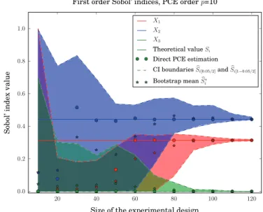
Fig. 4shows the evolution of the first order sensitivity indices (bSX1; bSX2; bSX3) versus the experimental design size for a Monte

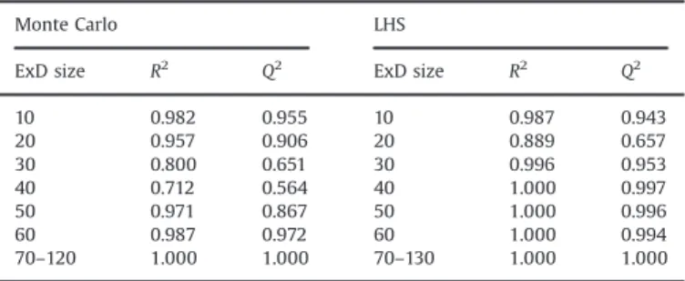
Carlo experimental design, whereas Fig. 5 presents the same results obtained with a LHS experimental design at each iteration. Legend Direct PCE estimation stands for sensitivity indices com-puted by PCE built on all the design of experiments. Finally, the values of R2 _{and Q}2 _{(see Section 2.3) versus the size of the}

experimental designs are also given inTable 3.

A similar study was carried out on total sensitivity indices and led to the same conclusions. First, we can observe that the meta-models, built on the whole experimental design, are generally more accurate with less points when a LHS experimental design is used, as shown by R2 _{and Q}2_{. It should also be noted that, for}

Fig. 2. Evolution of bSX1½0:05=2+vs. number of bootstrap samples B and size of the

experimental design N.

Fig. 3. Evolution of bSX1½1 ) 0:05=2+vs. number of bootstrap samples B and size of the

experimental design N.

Fig. 4. Evolution of first order sensitivity indices—Monte Carlo experimental design.

N 4 30, R2_{and Q}2 _{are quite different (especially for Monte Carlo}

design of experiment) which reveals the interest of the compar-ison between several indicators. Nevertheless, both design strate-gies lead to similar confidence interval convergence in a very close number of iterations. Finally, this numerical example does not allow to conclude on the interest of using LHS in our context.

4.1.4. Polynomial basis degree

We recall (seeSection 2.1) that the polynomial chaos expansion is based on a projection of the stochastic response onto a family of polynomials contained in a full candidate basis B, made of all suitable polynomials up to a degree p. This section is devoted to the choice of this degree p. In the previous examples, a large value of p was chosen because:

1. It is known that degree 7 is necessary to properly approximate the Ishigami function (see[26]).

2. The function has only 3 input parameters. So the time spent by the LAR algorithm remains reasonable.

Considering these two points, it is clear that, in an industrial case with many variables (greater than 10 for example), the size of the candidate basis B can make the LAR algorithm time consum-ing. Moreover choosing the degree a priori needs an expert judgment and, if it may be realistic in most of the cases, it could be sometimes difficult to evaluate the degree of the stochastic response. In order to tackle this problem, two different approaches are proposed and tested here.

1. If it is possible to have an accurate estimate of degree p (it is called pest) that is necessary to well approximate the response,

and if the number of variables is not too important, one can choose p ¼ p_estþ

δ

p where

δ

p is equal to 1, 2 or 3.

2. If the number of input parameters is important, we propose to choose p ¼ p_est, even if this value is hazardous. Then, the degree is increased following this empirical rule: if, after a few iterations (in practice four iterations appears as a good guess), the maximal confidence interval size is not divided by two, degree p of the candidate basis B is increased by one. As previously, these two strategies are illustrated on Ishigami function. For strategy ♯1, p is chosen equal to 10 and, for strategy ♯2, pestis chosen equal to 5 and 3.Fig. 6gives the results obtained

by the first strategy for which R2 _{and Q}2 _{values obtained with}

direct PCE construction are given byTable 3(Monte Carlo column).

Figs. 7and8correspond to the second one for p_est¼ 5 and p_est¼ 3 respectively and R2 _{and Q}2 _{values obtained with direct PCE}

construction are given byTable 4. In both cases, the experimental design is built by Monte Carlo sampling, confidence intervals are Table 3

Direct PCE estimation, R2_{and Q}2_{values—first order sensitivity indices, Monte Carlo} experimental design and LHS experimental design.

Monte Carlo LHS

ExD size R2 _Q2 _{ExD size R}2 _Q2

10 0.982 0.955 10 0.987 0.943 20 0.957 0.906 20 0.889 0.657 30 0.800 0.651 30 0.996 0.953 40 0.712 0.564 40 1.000 0.997 50 0.971 0.867 50 1.000 0.996 60 0.987 0.972 60 1.000 0.994 70–120 1.000 1.000 70–130 1.000 1.000

Fig. 6. Evolution of total sensitivity indices—first strategy—p¼10.

Fig. 7. Evolution of total sensitivity indices—second strategy—initial value of pest¼ 5—p increases by 1 at each vertical line.

Fig. 8. Evolution of total sensitivity indices—second strategy—initial value of pest¼ 3—p increases by 1 at each vertical line.

obtained by the percentile method with B¼700 and we look for the total sensitivity indices.

The comparison between the results of these two strategies allows us to show that, even if the expert judgment is bad (as in the second strategy), an increase of the degree based on the size of the confidence interval leads to convergence. Nevertheless, if pestis

far from the final value of p, the convergence becomes longer as illustrated by the case p_est¼ 3.

In conclusion, this section shows the importance of comple-mentarity between a correct degree p for the candidate basis B and enough points in the design of experiments. It also shows the capability of the method to converge even if the degree pest is

chosen far from what would be needed.

4.1.5. Type of confidence interval

Section 3.1 introduced three different bootstrap confidence intervals. We recall that the standard interval is based on an asymptotic approximation of the bootstrap distribution by a normal one. Despite the fact that [12] shows the asymptotic normality of Sobol' index estimator computed by Monte Carlo or by a convergent meta-model, the standard interval is not studied here because the hypothesis of normality of the bootstrap dis-tribution is never verified in practice (rejection of the assumption by the Kolmogorov normality test). In fact, as we proposed an adaptive design of experiment, at first iterations this asymptotic results are not yet verified and this type of CI is not adapted.

So this section discusses the difference between percentile bootstrap and the bias corrected and accelerated bootstrap (BCa).

First of all, some remarks have to be done on correction terms in the BCa method. These terms are numerically instable for small

size of design of experiments (first iterations of the proposed methodology). For example the acceleration terms a (see Eq.(7)) needs the calculation of statistics bSi ) j(evaluation of the sensitivity indices removing the jth sample point from the experimental design) and for small design of experiments, it happens that the best PCE is a constant. Then the sensitivity indices cannot be calculated and bSi ) j has no sense. The results for small design of experiments are not relevant and must be canceled from the conclusion. The last remark concerns the computational cost of the BCa. The calculation of the acceleration term is not negligible

because of the terms bSi ) j.

In order to compare the two types of confidence intervals, the example presented inFig. 8is considered. Total sensitivity indices are computed by a sparse PCE, the first degree p is chosen equal to 3, the experimental design is built by Monte Carlo sampling and the number of bootstrap samples is B¼700.Fig. 9presents results obtained with BCamethod. As previously, the R2and Q2values of

the PCE built on the experimental design at each iteration are provided inTable 5. It should be noted that these values are quite similar with the ones inTable 4as the same Monte Carlo sampling is used. Only the evolution of the degree p is different.

This figure clearly illustrates the stability problem of the BCa

method for small design of experiments. Then, compared toFig. 8

(same condition but CI constructed by percentile method), con-vergence is reached with a smaller design of experiments (150 points instead of 180) and final confidence intervals are centered on the theoretical values.

Finally, percentile and BCa methods give almost the same

results at the last iteration but BCaconverges faster and it is more

accurate in this example. Nevertheless, considering the instability problems for small design of experiments and the computational cost of this method, we will use the percentile method in the following example and compare with the BCamethod only in the

industrial application. Table 4

Direct PCE estimation, R2_{and Q}2 _{values—total sensitivity indices—p} est¼ 5 and pest¼ 3.

pest¼ 5 pest¼ 3

ExD size p R2 _Q2 _{ExD size p R}2 _Q2

10 5 0.480 0.171 10 3 0.480 0.171 20 5 0.714 0.543 20 3 0.000 ) 0.108 30 5 0.929 0.794 30 3 0.373 0.195 40 5 0.797 0.692 40 3 0.561 0.309 50 6 0.973 0.934 50 4 0.820 0.699 60 6 0.988 0.974 60 4 0.863 0.784 70 6 0.988 0.976 70 4 0.812 0.760 80 6 0.992 0.983 80 4 0.810 0.764 90 6 0.991 0.985 90 4 0.991 0.985 100 6 0.991 0.986 100 4 0.894 0.854 110 6 0.991 0.985 110 4 0.865 0.839 120 6 0.996 0.994 120 4 0.861 0.837 130 7 0.996 0.993 130 5 0.990 0.984 – – – – 140 5 0.989 0.984 – – – – 150 5 0.985 0.981 – – – – 160 5 0.985 0.981 – – – – 170 6 0.989 0.984

– – – – 180 6 0.989 0.985 Fig. 9. Evolution of total sensitivity indices—initial value of pest¼ 3—p increases by 1 at each vertical line—BCamethod.

Table 5

Direct PCE estimation, R2 _{and Q}2 _{values—total sensitivity indices—p} est¼ 3, BCa method. ExD size p R2 _Q2 10 3 0.480 0.171 20 3 0.000 ) 0.108 30 3 0.373 0.195 40 3 0.561 0.309 50 4 0.820 0.699 60 4 0.863 0.784 70 4 0.812 0.760 80 4 0.810 0.764 90 5 0.909 0.871 100 5 0.894 0.854 110 5 0.865 0.839 120 5 0.861 0.837 130 6 0.990 0.984 140 6 0.989 0.984 150 6 0.985 0.981

4.1.6. Convergence criterion

As defined inSection 3.2, convergence is reached when all the CIs sizes are less than x percent of the maximum bootstrap mean of the sensitivity indices. This part deals with the choice of parameter x. As an example, all previous figures were obtained with x ¼ 10%.

The choice of value x must be made according to the goal of the sensitivity analysis. If it only aims at ranking variables with a poor accuracy, a large value of x can be chosen (like 20 or 30). Conversely, if the sensitivity study has to be accurate (in order to work on variance reduction of some variables for example), value of x must be small (like 5 or 10).

Anyway, convergence is also depending on the maximum bootstrap mean of the sensitivity indices. It is impossible to know this value a priori but, as the sum of all first order sensitivity indices is one if there is no interaction, orders of magnitude given above will lead to correct results in almost every case. Problems will occur when the model has many variables of equal sensitivity indices or when the variables have their major effects in interac-tion. Then, a solution consists in following the convergence graph at each iteration and in deciding manually when to stop.

4.1.7. Conclusion

The previous numerical experiments on Ishigami function help us to draw some general conclusions on the methodology. First,

Section 4.1.2justifies the arbitrary choice B¼700, as it shows that, when the experimental design size increases, CIs boundaries become less sensitive to the value of B. Then, even if LHS leads to a better Q2_{, numerical tests using LHS to build and increase the}

design of experiments are not enough discriminatory (in terms of CIs size) to conclude about the efficiency of such method in our study. The choice of the basis degree p is, in an industrial context, linked to previous knowledges in the area. Anyway,Section 4.1.4

presents a simple way to increase this degree and find the correct one within a few iterations. Finally,Table 6gives some numerical comparison between the theoretical values and the results of the proposed algorithm. It allows one to be confident in the capability of the method. These results are obtained at last iteration of the algorithm with the following parameters: B¼700, p¼10, design of experiments built and increased by Monte Carlo sampling, con-vergence criterion fixed to 10%.

Considering all points discussed in this section, the methodol-ogy is now applied to the g-Sobol' function[21]with 8 parameters then to an industrial case.

4.2. Application to g-Sobol' function This function reads

Y ¼ ∏8 i ¼ 1

j4Xi) 2j þ ai 1 þ ai

;

where every Xi has a uniform distribution between 0 and 1.

Parameters ðaiÞ1 r i r 8 take their values in f0; 1; 4; 5; 9; 99; 99; 99g. Theoretical sensitivity indices are given inTable 7.

Our methodology is applied in order to determine the first order sensitivity indices. Parameters of the method, discussed in

Section 4, are set up as follows:

-

Number of bootstrap samples: B¼700.

-

Experimental design built by Monte Carlo sampling.

-

Degree of the polynomial basis B: p¼5.

-

_{Type of confidence interval: percentile}

-

Convergence criterion: maxðIC sizesÞ o0:1maxðE½bS_i+Þ.

Table 6

Ishigami function—comparison between theoretical and numerical sensitivity indices. S bS½α=2+ bS n b S½1 ) α=2+ ST bST½α=2+ bS n T bST½1 ) α=2+ X1 0.3138 0.3099 0.3143 0.3189 0.5574 0.5432 0.5561 0.5602 X2 0.4424 0.4396 0.4435 0.4565 0.4424 0.4400 0.4441 0.4572 X3 0.0000 0.0000 0.0000 0.0001 0.2436 0.2319 0.2421 0.2451 Table 7

g-Sobol function—first order and total sensitivity indices.

Variable Si STi X1 0.7165 0.7875 X2 0.1791 0.2423 X3 0.0237 0.0343 X4 0.0072 0.0105 X5;6;7;8 0.0001 0.0001

Fig. 10. Evolution of first order sensitivity indices—p¼5.

Table 8

Direct PCE estimation, R2 _{and Q}2 _{values—total} sensitivity indices—pest¼ 5.

ExD size R2 _Q2 40 0.843 0.788 70 0.940 0.919 100 0.986 0.977 130 0.991 0.981 160 0.978 0.971 190 0.985 0.978 Table 9

g-Sobol function—comparison between theoretical and numerical first order sensitivity indices.

Variable Si Lower CI boundary bSni Upper CI boundary

X1 0.7165 0.7000 0.7496 0.7919 X2 0.1791 0.1162 0.1504 0.1794 X3 0.0237 0.0069 0.0172 0.0301 X4 0.0072 0.0000 0.0038 0.0095 X5;6;7;8 0.0001 0.0000 0.0000 ½0:0001–0:0009+

Fig. 10shows the evolution of confidence intervals versus the number of iterations. As previously, R2_{and Q}2_{values are also given}

by Table 8. Table 9 gives a numerical comparison between theoretical values and estimations of the first order sensitivity indices obtained at last iteration.

This case shows that, when some variables have a major impact, it is not necessary to have a perfect approximation of the function to obtain accurate results on sensitivity indices. For example, the accuracy, related to results given in Table 9, is enough to select, rank variables and even to have correct relative importance information. Let us also remark that R2¼ 0:985 and Q2¼ 0:978 at the end of iterations. So an adaptive method, guided by values of R2

and Q2_{(targeting R}2_{40:99 or Q}2_{40:99 for example), would lead} in this case to a kind of over quality in the meta-model.

5. An industrial application: TARANIS 5.1. Context of the study

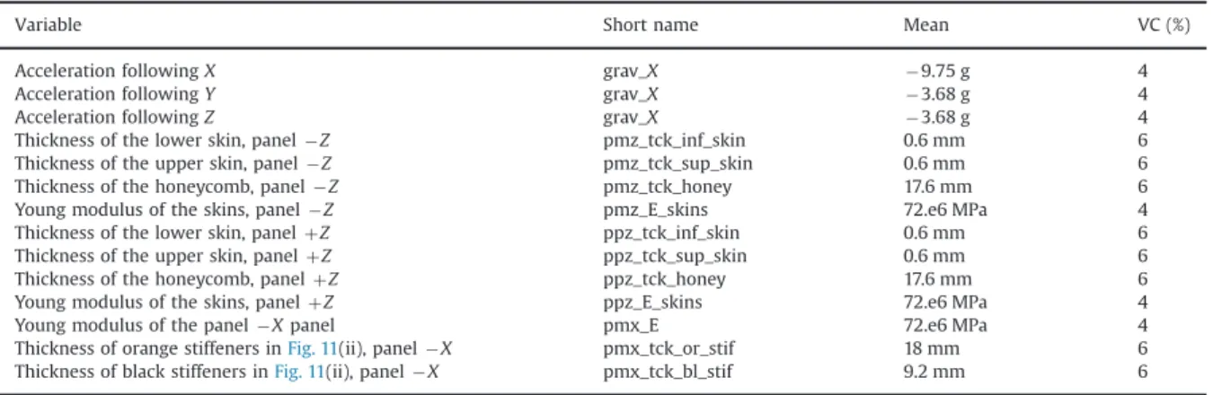
This example takes place in a reliability analysis of a satellite structure called TARANIS developed by CNES (Centre National d'Etudes Spatiales).Fig. 11shows the finite element model used for calculations (about 380,000 degrees of freedom). The aim of this work was to study the reliability under static load of the satellite using second order surface response (see[19]). Several methods were used to select the most relevant variables for every response and it appeared that 14 variables were sufficient.

More precisely, we focus here on one particular quantity of interest which is the maximum Von Mises stress in a particular panel under the following loading case: 9.75 g following X, ) 3.68 g following Y and 3.68 g following Z where g ¼ 9:81 m s) 2 is the gravity intensity.

The selected 14 variables are described in Table 10. All prob-ability densities are supposed to be Gaussian, means and variation coefficients (VCs) being given inTable 10. For this study, we aim at estimating the total sensitivity indices of every variable.

Following [19], a global sensitivity analysis was carried out using the calculation of sensitivity indices by Monte Carlo method on the surface response. This one was built using an experimental design of 186 points. Then, 2,000,000 Monte Carlo simulations of the surface response were necessary to obtain the sensitivity indices. Results are presented inTable 11, Column R-S. It can be noticed that the sum of all indices is close to one, which means there is almost no interaction between variables.

5.2. Results obtained with bootstrap re-sampling and polynomial chaos expansion

The algorithm presented inSection 3.2is applied to the study of the total sensitivity indices of the 14 variables introduced previously. The parameters of the method are

-

Number of bootstrap samples: B¼700.

-

Experimental design built by Monte Carlo sampling.

Fig. 11. (i) Finite element model of Taranis structure, (ii) Minus X panel.

Table 10

Gaussian variables for the TARANIS model.

Variable Short name Mean VC (%)

Acceleration following X grav_X ) 9.75 g 4

Acceleration following Y grav_X ) 3.68 g 4

Acceleration following Z grav_X ) 3.68 g 4

Thickness of the lower skin, panel ) Z pmz_tck_inf_skin 0.6 mm 6 Thickness of the upper skin, panel ) Z pmz_tck_sup_skin 0.6 mm 6 Thickness of the honeycomb, panel ) Z pmz_tck_honey 17.6 mm 6 Young modulus of the skins, panel ) Z pmz_E_skins 72.e6 MPa 4 Thickness of the lower skin, panel þ Z ppz_tck_inf_skin 0.6 mm 6 Thickness of the upper skin, panel þ Z ppz_tck_sup_skin 0.6 mm 6 Thickness of the honeycomb, panel þ Z ppz_tck_honey 17.6 mm 6 Young modulus of the skins, panel þ Z ppz_E_skins 72.e6 MPa 4

Young modulus of the panel ) X panel pmx_E 72.e6 MPa 4

Thickness of orange stiffeners inFig. 11(ii), panel ) X pmx_tck_or_stif 18 mm 6 Thickness of black stiffeners inFig. 11(ii), panel ) X pmx_tck_bl_stif 9.2 mm 6

-

Convergence criterion: maxðIC sizesÞo 0:1maxðE½bSi+Þ.

-

_{Type of confidence interval: percentile.}

-

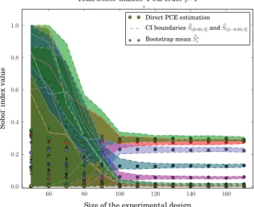
Degree p of the polynomial basis B: three choices are tested. First, p¼ 2 and it may increase; second, p¼ 3 and it cannot increase; finally, p¼4 and it cannot increase.

Fig. 12gives the evolution of the sensitivity indices when p¼2, the vertical lines meaning an increase of one in the maximal

degree of the candidate basis.Figs. 13and14depict this evolution for p¼3 and p¼4 respectively.

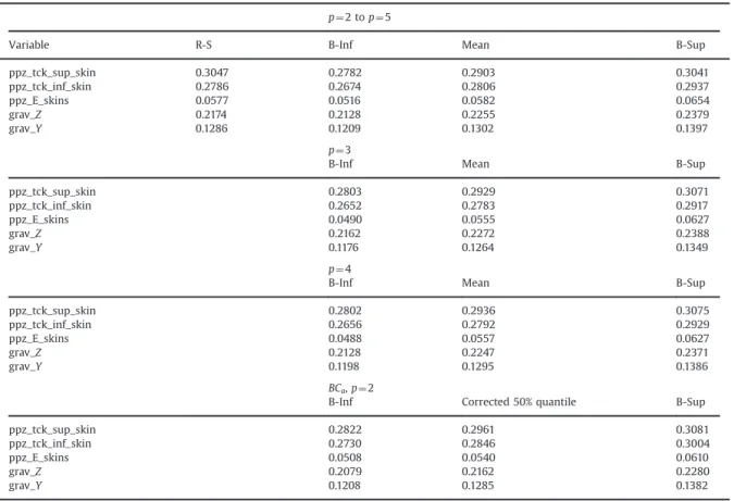
These figures exhibit an interesting phenomenon. If the degree p of the full candidate basis B is high (Fig. 14), at first iterations, 100 points are necessary to reach correct CIs sizes. This shows that, if the candidate basis size is too large, the selection algorithm is disturbed and this leads to large CIs. Anyway, as a severe convergence criterion is chosen (x ¼10), all choices converge between 160 (p¼3) and 190 (p¼2–5). But if the convergence Table 11

Comparison between surface response method and bootstrap re-sampling on sensitivity indices computed by PCE.

p¼ 2 to p¼ 5

Variable R-S B-Inf Mean B-Sup

ppz_tck_sup_skin 0.3047 0.2782 0.2903 0.3041 ppz_tck_inf_skin 0.2786 0.2674 0.2806 0.2937 ppz_E_skins 0.0577 0.0516 0.0582 0.0654 grav_Z 0.2174 0.2128 0.2255 0.2379 grav_Y 0.1286 0.1209 0.1302 0.1397 p¼ 3

B-Inf Mean B-Sup

ppz_tck_sup_skin 0.2803 0.2929 0.3071 ppz_tck_inf_skin 0.2652 0.2783 0.2917 ppz_E_skins 0.0490 0.0555 0.0627 grav_Z 0.2162 0.2272 0.2388 grav_Y 0.1176 0.1264 0.1349 p¼ 4

B-Inf Mean B-Sup

ppz_tck_sup_skin 0.2802 0.2936 0.3075 ppz_tck_inf_skin 0.2656 0.2792 0.2929 ppz_E_skins 0.0488 0.0557 0.0627 grav_Z 0.2128 0.2247 0.2371 grav_Y 0.1198 0.1295 0.1386 BCa, p¼2

B-Inf Corrected 50% quantile B-Sup

ppz_tck_sup_skin 0.2822 0.2961 0.3081

ppz_tck_inf_skin 0.2730 0.2846 0.3004

ppz_E_skins 0.0508 0.0540 0.0610

grav_Z 0.2079 0.2162 0.2280

grav_Y 0.1208 0.1285 0.1382

criterion is relaxed at x ¼20, the first choice (p¼2–5) converges faster than the two others.

Finally, the BCa method for the construction of sensitivity

indices is also tested, with p¼2, all other parameters remaining the same.Fig. 15presents this case.

The comparison betweenFig. 15(using BCa) andFig. 12(using

percentiles) reveals almost no difference between the two con-struction methods for the confidence intervals. This seems to show that for smooth responses, the BCa method gives no advantage

compared to the percentile one.Table 11summarizes all results. A comparison with the results obtained by the response surface method allows one to be confident in the capability of the method for solving industrial problems, as both methods lead to the same conclusion. Moreover confidence intervals, that are built by boot-strap re-sampling, also contain results given by the response surface method, which show the relevance of these intervals.

6. Conclusion

The methodology proposed in this paper aims at combining advantages of PCE with bootstrap re-sampling for the determination

of sensitivity indices of industrial models with a given degree of confidence. First of all, an efficient computation of sensitivity indices is obtained thanks to the PCE construction presented in[3]. Then, in order to evaluate confidence intervals for these estimated sensitivity indices, bootstrap re-sampling is applied to the design of experi-ments that is used to build the PCE. New PCE are constructed on each bootstrap sample, which leads to a collection of sensitivity indices and, finally, to empirical confidence intervals for every sensitivity index. Moreover, the iterative procedure introduced inSection 3.2

guides the construction of an adaptive experimental design to reach an accuracy objective, expressed on the sensitivity indices and not on the quality of the meta-model. Finally, this leads to an optimized design of experiments for the determination of sensitivity indices. Comparisons with classical meta-model error estimators show that, in some cases, confidence intervals on sensitivity indices are accurate enough whereas global error estimators on meta-model are bad (for example, see values of Q2_{and R}2_{in the g-Sobol function compared to}

the size of confidence intervals). This reveals the interest of a sensitivity-indices-oriented methodology.

Nevertheless, this algorithm requires to set up five parameters. Their influence is discussed alongSection 4and allows to draw some conclusions:

-

_{The number of bootstrap re-sampling B has to be sufficient to}

guarantee the convergence of the empirical confidence inter-vals. A convergence analysis as a function of B was carried out and the choice B¼700 appears to be a good one. This analysis also indicates that it is a conservative way to choose B.

-

To create and increase the design of experiments, we use Monte Carlo sampling and LHS. It seems that LHS do not improve efficiency of the method.

-

The degree p of the full candidate polynomial basis B has to be chosen in priority according to previous knowledge. If it is not possible, it seems that an acceptable choice for most elastic stress analysis problems is p¼3. Anyway, a method to increase this degree, linked to the size of confidence intervals, is tested and always leads to correct results in the presented applica-tions. Note that, if it seems comfortable to choose an a priori high degree, it may perturb the PCE construction and slow down the convergence, as shown by the industrial application.

-

_{Confidence intervals are mainly constructed using the}

percen-tile method. In the case of the Ishigami function the BCa

method converges faster but this conclusion is not confirmed by the industrial example. To conclude, in our application area, it seems that the BCa procedure is not recommended as its

numerical cost is important (compared to percentile method) and improvement in the convergence is not guaranteed.

-

A convergence criterion, based on the size of the confidence intervals, has to be chosen according to the aim of sensitivity analysis. As seen inSection 4, one must keep in mind that a low convergence criterion can lead to an important number of iterations. A safer way is then to start from a high value, to observe results and then to restart the algorithm from this new starting point with a lower convergence criterion if previous results are not accurate enough.

Finally, let us discuss the numerical cost of the methodology. The number of evaluations of the numerical model used to build the PCE (i.e. the size of the final design of experiments) is supposed to be almost optimized for the aim of the PCE. Nevertheless, using a LHS design of experiments generally decreases the number of points needed to build PCE with a given accuracy on a global error criterion. The fact that our methodology is not sensitive to this LHS property seems to be due to bootstrap re-sampling. The computa-tional time devoted to bootstrap re-sampling, is a function of the number B of samples and the complexity in the construction of the Fig. 14. Evolution of total sensitivity indices—p¼4.

PCE (number of input variables, size of the candidate polynomial bases), as B new PCE are built. In comparison with the solutions used in[20]and[13], where the polynomial basis does not change and only coefficients of the expansion are recalculated (least square minimization), our methodology is more expensive (B basis selec-tions instead of 1) but it allows to take into account variaselec-tions in the polynomial selection process.

Acknowledgments

This work was partially supported by Centre National d'Etudes Spatiales and Thales Alenia Space. The authors would like to thank Nicolas Roussouly for fruitful discussions and reviewers for their relevant comments.

References

[1]Blatman G. Adaptive sparse polynomial chaos expansions for uncertainty propagation and sensitivity analysis. PhD thesis, Université Blaise Pascal, Clermont-Ferrand, 2009.

[2]Blatman G, Sudret B. An adaptive algorithm to build up sparse polynomial chaos expansions for stochastic finite element analysis. Probabilistic Engineer-ing Mechanics 2010;25:183–97.

[3]Blatman G, Sudret B. Adaptive sparse polynomial chaos expansion based on least angle regression. Journal of Computational Physics 2010;230:2345–67. [4]Blatman G, Sudret B. Efficient computation of global sensitivity indices using

sparse polynomial chaos expansions. Reliability Engineering & System Safety 2010;95(11):1216–29.

[5]Castaings W, Borgonovo E, Morris MD, Tarantola S. Sampling strategies in density-based sensitivity analysis. Environmental Modelling & Software 2013;38:13–26.

[6]Cornillon PA, Matzner-Lober E. Régression théorie et applications. Springer; 2007.

[7]DiCiccio TJ, Efron B. Bootstrap confidence intervals. Statistical Science 1996;11 (3):189–228.

[8]Efron B. Better bootstrap confidence intervals. Journal of the American Statistical Association 1987;82(397):171–85.

[9]Efron B, Hastie T, Johnstone I, Tibshirani R. Least angle regression. Annals of Statistics 2004;32:407–99.

[10]Efron B, Tibshirani RJ. An introduction to the bootstrap. New York: Chapman & Hall; 1993.

[11] Gayton N, Bourinet JM, Lemaire M. CQ2RS: a new statistical approach to the response surface method for reliability analysis. Structural Safety 2003;25 (1):99–121.

[12]Janon A, Klein T, Lagnoux A, Nodet M, Prieur C. Asymptotic normality and efficiency of two Sobol’ index estimators. Technical report, INRIA, 2012.

[13]Janon A, Nodet M, Prieur C. Confidence intervals for sensitivity indices using reduced-basis metamodels. Technical report, INRIA, 2010.

[14]Lemaire M. Fiabilité des structures –Couplage mécano-fiabiliste statique. Hermès; 2005.

[15]Mallows CL. Some comments on Cp. Technometrics 2000;42(1):87–94. [16]Notin A, Gayton N, Dulong JL, Lemaire M, Villon P. RPCM: a strategy to perform

reliability analysis using polynomial chaos and resampling—application to fatigue design. European Journal of Computational Mechanics 2010;19 (8):795–830.

[17] Plischke E, Borgonovo E, Smith CL. Global sensitivity measures from given data. European Journal of Operational Research 2013;226:536–50.

[18]Rahman S. Global sensitivity analysis by polynomial dimensional decomposi-tion. Reliability Engineering & System Safety 2011;96(7):825–37.

[19]Roussouly N. Approche probabiliste pour la justification par analyse des structures spatiales. PhD thesis, Université de Toulouse, Toulouse, 2011.

[20] Roussouly N, Petitjean F, Salaün M. A new adaptive response surface method for reliability analysis. Probabilistic Engineering Mechanics 2013;32:103–15. [21]Saltelli A, Chan K, Scott EM, editors. Sensitivity analysis. John Wiley & Sons;

2000.

[22] Sobol' IM. Sensitivity estimates for nonlinear mathematical models. Mathe-matical Modeling 1993;1:407–14.

[23] Sobol' IM. Global sensitivity indices for nonlinear mathematical models and their Monte Carlo estimates. Mathematical Models and Computer Simulations 2001;255:271–80.

[24] Soize C, Ghanem R. Physical systems with random uncertainties: chaos representations with arbitrary probability measure. SIAM Journal on Scientific Computing 2004;26(2):395–410.

[25] Storlie CB, Swiler LP, Helton JC, Sallaberry CJ. Implementation and evaluation of nonparametric regression procedures for sensitivity analysis of computa-tionally demanding models. Reliability Engineering & System Safety 2009;94:1735–63.

[26] Sudret B. Global sensitivity analysis using polynomial chaos expansions. Reliability Engineering & System Safety 2008;93(7):964–79.

[27]Xiu D, Karniadakis GE. The Wiener–Askey polynomial chaos for stochastic differential equations. SIAM Journal on Scientific Computing 2002;24 (2):619–44.