An efficient and flexible software tool for genome-wide association interaction studies

(1)

University of Liège

Faculty of Applied Sciences

Department of Electrical Engineering and Computer Science

Montefiore Institute

An Efficient and Flexible

Software Tool

for

Genome-Wide Association

Interaction Studies

-Academic year

2015-2016

PhD thesis by

Van Lishout François

Promotor

(2)

Jury members

Boigelot Bernard (president) Professor, University of Liège (Montefiore Institute)

Van Steen Kristel (promotor) Professor, University of Liège (GIGA-R)

Wehenkel Louis Professor, University of Liège (Montefiore Institute)

Farnir Frédéric Professor, University of Liège (Faculty of Veterinary Medicine)

König Inke Professor, University of Lübeck (Med. Biometrie & Stat. Inst.)

Van der Spek Peter Professor, Erasmus MC Rotterdam (Bioinformatics Department)

Liège, 2016

Thesis submitted in fulfilment of the requirements for the degree of Doctor in Electrical Engineering and Computer Science

(3)

Acknowledgements

First of all, I would like to express my deepest gratitude to my promotor, professor Kristel Van Steen. She gave me the chance to work in a good multi-cultural environ-ment on a very interesting subject, both from a theoretical and a practical point of view. With her, I learned many important aspects of conducting a research project successfully to its end. In the earlier days of this thesis, few people believed that the MB-MDR methodology could one day allow genome-wide association interaction stud-ies. However, Kristel Van Steen did and gave me the opportunity to help her proving it. Despite the fact that this task seemed almost impossible to me, I trusted her and worked over the years in speeding up the methodology, to finally prove her right.

Second, I would like to thank Louis Wehenkel. He is truly the one who discovered my research skills, at a time when I was still master student and did not see them myself. After having worked as a software developer in industry for some years, my way came across his again and he offered me a position at the GIGA. Then, he introduced me to Kristel Van Steen and she made this PhD project possible. I would also like to thank Louis Wehenkel for the long and instructive discussions that we had over the years, about and around my PhD thesis. Finally, let me mention that working as a teaching assistant for him was always a real pleasure to me.

I am very grateful to the staff of the Electrical Engineering and Computer Science Department of the University of Liège, for all the help given. A special thanks to my col-leagues Jestinah Mahachie John, Elena Gusareva, Kirill Bessonov, Francesco Gadaleta and Tom Cattaert who contributed heavily to my work and published with me. In ad-dition, I would also like to mention Bärbel Maus, Ramouna Fouladi, Benjamin Dizier, Raphael Liégeois, Alejandro Marcos Alvarez, Cyril Soldani, Pierre Geurts, Damien Ernst, Guillaume Drion, Samuel Hiard, Julien Becker and many more with whom I had very interesting research talks that helped me to conceptualize my ideas.

My gratitude goes to my jury members, for taking the time to read and evaluate my thesis. I would also like to thank all the international collaborators that I interacted with in the course of my PhD: Jason Moore, Damian Gola, Malu Calle, Viktor Urea, Duan Quingling, Kelan Tantishira, Isabelle Cleynen, Céline Vens, Lars Wienbrandt and many more.

My most affectionate thanks go to my family. My mother Myriam Kremers, who was always there to listen to me in the moments of doubts. In the memory of my father Pierre Van Lishout, who taught me how to give my best in everything I do. My girl Célia Van Lishout, who is truly my sunshine. I went to some difficult moments in the last two years and she was really the one who gave me the energy to go through them. François Van Lishout

(4)

Abstract

Humans are made up of approximately 3.2 billion base pairs, out of which about 62 million can vary from one individual to another. These particular base pairs are called single nucleotide polymorphisms (SNPs). It is well known that some particular combination of SNP values increase dramatically the risk of contracting certain type of disease, like Crohn’s disease, Alzheimer, diabetes and cancer, just to name a few. However, there are still a lot of new discoveries to make and specialized software is required for this task.

It has been shown that individual SNPs cannot account for much of the heritabil-ity on their own. Therefore, this PhD thesis is dedicated to interaction studies, the purpose of which is to identify pairs of SNPs and/or environmental factors that might regulate the susceptibility to the disease under investigation. Model-Based Multifac-tor Dimensionality Reduction (MB-MDR) is a powerful and flexible methodology to perform interaction analysis, while minimizing the amount of false discoveries.

Before this thesis, the only available implementation was an R-package taking days to analyze a dataset composed of just hundred of SNPs. However, a typical dataset contains hundreds of thousands or millions of SNPs, even after data cleaning and quality control. The aim of this thesis is to write a software able to analyze such datasets within a few days with the MB-MDR methodology. In other words, the goal is to get 108 _{times faster than the R-package, while still remaining powerful, flexible}

and keeping the amount of false discoveries low.

Several contributions were needed to reach this goal and are presented in this thesis. First, a new software was written from scratch in C++, in order to be able to optimize every single computation, instead of relying on too generic functions as was the case for the R-package. Second, the methodology itself was improved, irrespective of the programming language. Indeed, MB-MDR is based on the maxT algorithm (introduced by Westfall&Young in 1993) to assess significance of the results and it can be customized

for interaction analysis. A first major contribution of this PhD work, called Van

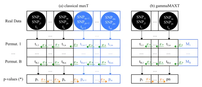
Lishout’s implementation of maxT, was introduced in 2011. The parallel version of this algorithm enables to analyze a dataset composed of hundred thousands of SNPs within a few days. The most important contribution of this thesis, called the gammaMAXT algorithm, was introduced in 2014. The parallel version enables to analyze a dataset composed of one million SNPs within one day.

In this thesis, we also propose a new viewpoint to handle population stratification and correct for covariates. Many simulated and real-life data analysis are provided, to highlight the flexibility of the software and its ability to find interesting results from a biological point of view. The latest version, called mbmdr-4.4.1.out, can be downloaded freely at http://www.statgen.ulg.ac.be with the corresponding documentation.

(5)

Résumé

L’homme est composé d’approximativement 3,2 milliards de paires de bases, dont plus ou moins 62 millions peuvent varier d’un individu à l’autre. Ces paires de bases variant d’un individu à l’autre sont appelées des SNPs (polymorphisme d’un seul nucléotide). Il est un fait avéré que certaines combinaisons de valeurs de SNPs augmentent fortement les chances de contracter certaines maladies comme la maladie de Crohn, Alzheimer, le diabète et le cancer pour n’en citer que quelques unes. Par contre, il reste encore beaucoup de découvertes à faire et le développement de software spécialisé est nécessaire pour y parvenir.

Il a été montré qu’un SNP ne peut à lui seul apporter beaucoup d’information sur l’héritabilité d’une maladie. Par conséquent, ce doctorat est consacré aux études d’interactions, dont l’objet est d’identifier des paires de SNPs et/ou de facteurs en-vironnementaux pouvant réguler la susceptibilité à contracter la maladie étudiée. La méthodologie MB-MDR (Model-Based Multifactor Dimensionality Reduction) est une technique puissante et flexible permettant d’effectuer des études d’interactions, tout en minimisant le nombre de fausses découvertes.

Avant cette thèse de doctorat, la seule implémentation disponible de cette méthodolo-gie était un package écrit en R, prenant des jours pour analyser un des données con-tenant à peine quelques centaines de SNPs. Or, un jeu de données typique est à l’heure actuelle composé de centaines de milliers voir de millions de SNPs et ce même après avoir épuré les données et réalisé différents contrôles de qualité. L’objectif de ce doc-torat est d’écrire un logiciel capable d’analyser ce genre de données en quelques jours

à l’aide de la méthodologie MB-MDR. En d’autres mots, il s’agit de devenir 108 _fois

plus rapide que le package écrit en R, tout en restant au moins aussi puissant et rapide qu’avant et en maintenant un nombre minimum de fausses découvertes.

Plusieurs contributions furent nécessaires pour y arriver. Premièrement, un nou-veau logiciel a été développé en C++ en partant de zéro et ceci afin d’optimiser toutes les opérations effectuées plutôt que de se baser sur des fonctions trop génériques comme c’était le cas dans le package R. Deuxièmement, la méthodologie elle-même a dû être améliorée et ce indépendamment du choix du langage de programmation. En effet, MB-MDR est basé sur l’algorithme maxT (Westfall & Young 1993) pour estimer la pertinence des résultats et cet algorithme a du être customisé pour le cas partic-ulier des études d’interactions. Ainsi, la première contribution majeure de cette thèse, l’implémentation Van Lishout de maxT, a été proposée en 2011. La version parallèle permet d’analyser un jeu de données composé de cent mille SNPs en quelques jours. La contribution principale de ce doctorat est l’algorithme gammaMAXT, introduit en 2014. La version parallèle permet d’analyser un dataset composé d’un million de SNPs en un seul jour.

(6)

v

Cette thèse présente également un nouveau point de vue pour tenir compte de la stratification de la population et corriger les covariables. De nombreuses analyses de données (simulées ou réelles) sont également décrites dans ce manuscrit, pour mettre en évidence la flexibilité du software et sa capacité à découvrir des résultats intéressants d’un point de vue biologique. La version la plus récente du logiciel, mbmdr-4.4.1.out, peut être téléchargée gratuitement sur le site http://www.statgen.ulg.ac.be, avec la documentation correspondante.

(7)

List of Figures

1.1 Single Nucleotide Polymorphism . . . 2

2.1 Epistasis . . . 6

2.2 Input/output of mbmdr-4.4.1.out . . . 7

2.3 Case-control studies . . . 8

2.4 MDR methodology . . . 9

2.5 MB-MDR methodology: binary trait . . . 10

2.6 Binary MB-MDR statistic computing (no 1st order correction) . . . 11

2.7 MB-MDR methodology: continuous trait . . . 25

2.8 Continuous MB-MDR statistic computing (no 1st _{order correction) . . .} ₂₆

2.9 MB-MDR methodology: survival trait . . . 39

2.10 Survival MB-MDR statistic computing (no 1st _{order correction)} _{. . . .} ₄₁

2.11 Likelihood versus Wald versus score test . . . 51

2.12 Mutual Information . . . 53

3.1 Minimizing the work of the biologist . . . 56

3.2 Bonferroni correction . . . 58

3.3 Memory usage: classical Bonferroni vs mbmdr-4.4.1.out implementation 61 3.4 MaxT intuitive idea . . . 62

3.5 Classical maxT implementation . . . 64

3.6 Classical implementation of maxT versus Van Lishout’s one . . . 66

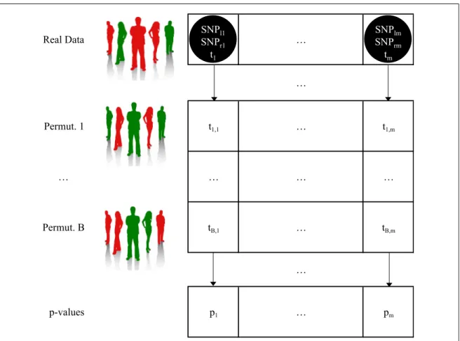
3.7 Parallel workflow of Van Lishout’s implementation of maxT . . . 71

3.8 Classical maxT versus gammaMAXT . . . 75

3.9 Theoretical versus predicted Mi values for dataset D1 . . . 79

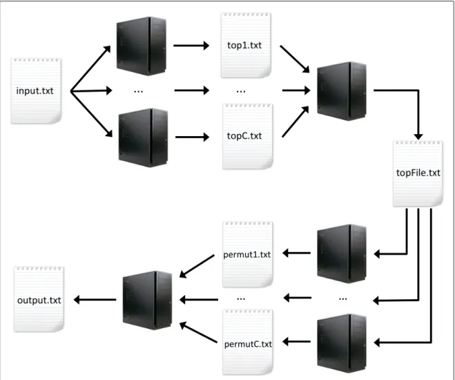
3.13 Parallel workflow of gammaMAXT algorithm . . . 85

3.14 Classical minP implementation . . . 91

3.15 Ge’s implementation of minP versus Van Lishout’s one . . . 94

4.1 Confounding factor definition . . . 100

4.2 Population stratification example . . . 101

4.3 STRAT1 algorithm (basic idea) . . . 104

4.4 STRAT1 algorithm (practical implementation) . . . 106

4.5 STRAT2 algorithm (basic idea) . . . 108

4.6 MB-MDR statistic computing with on-the-fly correction: binary trait . 122 4.7 SNP Finder hit for IBD . . . 135

4.8 Venn diagram of the results of Table 4.12 . . . 137

(10)

Résumé

(11)

List of Tables

1.1 Available features in some common association interaction studies software 3

3.1 Type I and type II errors in GWAIs . . . 57

3.2 Two-locus penetrance table used to create the simulated data . . . 70

3.3 Execution times of R package and mbmdr-2.6.2.out . . . 70

3.4 Execution times of the sequential and parallel versions of mbmdr-3.0.3.out 72

3.5 Number of test-statistics computed within the different steps of Van

Lishout’s implementation of MaxT on a dataset containing 103 subjects

and 106 _{SNPs. . . .} ₇₃

3.6 Two-locus penetrance table used to create the simulated datasets D1,

D2 and D3 . . . 78

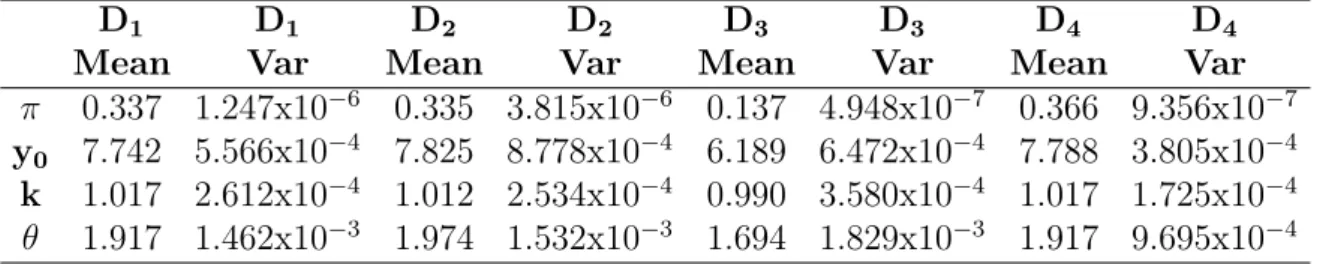
3.7 Mean and variance of the fitted parameters for datasets D1− D4 . . . . 83

3.8 Execution times of the sequential and parallel versions of mbmdr-4.2.2.out 86

3.9 Observed FWER of mbmdr-4.2.2.out . . . 88

3.10 Power comparison between the gammaMAXT and the MaxT algorithms 89

4.1 SNP pairs having a p-value < 0.05 on the discovery data with

gamma-MAXT . . . 111

4.2 SNP pairs having a p-value < 0.05 on the discovery and replication

data, using gammaMAXT on the discovery data and STRAT2 on the replication one. . . 112

data, using gammaMAXT on the replication data and STRAT2 on the discovery one. . . 113

4.4 SNP pairs having a p-value < 0.05 on the discovery data, using

gamma-MAXT with residuals-based correction of gender. . . 116 4.5 SNP pairs having a p-value < 0.05 on the discovery and replication data,

using each time gammaMAXT with residuals-based correction of gender. 117 4.6 SNP pairs having a p-value < 0.05 on the discovery and replication data,

using each time gammaMAXT with residuals-based correction of the top 10 PCs. . . 118

4.7 SNP pairs having a p-value < 0.05 on the discovery data, using

gamma-MAXT with on-the-fly correction of gender. . . 131 4.8 SNP pairs having a p-value < 0.05 on the discovery and replication data,

using each time gammaMAXT with on-the-fly correction of gender. . . 132

data, using each time gammaMAXT with on-the-fly correction of cluster membership. . . 133

4.10 Promising SNP pairs to investigate from a biological point of view. . . 134

(12)

Résumé

4.12 Amount of SNP pairs having a p-value < 0.05 on the discovery data, on the replication data and on both datasets, depending on the method used.137 5.1 SNP-SNP interactions having a multiple testing corrected p-value < 0.05 141

5.2 Location of the SNPs involved in a significant SNP-SNP interaction . . 141

5.3 Significant SNP-environment pairs found with LD pruning at 0.05 . . . 145

5.4 Significant SNP-environment pairs found with LD pruning at 0.2 . . . . 145

5.6 Significant SNP-environment pairs found with LD pruning at 0.75 . . . 145

5.8 Significant SNP-SNP-environment triplets found with LD pruning at 0.2 146

5.9 Percentage of times that the causal pair is found (200 individuals) . . . 148

5.10 Percentage of times that the causal pair is found (400 individuals) . . . 149 5.11 Percentage of times that the causal pair is found (800 individuals) . . . 149 5.12 Percentage of times that the causal pair is found (1600 individuals) . . 149 5.13 Percentage of datasets leading to at least one false-positive (200 subjects)150 5.14 Percentage of datasets leading to at least one false-positive (400 subjects)150 5.15 Percentage of datasets leading to at least one false-positive (800 subjects)150 5.16 Percentage of datasets leading to at least one false-positive (1600 subjects)150 5.17 Significant SNP-SNP pairs found for CAD, without covariate correction 154 5.18 Significant SNP-SNP pairs found for CAD, corrected for gender and age 154

(13)

List of Algorithms

Box 2.1. Binary MB-MDR statistic computing (no 1st order correction) . . . . 13

Box 2.2. Model fitting using IRLS . . . 16

Box 2.3. Binary MB-MDR statistic computing (with 1st _{order correction) . . .} ₁₈

Box 2.4. Binary main effect statistic computing . . . 20

Box 2.5. Binary three-order statistic computing (no 1st _{order correction) . . . .} ₂₁

Box 2.6. Continuous MB-MDR statistic computing (no 1st _{order correction) . .} ₂₈

Box 2.7. Model fitting for a continuous trait . . . 30

Box 2.8. Continuous MB-MDR statistic computing (with 1st _{order correction) .} ₃₃ Box 2.9. Continuous main effect statistic computing . . . 35

Box 2.10. Continuous 3D statistic computing (no 1st order correction) . . . 36

Box 2.11. Survival MB-MDR statistic computing (no 1st _{order correction)} _{. . .} ₄₂

Box 2.12. Survival MB-MDR statistic computing (with 1st _{order correction) . .} ₄₈

Box 3.1. mbmdr-4.4.1.out’s implementation of Bonferroni . . . 60

Box 3.2. Van Lishout’s implementation of maxT . . . 69

Box 3.3. Step 2(b) of gammaMAXT . . . 83

Box 3.4. Algorithm for sampling Mi when CDF is given by FZi(z) . . . 84

Box 3.5. Van Lishout’s implementation of minP . . . 96

Box 4.1. Fast Algorithm for Median Estimation . . . 105

Box 4.2. STRAT1 algorithm . . . 105

Box 4.3. STRAT2 algorithm . . . 109

Box 4.4. Survival MB-MDR statistic with on-the-fly correction . . . 120

Box 4.5. Binary MB-MDR statistic with on-the-fly correction . . . 126

(14)

Chapter 1 General introduction

Public health genomics proposes to use genomic information to improve public health. The aim is to perform an effective and responsible translation of genome-based knowl-edge into public health policy and health services. One aspect of it is to assess the impact of genes and their interaction with environmental factors on human health. This research field is very wide and includes association studies, health prediction and descriptive genomics. Two major aims of the former are reaching a better un-derstanding of the underlying mechanism behind diseases and identifying risk factors. The long-term ambition of predictive methods is to reach a personalized medicine, for which healthcare would be customized, i.e. based on molecular analysis and for in-stance clinical/familial history and lifestyle [106, 128, 37, 6, 71]. The main objective of descriptive genomics is molecular reclassification of subjects, using pattern recognition in a supervised or unsupervised way. This PhD thesis focuses on association studies.

Deoxyribonucleic acid (DNA) is the hereditary material of all known living organ-isms and many viruses. Most DNA molecules consist of two strands coiled around each other to form the famous double helix. The two DNA strands are composed of sim-pler units called nucleotides. Each nucleotide is composed of a chemical base - either adenine (A), thymine (T), cytosine (C), or guanine (G) - as well as a monosaccharide sugar called deoxyribose and a phosphate group. A critical feature of DNA is the abil-ity of the nucleotides to make specific pairs: adenine pairs with thymine and cytosine with guanine. A gene is a region (locus) of DNA that encodes a functional ribonucleic acid (RNA) or protein product. RNA is a polymeric molecule assembled as a chain of nucleotides, which is more often found in nature as a single-strand folded onto itself, rather than a paired double-strand as for DNA molecules. Mutations can occur within genes, leading to different variants of the gene in the population, known as alleles.

The Human Genome Project (1990-2003), allowed the release of the first human reference genome by determining the sequence of about 3.2 billion base pairs and identifying the approximately 22 thousand human genes [55, 69, 72]. It comes without saying that nucleotides not differing from one individual to another cannot regulate susceptibility to disease. The focus in this thesis is therefore on the approximately 62 million remaining ones [89], called single nucleotide polymorphisms (SNPs) and illustrated in Figure 1.1. Note that the methods presented in this work are generic. As a consequence, other forms of polymorphisms can also be handled (for instance human hemoglobin and blood groups) and other species than humans can be studied.

(15)

Chapter 1

Source: http://www.dnabaser.com/articles/SNP/SNP-single-nucleotide-polymorphism.html

Figure 1.1: A Single Nucleotide Polymorphism (SNP) is a DNA sequence variation in which a nucleotide in the genome differs between members of species. In this example, fragment 1 and 2 differ at a single base-pair location.

Genome-wide association studies (GWAs), using a dense map of SNPs, have become one of the standard approaches for unraveling the basis of complex genetic diseases [47]. However, significant genetic variants discovered in GWAS explain only a small proportion of the expected narrow-sense heritability, defined as the ratio of additive genetic variance to phenotypic variance [84, 29]. This is known as the missing her-itability problem, i.e. the fact that individual genes cannot account for much of the heritability of phenotypes [109, 70]. Focusing on the combined effect of all the genes in the background, rather than on the disease genes in the foreground, is a promising idea for estimating heritability [145]. This PhD thesis is dedicated to genome-wide association interaction studies (GWAIs), the purpose of which is to identify pairs of SNPs that might regulate the susceptibility to the disease under investigation. Further-more, we are particularly interested in detecting epistasis, occurring when the effect of one gene depends on the presence of one or more modifier genes. Epistatic inter-actions occur whenever one mutation alters the local environment of another residue (either by directly contacting it, or by inducing changes in the protein structure) [48]. Experimental studies in model organisms have demonstrated evidence of biological in-teractions among genes [78]. Furthermore, finding pairwise inin-teractions opens the door for constructing statistical epistasis networks, that allows a better understanding of the biochemical mechanisms of complex diseases, as was demonstrated in the context of bladder cancer [118]. As an extension, we are also interested in genome-wide envi-ronmental interaction studies (GWEIs), whose aim is to identify gene-envienvi-ronmental factors interactions (for environmental factors such as age, gender, etc) [3]. Nowadays, a lot of genetical and/or environmental interactions impacting susceptibility to diseases still needs to be identified and dedicated software is needed for this task. The aim of this PhD is to develop an efficient and flexible software tool for GWAIs and GWEIs.

(16)

Chapter 1

Note that from a clinical point of view, a better understanding of the etiology of complex diseases would be also be useful in the context of diagnosis of rare diseases. Indeed, around the world there are about 350 million people living with such disorders and in many cases the genetic factors are still unknown, making a molecular analysis pointless. The time to diagnosis is therefore undoubtedly long. It is not uncommon for parents having a child affected by such disorders, to wait for more than 10 years before finally knowing the type of illness affecting their infant! According to a 2013 survey, it takes on average 7.6 years in the US and 5.6 years in the UK to receive a proper diagnosis [97] (631 patients and 256 caregivers surveyed, 466 rare diseases represented). Furthermore, in the mean time, a patient typically visits four primary care doctors, four specialists and receives two to three misdiagnoses. According to Yves Moreau [88, 93], this is in line with what his colleagues geneticists observe in Belgium.

In this PhD project, we present an efficient and flexible software able to perform GWAIs on real-life data. The difficulty of this task is to find a good balance between four main issues, that we summarize in the following objectives:

1) Achieve sufficient statistical power to detect relevant pairs. 2) Minimize the amount of false discoveries.

3) Reduce the computational burden implied by the high number of interactions to investigate.

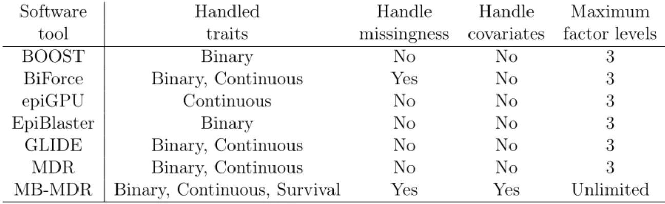
4) Provide a versatile software package that allow researchers to work with binary, continuous and survival traits, on datasets that may contain missing values, to consider multi-allelic data and categorical environmental exposure variables, to correct for main effects, regress covariates, correct for confouding factors, etc. Among the numerous software designed for pairwise or higher-order SNP-SNP inter-actions, we consider BOOST [131], BiForce [45], epiGPU [50], EpiBlaster [61], GLIDE [60], Multifactor Dimensionality Reduction (MDR) [101, 46] and Model-Based Multi-factor Dimensionality Reduction (MB-MDR) [13, 15]. Table 1.1 indicates which fea-tures related to our objectives are available in which software (without claiming to be exhaustive). Most methods do not handle missingness, but advocate to impute the missing data. In our lab, we advocate against imputing as such (without additional pruning steps) as it is known that linkage disequilibrium (LD) between markers can induce so-called redundant epistasis [87]. Two alleles at different loci are in LD if they occur together on the same chromosome more often than would be predicted by chance. Table 1.1: Available features in some common association interaction studies software

Software Handled Handle Handle Maximum

tool traits missingness covariates factor levels

BOOST Binary No No 3

BiForce Binary, Continuous Yes No 3

epiGPU Continuous No No 3

EpiBlaster Binary No No 3

GLIDE Binary, Continuous No No 3

MDR Binary, Continuous No No 3

(17)

Chapter 1

The following comparison of these approaches is mainly inspired from [43] which reviews and discusses several practical aspects GWAIs typically involve. BOOST is a software based on fast Boolean operations, to quickly search for epistasis associated with a binary outcome. Its main drawbacks are its limitation to binary traits, its inability to accommodate missing data and its necessity to perform a multiple testing

correction outside the software package. However, note that there is a module in

PLINK to deal with BOOST in a more flexible, but still not perfect way. BiForce is a regression-based tool handling binary and continuous outcomes, that can take account of missing genotypes and has a built-in multiple testing correction algorithm. However, the latter is based on a fast Bonferroni correction implementation, which leads to reduced power for GWAIs (this subject will be deeply discussed in Chapter 3). EpiBlaster, epiGPU and GLIDE are all GPU-based approaches. An obvious draw-back of GPU-dependent software is that it is tuned for a particular GPU-infrastructure. Therefore, users are advocated to acquire the exact same infrastructure and only ex-perts can adapt the code to specific needs. Note that users willing to work on dedicated hardware to speed up the computations can even turn to field-programmable gate array (FPGa) [137].

MDR is a non-parametric alternative to traditional regression-based methods that converts two or more variables into a single lower-dimensional attribute. The end goal is to identify a representation that facilitates the detection of linear or non-additive interactions. Over-fitting issues in MDR are solved via cross-validation and permutations. Since the design of MDR, several adaptations have been made [127].

MB-MDR breaks with the tradition of cross-validation and invests computing time in permutation-based multiple multilocus significance assessments and the implemen-tation of the most appropriate association test for the data at hand. It is able to correct for important main effects. Its main asset compared to the other methods is its versatility. MB-MDR can for instance be used to highlight gene (GxG), gene-environment (GxE) or gene-gene-gene-environment (GxGxE) interactions in relation to a trait of interest, while efficiently controlling type I error rates and false positives. The trait can either be expressed on a binary or continuous scale, or as a censored trait. Before the start of this thesis in 2011, the only available software implementing the MB-MDR methodology was a very slow R-package [12].

In this PhD, we propose a C++ implementation of the MB-MDR methodology, ful-filling the aforementioned four objectives. The latest version, mbmdr-4.4.1.out, can be downloaded at http://www.statgen.ulg.ac.be, with the associated documentation. Older versions are also still available. mbmdr-4.4.1.out is an easy to use command-line software, including a man-like help. To see its home page, use the following command: ./mbmdr-4.4.1.out help

In Chapter 2, we introduce our epistasis detection methods. In other words, the aim of this chapter is to answer the research question “How strongly is a particular GxG, GxE or GxGxE interaction related to the disease under investigation?”. This chapter successively describes the cases of a trait expressed on a binary scale, on a continuous scale and as a censored trait. Each time, methods are given for computing a number, called MB-MDR statistic, representing the degree of association between the interaction and the trait. These methods can be split into two categories: with and without correction for lower order effects.

(18)

Chapter 1

Chapter 3 addresses the multiple testing problem. In other words, it answers the research question “Correcting for the fact that a huge set of GxG, GxE or GxGxE interactions is investigated, what is the probability that a particular interaction is not significantly associated to the disease?”. This chapter is the corner stone of this PhD thesis. In particular, it contains a presentation of three classical multiple-testing correc-tion algorithms, Bonferroni, maxT and minP [39], but proposes new ways to implement them in order to reach better performances. The purpose of these three algorithms is to control the family-wise error rate (FWER), Bonferroni being the most conservative correction method. MaxT, the default algorithm used in the MB-MDR framework, has requirements in terms of computing time and memory proportional to the number of permutations. This makes it unsuitable for GWAIs. The first main contribution of this PhD thesis solves the memory issue: Van Lishout’s implementation of maxT makes the memory usage independent from the size of the dataset [125]. The second and most important contribution, gammaMAXT, solves the computing time issue: it speeds up the computing time further, while still controlling the FWER strongly and displaying a power similar to the original maxT algorithm.

Chapter 4 addresses the issue of population stratification and also discusses co-variate adjustments. Two new algorithms, STRAT1 and STRAT2, are introduced to automatically correct for unmeasured confounding factors. Furthermore, better per-formances can be observed by correcting for covariates. In this context, two strategies are presented to correct for covariates. Residuals-based correction is a simple method, whose computing time is almost the same as if no correction for covariates would be performed, that increases the power to detect significant interactions when a clear rela-tionship between the trait and the covariates that are regressed out exists. On-the-fly correction is a more computational intensive method, that allows to correct for any combination of categorical covariates and main effects of the SNPs, i.e. find out “pure” biological interactions that are not driven by any available variable.

Chapter 5 presents different applications of the software, both on simulated and real-life datasets. This chapter demonstrates that the software can be used successfully to either retrieve known interactions from the literature or find new ones. A lot could be learned from the data analysis performed in this chapter, leading to recommendations for the users of our software, as well as new insights into the assets and limitation of the methods developed in this PhD work.

(19)

Chapter 2 Epistasis detection

2.1 Outline

Epistasis is important to tackle complex human disease genetics [78]. It can be viewed from two perspectives, biological and statistical, illustrated in Figure 2.1. Biological epistasis is “the result of physical interactions among bio-molecules within gene regula-tory networks and biological pathways in an individual such that the effect of a gene on a phenotype depend on one or more other genes” [87]. Statistical epistasis is defined as “deviation from additivity in a mathematical model summarizing the relationship between multilocus genotypes and phenotypic variations in a population” [87].

Source: http://www.nature.com/ng/journal/v37/n1/fig_tab/ng0105-13_F1.html

Figure 2.1: Biological epistasis is defined at the individual level and involves DNA sequence variations (vertical bars), bio-molecules (square, circle and triangle) and their physical interactions (dashed lines), leading to a phenotype (star) [87]. Statis-tical epistasis is defined at the population level, as a phenomenon made possible by inter-individual variability in genotypes, bio-molecules and their interactions [87].

Writing a software that detects statistical epistasis is a challenging task. A typi-cal genome-wide real-life dataset is composed of millions of SNPs, leading to a huge amount of interactions to investigate, even when restricting our attention to two-order

interactions (in this case about 1012 _{SNPs). In this chapter, we specify our}

method-ology to compute an MB-MDR statistic, capturing the degree of association between a particular pair of SNPs and the trait. This enables to produce a ranking of the most promising interactions. In Chapter 3, we show how to compute a p-value indicating if a pair is statistically significantly associated to the trait or not.

(20)

Chapter 2 2.1 Outline

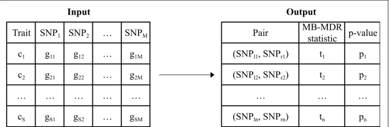
Figure 2.2 describes the input information that we have and the output that we aim to produce1_. Trait SNP1 SNP2 … SNPM MB-MDR statistic p-value c1 g11 g12 … g1M (SNPl1, SNPr1) t1 p1 c2 g21 g22 … g2M (SNPl2, SNPr2) t2 p2 … … … … cS gS1 gS2 … gSM (SNPln, SNPrn) tn pn Pair Input Output

Figure 2.2: The input information consists of the trait and SNP values for the S subjects under study. The trait can either be expressed on a binary or continuous scale, or as a censored trait (in the latter case the trait column is replaced by two columns, respectively for the time and censoring variables). In the event of a binary scale, if the sth subject is a case (control), cs = 1(0) (s = 1 . . . S). In the

case of a continuous scale, cs is a continuous value representing the state of the sth

subject. SN Pb is a label referring to the bth SNP (b = 1, . . . M ). The genotype of

an individual s at locus b is denoted as gsb (0 if homozygous for the first allele, 1 if

heterozygous, 2 if homozygous for the second allele and -9 if missing). Multi-allelic variables and categorical environment variables are also covered, as long as they are coded with natural numbers. The task consists in generating a ranking of the most significant SNP pairs in relation with the trait. (SNPlj, SNPrj) refers to the

jth _{best SNP pair, i.e. the pair with the j}th _{highest MB-MDR statistic t} j.

In this chapter, we propose different strategies for computing an MB-MDR statistic. Obviously, the scale of the trait leads to different types of statistics. Furthermore, miss-ing values in the dataset can be handled in different ways. Nonetheless, an important aspect is also whether to adjust the statistic for the main effect of the SNPs or not. It comes without saying that not adjusting leads to simpler statistics, faster to compute. However, as soon as the data contains at least one SNP with an important main effect, these statistics are not good enough. Indeed, the output would undoubtedly contain a lot of significant pairs, making it impossible to distinguish between real pure epistatic effects and results driven by the main effect. The default option in our software is thus to always adjust for main effects. We show in this chapter that there are several ways to perform the adjustment and discuss the benefits and drawbacks of each choice. In the next section, we focus on the scenario where the trait is expressed on a binary scale. We show how to compute a simple statistic (not adjusting for main effects) using the MB-MDR framework and how to compute two more elaborate statistics to regress the main effects. We also discuss the pros and cons of using other approaches from the literature. Traits expressed on a continuous and on a survival scale are handled in Sections 2.3 and 2.4.

1 _{In this document, we assign index 1 to the first element of a sequence to facilitate reading. However,}

(21)

Chapter 2 2.2 Binary traits

2.2 Trait expressed on a binary scale

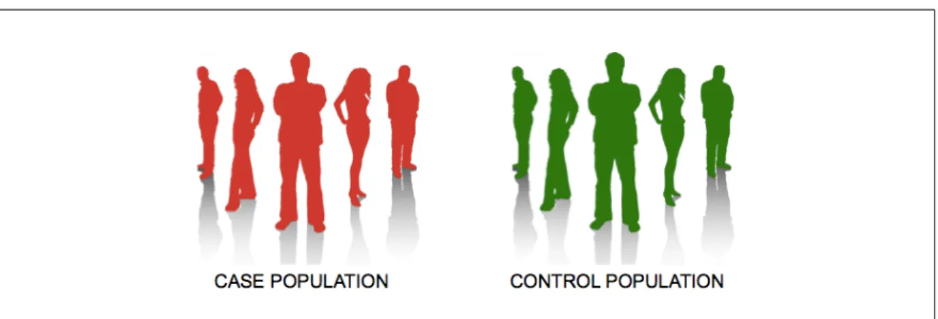
Case-controls studies are widely used in medicine. Typically, a group of patients having a disease (the “cases”) is compared to a group of patients not affected by the disease (the “controls”), as illustrated in Figure 2.3. This design does not factually restrict to diseased versus healthy patients. It can in general be used to split subjects in two groups depending on any condition (for instance, in the context of BMI, morbid obese or not). In this work, we are interested in finding the pairs of SNPs and/or environmental variables that bests predict the status of the subjects.

Figure 2.3: The aim of case-control studies is to determine if there is a statistically significant difference between the affected and unaffected subjects. In this thesis, we focus on genetic interactions that might regulate the susceptibility to the disease.

Our aim is to compute, for every pair [SNPlj, SNPrj], a number tj capturing its

degree of association with the trait. This allows to sort the pairs by decreasing chances of regulating the disease. Let N1 be the number of possible values for SNPlj and N2

the number of possible values for SNPrj. In practice, most of the studies concern

bi-allelic SNPs and N1 = N2 = 3. However, the software described in this thesis

automatically detects the exact values of N1 and N2, so that multi-allelic markers

(such as microsatellites) are also covered. Furthermore, environment variables can be also used as hypothesis, instead of SNPs, as long as they can be treated as categorical. They should be coded 0, 1, . . . , N1− 1, resp. 0, 1, . . . , N2− 1, in any convenient order.

2.2.1 Without correction for main effects

The MB-MDR framework proposes a slightly elaborate way to compute a statistic tj

representing the strength of the association between the pair [SNPlj, SNPrj] and the

trait T . In the discussion section at the end of this chapter, we discuss the pros and cons of taking a more direct approach, based on information theory. Since the MB-MDR method comes from its ancestor MB-MDR, we first present the latter. The idea of the MDR methodology, is to split the subjects into groups, depending on their genotypes. In the case of bi-allelic genetic marker, there are nine possible groups, as illustrated in Figure 2.4, inspired from [102]. Every non-empty group is either labeled “L” if it contains more controls than cases (low-risk) or “H” otherwise (high-risk). In this way, the dimensionality has been reduced to one dimension with two levels. However, note that although the dimension has been reduced, the effective degrees of freedom may not. It has been estimated to be 5.6 for MDR in case of interactions of order two [91].

(22)

Figure 2.4: In the MDR methodology, the subjects are split into groups depending on their genotypes. These multifactor classes can be organized in a matrix repre-sentation. For every subject, the alleles of SNPlj defines to which column it belongs

to and the alleles of SNPrj to which line. In every cell, the amount of cases is

re-ported on the left and the amount of controls on the right. If the controls represent the majority, the group is considered to be in low risk for the disease (in this work such cells are colored in green). Otherwise, the group is considered to be in high risk for the disease (in this work such cells are colored in orange). Empty cells are ignored. Pooling all the orange cells together and all the green ones together, forms the genetic model of the effect of the pair of SNPs on the disease.

A classical 10-fold cross-validation procedure is used to compute the cross-validation consistency and the prediction error [101]. The entire procedure is performed 10 times, to diminish the odds of observing false results due to a poor division of the subjects. The cross-validation consistency has to be maximized and is defined as “a measure of the number of times a particular set of loci and/or factors is identified across the cross-validation subset” [101]. The prediction error has to be minimized and is defined as “the average of prediction errors across each of the 10 cross-validation subsets” [101]. When the optimal is different among these two metrics, the simplest model is chosen. An important benefit of MDR is that it is a model-free approach. It does neither assume any particular genetic model, nor estimate any parameter. The dimensionality problem involved in interaction detection is tackled by pooling the subjects into two groups (“H” or “L”), hence the name of the method. Furthermore, this methodology does not just produce a list of pairs possibly linked to the trait, it also returns the corresponding genetic models of the disease. Empirical and theoretical studies suggest that MDR has excellent power for identifying epistasis [101].

(23)

An important drawback of this approach, it that the groups are forced to be either in high-risk or low-risk, even when there is no statistically significant difference between the amount of cases and controls [11]. Another hindrance is that the original method can only handle traits expressed on a binary scale, not a continuous one. The major drawback however, is probably that it cannot correct for the main effects of the SNPs, i.e. the effect that the SNPs have on their own on the trait. Therefore, we turn to the MB-MDR approach in this thesis, resolving all the aforementioned issues.

The idea of the MB-MDR methodology, is to split the subjects into groups in the same way as in the MDR methodology, except that there are now three possible categories instead of two: “O” if there is no statistical evidence for any risk change (neither high-risk, nor low-risk) and “L” or “H” otherwise, as illustrated in Figure 2.5.

Figure 2.5: In the MB-MDR methodology, the subjects are still split into groups depending on their genotypes, in the same way as in Figure 2.4. However, there are now three possible categories for the cells. A group is immediately assigned to the “O” category (no-evidence for any risk change) if it consists of less than ten individuals. Otherwise, a statistical test is performed to decide if there is a statistically significant difference between the number of cases and controls. If there is, the group is assigned to either the “H” or “L” category, in the same way as before. Otherwise, it is assigned to the “O” category (in this work such cells are colored in blue).

(24)

Figure 2.6 explains the computation of a statistic tj representing the strength of

the association between the pair [SNPlj, SNPrj] and the trait T .

Trait SNPlj SNPrj c1 g1lj g1rj c2 g2lj g2rj … … … cS gSlj gSrj A00 … A0(N2-1) U00 … U0(N2-1) … … … … A(N1-1)0 … A(N1-1)(N2-1) U(N1-1)0 … U(N1-1)(N2-1) R00 … R0(N2-1) … … … R(N1-1)0 … R(N1-1)(N2-1) tj

affected-subjects matrix unaffected-subjects matrix

HLO matrix

Figure 2.6: Computation of an MB-MDR statistic for a binary trait, without cor-rection for main effects. Input: cs is 1 (0) if the sth subject is a case (control),

gslj and gsrj are the genotypes of the sth subject for SNPlj and SNPrj respectively.

The computation can be decomposed in three steps. First, the affected-subjects

and unaffected-subjects matrices are constructed. Amn and Umn are respectively

the number of affected/unaffected subjects, whose genotype gslj = m and gsrj = n.

Second, the HLO matrix is constructed. Rmn is either “H” if the subjects whose

genotype is m for SNPlj and n for SNPrj have a high statistical risk of disease, “L”

if they have a low statistical risk and “O” if there is no statistical evidence (or no data). Third, the final tj value is computed from the three matrices constructed at

(25)

The three steps of the computation of the number tj capturing the degree of

asso-ciation between the pair [SNPlj, SNPrj] and the trait T are as follows:

1) Generation of the affected-subjects and unaffected-subjects matrices A and U . For efficiency reasons and to take account of empty groups more easily, these

objects are in fact coded as vectors2_{. They are created with a size N}

1 × N2

and initialized with zero values. Then, a loop over the subjects of the dataset is performed. For s = 1, . . . S: if no value is missing for subject s: increment a cell of the affected-subjects vector if cs = 1, otherwise a cell of the

unaffected-subjects one. The index of the cell to be incremented is given by gslj× N2+ gsrj,

i.e. depends on the subject’s genotype3. The total amount NAof affected and NU

of unaffected subjects without missing values can easily be deduced from these vectors. After this process, a loop is performed to create a vector T containing the total number of subjects in each non-empty group and a vector Y containing

the ratio of cases versus number of subjects in each non-empty group4_{. Empty}

groups are removed from A and U on the fly during this process. Let dim be the final size of vectors A, U , T and Y .

2) Generation of the HLO-matrix from the objects generated at step 1. This object is in fact also coded as vector for efficiency reasons and has a size of dim. Each Rh

element depends on a test for association between the trait and the belonging to the genotype group satisfying (SNPlj×N2+SNPrj = h), with h = 0, . . . , dim−1.

A χ2_{test with one degree of freedom (1 df) is performed by default, to keep things}

simple. However, the architecture of the software makes it easy to implement other test statistics that are appropriate for the data at hand. The statistic that we use follows a χ2 distribution and is defined as _{(a+b)(c+d)(b+d)(a+c)}(ad−bc)2(a+b+c+d) , where a (c) refers to the number of affected (unaffected) subjects having a genotype satisfying (SNPlj× N2+ SNPrj = h) and b (d) refers to the number of affected (unaffected)

subjects having a different genotype. Those values are easy to compute: a = Ah,

b = NA− Ah, c = Uh and d = NU − Uh. At this point, if either a + c or b + d

is below a threshold that is a parameter of the program (default value 10) then the test is not performed at all, since it would not be statistically significant. In this case the value of Rh is automatically set to “O”, to indicate the absence

of evidence that the subset of individuals with multilocus genotype satisfying SNPlj× N2+ SNPrj = h has neither a high nor a low risk for disease. Otherwise,

the test is performed. When the computed χ2

obs value is below the critical value5

χ2_crit = 2, 705543, the value of Rh is set to “O”, to indicate that we cannot reject

the independence hypothesis. Otherwise, Rh is set to either “H” if (ad − bc) > 0,

to indicate a high risk of having the trait, or to “L” if (ad − bc) < 0, to indicate a low risk for this event.

2 _{From the programmers perspective, coding a matrix as a vector is just an implementation choice.}

Matrices are used in Figure 2.6 because from a conceptual point of view it is easier to understand.

3 _{Note that this is the same as working in matrix format and numbering the cells from left to right}

and top to bottom, by starting with 0 on the top left corner and finishing on the bottom right one.

4 _{The vectors T and Y are not necessary from a conceptual point of view (they can be deduced from}

A and U ) and do therefore not appear in Figure 2.6. In practice, they are useful to win computing time by avoiding some operations to be performed several times in the next steps.

(26)

3) Computation of tj from the objects generated at steps 1 and 2. It consists in

performing two χ2 _{tests with 1 df and returning the maximum of both. The first}

one tests association between the trait and the belonging to the “H” category versus the “L” or “O” one. The second one tests association between the trait and the belonging to the “L” category versus the “H” or “O” one. In the first (second) case, a and c are respectively the number of affected and unaffected subjects belonging to the “H” (“L”) category and b and d to the “L” (“H”) or “O” category. Computing this can easily be achieved by initializing a, b, c and d to zero, and for h = 0, . . . , dim − 1 adding Ah to a and Uh to c if Rh = “H” (“L”)

and Ah to b and Uh to d otherwise. Note that in many case, there are only cells

associated to the “O” category and tj is readily equal to zero.

The detailed algorithm computing statistics tj (without correction for the main

effects of the SNPs) is reported in Box 2.1.

Box 2.1. Binary MB-MDR statistic computing (no 1st _{order correction)}

(1) Create vectors A, U , T and Y of size dim = N1×N2. Define χ2crit= 2, 705543.

(2) Fill A and U with 0’s. For s = 1, . . . , S: if gslj and gsrj are not missing do

either Agslj×N2+gsrj++ if cs = 1 or Ugslj×N2+gsrj++ otherwise.

(3) Set a = 0. For h = 0, . . . , dim − 1: compute Ta= Aa+ Ua ; if (Ta = 0) erase

the ath element of vectors A and U , else compute Ya = A_T_aa and perform a++.

After the loop compute the final dimension: dim = a.

(4) Compute NA = A0+ . . . + Adim−1, NU = U0+ . . . + Udim−1 and N = NA+ NU.

(5) Create HLO vector R of size dim. For h = 0, . . . , dim − 1: (a) Define a = Ah, b = NA− a, c = Uh and d = NU − c.

(b) If (a + c) < 10 or (b + d) < 10: set Rh = “O”, else compute

χ2_obs = _N (ad−bc)2N

ANU(b+d)(a+c). If χ

2 obs < χ

2

crit set Rh = “O”, else if

(ad − bc) < 0 set Rh = “H”, else set Rh = “L”.

(6) If there is no “H” and no “L” in the R vector, return tj = 0.

(7) If there is at least one “H”:

(a) Initialize a = 0 and c = 0. For h = 0, . . . , dim − 1: if Rh = “H” compute

a+=Ah and c+=Uh.

(b) Define b = NA− a and d = NU− c. Compute χ2HvsLO =

(ad−bc)2_N

NANU(b+d)(a+c).

(8) If there is at least one “L”:

(a) Initialize a = 0 and c = 0. For h = 0, . . . , dim − 1: if Rh = “L” compute

a+=Ah and c+=Uh.

(b) Define b = NA− a and d = NU− c. Compute χ2LvsHO =

(ad−bc)2_N

NANU(b+d)(a+c).

(27)

Since we are interested in GWAIs and GWEIs, we must realize that the part of the code that reads the data at the start of the program cannot store it in cache because of its size. Accessing to the trait and SNP values is thus slow and must be avoided

as much as possible. For this reason, the three columns Trait , SNPlj and SNPrj of

Figure 2.6 are passed by value and not by reference to the function. In this way, an explicit local copy of them is performed, on which the function is able to work faster. Note that the loops at step (3), (4), (5), (7) and (8) in Box 2.1. involves only up to nine iterations (in the bi-allelic case) and are therefore very fast. Everything has been optimized to reduce the number of operations to a minimum. This is indeed crucial, since this function is called about 1015 _{times for GWAIs, as shown in Chapter 3.}

An important benefit of MB-MDR, is that the robust association tests that are performed, hereby acknowledging that not all multi-locus genotype combination are informative, have proven to give optimal performance compared to MDR, especially in the presence of genetic heterogeneity [15]. Another value of MB-MDR is that it is flexible: it can be adapted to correct for the main effects of the SNPs in different ways, it can handle missingness optimally, the trait can be expressed on different scales,... The main drawback of the computation of MB-MDR statistics compared to MDR ones, is that they require more computing time. However, by optimizing all steps as we did, the calculation time can be kept low (numerical results are given in Chapter 3).

2.2.2 With correction for main effects

In the previous section, we have shown strategies to perform a global epistasis test. In this section, we show how to perform a targeted epistasis test within the MB-MDR framework, by adjusting for lower-order effects. This is in fact the origin of the model-based (MB) component in the name of the MB-MDR methodology. Correcting for lower-order effects avoids main effects signals giving rise to false epistasis effects [80]. Coding scheme

In genome-wide association testing, the SNPs are often coded in an additive way, i.e. the code is given by the number of minor alleles [38]. For instance, if A is the major allele and C the minor one, AA is coded 0, AC is coded 1 and CC is coded 2. If C has a negative effect on the disease, the genotype CC is considered to be two times worse for the subject’s health than the AC one. The additive scheme is very straightforward and can work well in a lot of scenarios, but power can be gained by taking the true underlying genetic models into account [108]. An alternative is to use a codominant coding. In the bi-allelic case, two binary variables are used: one equal to 1 for AC and 0 otherwise and the other equal to 1 for CC and 0 otherwise. In mbmdr-4.4.1.out, the user can choose between these two coding. Codominant is the default, since it is an all-purpose acceptable (in terms of power and type I error) choice [79]. In practice, choosing between additive and codominant coding schemes implies choosing between the least and most severe such removal of effects [79]. The general idea of the lower-order correction is as follows. First, construct the affected-subjects and unaffected-subjects matrices of Figure 2.6, but implemented as vectors. Then, create again a vector Y of size dim containing the ratio of cases versus number of subjects for every non-empty group. Then, try to fit the following model:

(28)

where X is the model matrix and β a row vector of parameters to fit. For an additive correction, the model matrix Xadditive consists of dimc = 3 columns (one for

the intercept, 1 for SNPlj and 1 for SNPrj) and dim rows [14]. The second column

corresponds to the value of SNPlj and the third one to the value of SNPrj . Vector β

is obviously composed of dimc = 3 elements. In the bi-allelic case, when no group is

empty, the model matrix is given explicitly by

Xadditive =               1 0 0 1 0 1 1 0 2 1 1 0 1 1 1 1 1 2 1 2 0 1 2 1 1 2 2               (2.2)

For a codominant main effects correction, the model matrix Xcodominant consists of

dimc= N1 + N2− 1 columns (one for the intercept, N1− 1 for SNPlj and N2− 1 for

SNPrj) and dim rows [14]. Vector β is obviously composed of dimc = N1 + N2 − 1

elements as well. In the bi-allelic case, the second (third) column is 1 if SNPlj has

value 1 (2) and 0 otherwise and the fourth (fifth) column is 1 if SNPrj has value 1 (2)

and 0 otherwise. In this case, when no group is empty, the matrix is given by

Xcodominant=               1 0 0 0 0 1 0 0 1 0 1 0 0 0 1 1 1 0 0 0 1 1 0 1 0 1 1 0 0 1 1 0 1 0 0 1 0 1 1 0 1 0 1 0 1               (2.3)

When a group is empty, the corresponding row is removed from X and the corre-sponding element from Y . This process can produce a model matrix that is singular. Trying to fit the model would fail. An obvious way to avoid this would be to check if the matrix is singular or not and act accordingly. However, in practice the matrix is almost never singular and testing the singularity each time would lead to a big waste of time. For this reason, the code is organized as a “try and catch” block. First, the software tries to estimate the model without taking care of this issue. Then, in the rare cases where it fails, the matrix is investigated in details and the linearly dependent columns are removed. From a programming point of view, it is important to realize that the model matrix is strictly the same for most of the SNP pairs. Indeed, the majority of the SNPs are bi-allelic. For this reasons, the Xadditive and Xcodominant matrices are

hard-coded. In this way, significant computing time can be saved. When empty groups are present, the actual model matrix used is easy to construct from the hard-coded one, by keeping only the rows corresponding to the non-empty groups. When at least one SNP is not bi-allelic, the most common scenarios are again hard-coded and in the very rare other cases, the model matrix is constructed explicitly.

(29)

Fitting the model

This section is mainly influenced by [14]. The strategy to fit equation 2.1 is to start from an initial guess and to update it iteratively. This can be achieved using the Newton-Raphson method [19], since the Y vector contains expected outcome values and not binary ones. In fact, for generalized linear models (GLMs), this comes down to iteratively reweighted least squares (IRLS). The implementation is based on the R function glm.fit and described in Box 2.2.

Box 2.2. Model fitting using IRLS

(1) Create vectors A, U , T and Y of size dim = N1×N2. Define χ2crit= 2, 705543.

(2) Fill A and U with 0’s. For s = 1, . . . , S: if gslj and gsrj are not missing do

either Agslj×N2+gsrj++ if cs = 1 or Ugslj×N2+gsrj++ otherwise.

(3) Create matrix X consisting of dimc = 3 columns in case of additive coding

and dimc = N1 + N2− 1 columns in case of codominant coding. Set a = 0.

For h = 0, . . . , dim − 1: compute Ta = Aa+ Ua ; if (Ta = 0) erase the ath

element of vectors A and U , else perform the following operations

(a) Add the ath row of the hard-coded model matrix to X.

(b) Compute Ya = A_T_aa.

(c) Perform a++. Compute dim = a.

(4) Compute NA = A0+ . . . + Adim−1, NU = U0+ . . . + Udim−1 and N = NA+ NU.

(5) Create fitted values vector µ of size dim and initialize all elements to NA

N .

(6) Create linear predictor vector η = ln(_1−µµ ).

(7) Compute D = 2{N lnN −NAlnNA−NU lnNU+

dim−1

P

i=0

[Ailn(Yi)+Uiln(1−Yi)]}. (where only the first term of the latter sum is taken if Yi= 1 and only the second if Yi= 0)

(8) Perform the following iterations:

(a) Create a vector z = η +_µ(1−µ)Y −µ (taking zi= ηi− 1 if µi= 0 and zi= ηi+ 1 if µi= 1)

(b) Calculate the dim × dim diagonal matrix W where Wii = Tiµi(1 − µi).

(c) Calculate dimc× dimc symmetric positive definite matrix I = X0W X.

(d) Calculate the right-hand side vector v of size dimcdefined by v = X0W z.

(e) Calculate vector β of size dimc by trying to solve Iβ = v. If it fails,

remove all linearly dependent columns from X and go back to step (c). (f) Update η = Xβ and µ = _1+e1−η.

(g) Compute D = 2{

dim−1

P

i=0

Ai ln_µYi_i + Ui ln1−Y_1−µi_i).

(where only the first term is taken if Yi= 1 and only the second if Yi= 0)

(h) Stop iterating if |D−Dold|

0.1+D < 10

(30)

At step (5), the fitted values vector µ is initialized to the values under the null model (only intercept), i.e. the trivial model fit consisting of the observed ratios of cases versus individuals in each group. The difficult part is step (8) (e). Because I is symmetric and positive definite, this linear system can be solved based on the Cholesky decomposition of I, which is guaranteed to exist and be unique if X is not singular:

I = LDL0 (2.4)

where L is a dimc × dimc lower triangular matrix with diagonal elements equal

to 1 and D a dimc× dimc diagonal matrix with strictly positive diagonal elements.

The linear system Iβ = v can then be solved by subsequently solving Lv1 = v for v1,

Dv2 = v1 for v2 and L0β = v2 for β. Hence, no explicit matrix inversion is involved. In

practice, we call a library (alglib) that performs the Cholesky decomposition very fast. As already mentioned, this part of the code is organized as a try-catch block. Indeed, the decomposition can only fail if X is singular (which leads to a matrix I that is not positive definite) and in this case the linearly dependent columns are removed from X. Test statistic

So far, we have defined a model and have shown how to fit it. However, there was no obvious link to the MB-MDR methodology. The connection is in fact that, instead of performing simple χ2 tests as in steps (5), (7) and (8) of Box 2.1, score statistics are used to take account of the model. In each of these steps, the idea was to compare a selection of subjects S1 versus the others S0. At step (5), the subjects with one

particular genotype versus the rest. At step (7) (respectively 8), the subjects belonging to the “H” (respectively “L”) category versus the rest. To simultaneously take account of the main effects and of the group belongings, the model matrix needs to be extended. A column is added at the back of matrix X, whose value is 1 if the row corresponds to subjects belonging to S1 and 0 otherwise. To avoid confusion in the rest of this section,

we note Xmain the original model matrix (taking only the main effect into account)

and Xc+1 the aforementioned extra column. The score statistic is defined by

S = u

2

i (2.5)

where the score u and information i can be computed in different ways. A stable

calculation is based on the QR decomposition Q1R1 =

√

W Xmain [110]. This QR

decomposition is thin and needs to be executed only once. The extra column Xc+1

is explicitly orthogonalized with respect to Xmain by solving R1V = QT1

√

W Xc+1 for

vector V and calculating O = Xc+1− XmainV. From this, we can calculate

u =X i WiOiρi (2.6) i =X i WiOi2 (2.7)

where the residual vector ρ of size dim is given by

ρ = Y − µ

(31)

Algorithm

In the previous section, we have given all the pieces of the puzzle to compute a number tj, capturing the degree of association between the pair [SNPlj, SNPrj] and the trait T ,

adjusted for the main effects of the two SNPs (or environmental variables), using either a codominant or an additive coding scheme. In this section, we sum up everything and give the exact algorithm. The computation still follows the general scheme of Figure 2.6, but the three steps are now as follows:

1) The first step still begins by constructing the affected-subjects and unaffected-subjects matrices, but again coded as vectors. They are obtained in the exact same way as in Section 2.2.1. Then, vectors T and Y are again constructed, while adjusting the size of A and U to take account of empty groups, but with a small difference compared to Section 2.2.1: the model matrix X is as well constructed on the fly during this process as well. It is created empty and at each iteration h = 0, . . . , dim − 1, if there is at least one subject whose genotype

satisfies (SNPlj × N2 + SNPrj = h), the hth row of the hard coded-matrix is

added as the next row of X. Recall that in the rare cases where the hard-coded matrix does not exist, i.e. when either N1 > 3 or N2 > 3, then the row is created

explicitly. At the end of this step, A, U , T and Y contains dim elements and X contains dim rows, where dim is the number of non-empty groups.

2) The second step still consists in generating the HLO-matrix, but again coded in vector format. First, the model is fitted as described in Box 2.2 and the

QR decomposition Q1R1 =

√

W Xmain is obtained by calling a library (alglib)

dedicated for this task. Then, a column is added at the back of X. Each Rh

element of the HLO-vector depends on a test for association between the trait

and the belonging to the genotype group satisfying (SNPlj× N2+ SNPrj = h),

but this time adjusted for the main effects of the SNPs. For h = 0, . . . , dim − 1, if Th < 10 set the hth element of the HLO-vector to “O”. Otherwise, overwrite

the last column of X with 0’s, except the hth _{element which is set to 1. Then}

compute the score statistic from equation 2.5. When this value, following a 1df (one degrees of freedom) χ2, is below the critical value χ2_crit = 2, 705543, set the hth _{element of the HLO-vector to “O”. Otherwise, set it to either “H” if u > 0 or}

“L” otherwise.

3) If there is neither “H” nor “L” values in the HLO vector, return 0. Otherwise, compute the following two score statistics. First, overwrite the last column of X with 0’s, except for the elements for which the corresponding element of the HLO vector is equal to “H” which are set to 1. Then, compute the score statistic from equation 2.5. Second, do exactly the same except that the elements set to 1 are now those corresponding to a “L” value. Of course, if there are no “H” (“L”) values, the first (second) number is not computed and the functions obviously returns the second (first) one. Otherwise, the function returns the maximum of the two numbers.

(32)

Box 2.3. Binary MB-MDR statistic computing (with 1st _{order correction)}

(1) Execute the algorithm from Box 2.2. Find Q1R1 =

√ W X.

(2) Create empty vectors V of size dimcand O of size dim. Create residual vector

ρ of size dim. For i = 0, . . . , dim − 1: if (µi = 0) set ρi = −1, else if (µi = 1)

set ρi = 1, else set ρi = _µY_i_(1−µi−µi_i₎.

(3) Create empty HLO vector R of size dim. For h = 0, . . . , dim − 1: (a) If (Th < 10) set Rh = “O” and skip steps (b), (c), and (d).

(b) For j = 0, . . . , dimc−1: execute Vj = Q1hj

√

Wh. For i = dimc−1, . . . , 0:

do (for j = i + 1, . . . , dimc− 1: Vi = Vi− R1ijVj) and (Vi = _RV_1iii ).

(c) For s = 0, . . . , dim − 1: do (Os = 0) and (for t = 0, . . . , dimc − 1:

Os = Os− XstVt). Execute Oh++.

(d) Set u = i = 0. For s = 0, . . . , dim − 1: do (u+=WsOsρs) and

(i+=WsOs2). If i=0 set Rh = “O”, else calculate S = u

2

i . If S < χ 2 crit set

Rh = “O”, else if (u > 0) set Rh = “H”, else set Rh = “L”.

(4) If there is no “H” and no “L” in the HLO vector R, return tj = 0.

(5) If there is at least one “H”:

(a) For i = 0, . . . , dimc − 1: do (Vi = 0) and (for j = 0, . . . , dim − 1: if

(Rj = “H”) do (Vi = Vi + Q1jipWj). For i = dimc− 1, . . . , 0: do (for

j = i + 1, . . . , dimc− 1: Vi = Vi− R1ijVj) and (Vi = _RV_1iii ).

(b) For s = 0, . . . , dim − 1: do (if (Rj = “H”) do Os= 1 else do Os= 0) and

(for t = 0, . . . , dimc− 1: do Os = Os− XstVt).

(c) Set u = i = 0. For s = 0, . . . , dim − 1: do (u+=WsOsρs) and

(i+=WsOs2). If (i>0) compute SHvsLO = u

2

i else set it to zero.

(6) If there is at least one “L”:

(a) For i = 0, . . . , dimc − 1: do (Vi = 0) and (for j = 0, . . . , dim − 1: if

(Rj = “L”) do (Vi = Vi+ Q1jipWj). For i = dimc− 1, . . . , 0: do (for

j = i + 1, . . . , dimc− 1: Vi = Vi− R1ijVj) and (Vi = _RV_1iii ).

(b) For s = 0, . . . , dim − 1: do (if (Rj = “L”) do Os = 1 else do Os= 0) and

(for t = 0, . . . , dimc− 1: do Os = Os− XstVt).

(c) Set u = i = 0. For s = 0, . . . , dim − 1: do (u+=WsOsρs) and

(i+=WsOs2). If (i>0) compute SLvsHO = u

2

i else set it to zero.

An efficient and flexible software tool for genome-wide association interaction studies

University of Liège

Faculty of Applied Sciences

Department of Electrical Engineering and Computer Science

Montefiore Institute

An Efficient and Flexible

Software Tool

for

Genome-Wide Association

Interaction Studies

-Academic year

2015-2016

PhD thesis by

Van Lishout François

Promotor

Jury members

Acknowledgements

Abstract

Résumé

Contents

List of Figures

List of Tables

List of Algorithms

Chapter 1

General introduction

Chapter 2

Epistasis detection

2.1

Outline

2.2

Trait expressed on a binary scale

2.2.1

Without correction for main effects

2.2.2

With correction for main effects