Energy management of a grid-connected
PV plant coupled with a battery energy
storage device using a stochastic approach
Jonathan Dumas°, Bertrand Cornélusse°, Antonello Giannitrapani*, Simone
Paoletti*, Antonio Vicino*
° Liège university, Local energy community, Belgium
* Dipartimento di Ingegneria dell’Informazione e Scienze Matematiche Universita` di Siena, Italy
Capacity firming context
System
->
PV/wind generation
+
energy storage system
Where ?
->
Remote areas
: French islands (Réunion, Corse, Guadeloupe, etc)
Goal
-> The
intermittent
power from a PV/wind plant has to be
maintained
at a
committed level
.
How ?
-> The
energy storage system
smoothes the output and controls the ramp
rate (MW/min).
Summary
1. Literature review
2. Capacity firming process
3. Problem formulation
4. Case study
5. Conclusions & perspectives
PMAPS 2020
Literature review: day ahead bidding
The optimal bidding strategies with only a
production device:
[1,2].
[1] P. Pinson, C. Chevallier, and G. N. Kariniotakis, “Trading wind generation from short-term probabilistic forecasts of wind power,” IEEE Transactions on Power Systems, vol. 22, no. 3, pp. 1148–1156, 2007.
[2] A. Giannitrapani, S. Paoletti, A. Vicino, and Zarrilli, “Bidding wind energy exploiting wind speed forecasts,” IEEE Transactions on Power Systems, vol. 31, no. 4, pp. 2647–2656, 2015.
Incorporating an
energy storage
and dealing with the
uncertainties
: SDDP/
SDP [3]/[4], chanced-constrained [5],
2-stage stochastic
[6], robust
optimization [7,8].
[3] M. V. Pereira, L. M. Pinto, Multi-stage stochastic optimization applied to energy planning, Mathematical programming 52 (1- 3) (1991) 359–375.
[4] P. Haessig, B. Multon, H. B. Ahmed, S. Lascaud, P. Bondon, Energy storage sizing for wind power: impact of the autocorre- lation of day-ahead forecast errors, Wind Energy 18 (1) (2015) 43–57.
[5] F. Conte, S. Massucco, F. Silvestro, Day-ahead planning and real-time control of integrated pv-storage systems by stochastic optimization, IFAC-PapersOnLine 50 (1) (2017) 7717–7723.
[6] A. Parisio, E. Rikos, L. Glielmo, Stochastic model predictive control for economic/environmental operation management of microgrids: An experimental case study, Journal of Process Control 43 (2016) 24–37.
[7] D. Bertsimas, E. Litvinov, X. A. Sun, J. Zhao, T. Zheng, Adaptive robust optimization for the security constrained unit commitment problem, IEEE transactions on power systems 28 (1) (2012) 52–63.
[8] R.Jiang, J.Wang, Y.Guan, Robust unit commitment with wind power and pumped storage hydro, IEEE Transactions on Power Systems 27 (2) (2011) 800–810.
Mixed integer quadratic programming, simulation-based genetic algorithm,
PMAPS 2020
Contributions: PMAPS 2020 paper + extension
2 layers approach:
-
2-stage stochastic planner scenario based approach -> day-ahead bidding;
-
deterministic controller -> real-time set points.
Formulation:
-
Mix Integer Quadratic Programming (MIQP);
-
linear constraints to approximate a non-convex penalty function,
compatible
with a
scenario approach.
PV scenarios:
-
Gaussian copula methodology based on the parametric PVUSA model using
a weather
regional climate model.
2-stage
stochastic planner vs deterministic counterpart:
Summary
1. Literature review
2. Capacity firming process
3. Problem formulation
4. Case study
5. Conclusions & perspectives
PMAPS 2020
Day ahead engagement process
Figure 1: Day ahead engagement process.
The engagement plan is accepted if it satisfies
the constraints
Dead line
Forecaster Planner
PV
BESS
Grid
Optimization over T periods
Revenue Cost
Real-time process
Figure 2: Real-time control process.
Forecaster
Controller
PV
BESS
Grid
Optimization over Z periods at t
Revenue
Cost
Planner
Monitoring
Penalty and revenue
Figure 3: Penalties (left) and net revenues (right).
Engagement = 50 % of PV installed capacity, deadband tolerance = 5%.
Summary
1. Literature review
2. Capacity firming process
3. Problem formulation
4. Case study
5. Conclusions & perspectives
PMAPS 2020
Formulation: day ahead nomination
The objective
deterministic
(D=S with one scenario) counterpart is
The objective
2-stage
stochastic
(S) programming using a
scenario
approach is
(3)-(4) are
Mix Integer Quadratic Problems
(MIQP). The S formulation uses
J
D
= ∑
τ∈𝒯
− Δ
τ
π
τ
p
τ
+ c(p
⋆
τ
, p
τ
) (4)
J
S
= ∑
ω∈Ω
α
ω
∑
τ∈𝒯
[− Δ
τ
π
τ
p
τ,ω
+ c(p
⋆
τ
, p
τ,ω
)] (3)
PMAPS 2020
Revenue
Penalty
Formulations: real-time control
The
oracle
(= D planner) assumes
perfect knowledge of PV and uses day
ahead
engagements as inputs
J
oracle
= ∑
t∈𝒫
− Δ
t
π
t
p
t
+ c(p
⋆
t
, p
t
) (5)
The
real-time controller
(RT) uses the
last PV measured value, the PV
point forecasts, and day ahead engagements, for t in [1, P]
J
RT
=
∑
t∈𝒫∖{1,...,t−1}
− Δ
t
π
t
p
t
+ c(p
⋆
t
, p
t
) (6)
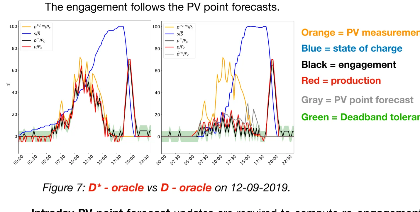
WARNING
: RT should use
intraday PV point forecasts updates to
Summary
1. Literature review
2. Capacity firming process
3. Problem formulation
4. Case study
5. Conclusions & perspectives
PMAPS 2020
The Uliège case study: dataset
Figure 4: PV max per day of the Liège dataset.
-
08-12/2019:
4 months
P
m
%,max
=
P
m
max
P
c
PMAPS 2020
PV scenarios
Red =
PVUSA point forecast
Black = PV
measurement
Grey = 5 PV scenarios
PVUSA:
NMAE = 4.25 %
NRMSE = 9.20 %
PMAPS 2020
Simulation parameters
BESS parameters:
-
capacity =
Pc * 1 hour = 466.4 kWh
-
charging and discharging efficiencies =
0.95
-
charging and discharging power =
Pc = 466.4 kW
-
initial state of charge =
0 kWh each day
-
state of charge of the last period =
0 kWh each day
Simulation parameters:
-
Pc =
466,4 kWp
-
Planning and controlling periods =
15 min
-
Peak hours:
7 - 9 pm
-
Selling price =
100 €/MWh (300 during peak hours)
-
Deadband engagement tolerance =
5 % Pc
-
Engagement ramping constraints =
7.5 % Pc/15min
PMAPS 2020
Computation times
Table 1: Computation times.
(s)
(s)
Solver & software:
-
Cplex (MIQP)
-
Pyomo python library
-
Ubuntu 18.04 LTS
-
Intel core i7-8700 3.20 GHz based
computer with 12 threads and 32 GB of
RAM
Day ahead engagement
computation time is not an issue.
Results
Table 3: Results.
S^20 and D
achieved similar results both with the oracle and RT controllers.
Table 2: Indicators.
Conclusions & extensions
The
2-stage stochastic approach achieved similar results than its
deterministic counterpart.
-> At least
one full year of data are required to produce « good » PV
scenarios (seasonality).
->
Intraday weather forecast updates are required to compute
re-engagements and run « properly » the
RT controller.
-> Extension to a
robust formulation
is currently underwork using
quantile PV generation forecasts.
Annex
1. Weather forecasts
2. PV point forecasts
3. PV scenarios
Weather forecasts: MAR regional climate model
Figure 6a: Irradiation.
Figure 6b: Air temperature.
PV point forecasts
PV point forecasts
are computed using the
PVUSA model
[10] which
expresses the instantaneous generated power as a
function of irradiance
and air temperature according to the equation
[10] R.Dows, E.Gough, PVUSA procurement, acceptance, and rating practices for photovoltaic power plants, Tech. Rep., Pacific Gas and Electric Co., San Ramon, CA (United States). Dept. of ..., 1995.
The PVUSA parameters (a, b, and c) are estimated following the algorithm of
[11].
Weather forecasts are provided by the Laboratory of Climatology of
the university of Liège, based on the
MAR regional climate model
[12],
http://climato.be/cms/index.php?climato=fr_previsions-meteo.
[11] G.Bianchini, S. Paoletti, A. Vicino, F. Corti, F. Nebiacolombo, Model estimation of photovoltaic power generation using partial information, in: IEEE PES ISGT Europe 2013, IEEE, 1–5, 2013.
[12] X. Fettweis, J. Box, C. Agosta, C. Amory, C. Kittel, C. Lang, D. van As, H. Machguth, H. Galle ́e, Reconstructions of the 1900–2015 Greenland ice sheet surface mass balance using the regional climate MAR model, Cryosphere (The) 11 (2017) 1015–1033.
̂P = a ̂I+ b ̂I
2
+ c ̂I ̂T (7)
PMAPS 2020
PV scenarios
The Gaussian copula methodology has already been used to generate wind
and PV scenarios in, e.g., [13,16].
This approach is used to
sample PV error scenarios
(Z) based on a point
forecast model.
[13] P. Pinson, H. Madsen, H. A. Nielsen, G. Papaefthymiou, B. Klöckl, From probabilistic forecasts to statistical scenarios of short-term wind power production, Wind Energy: An Inter- national Journal for Progress and Applications in Wind Power Conversion Technology 12 (1) (2009) 51–62.
[14] P.Pinson,R.Girard, Evaluating the quality of scenarios of short-term wind power generation, Applied Energy 96 (2012) 12–20.
[15] G. Papaefthymiou, D. Kurowicka, Using copulas for modeling stochastic dependence in power system uncertainty analysis, IEEE Transactions on Power Systems 24 (1) (2008) 40–49.
[16] F. Golestaneh, H. B. Gooi, P. Pinson, Generation and evaluation of space–time trajectories of photovoltaic power, Applied Energy 176 (2016) 80–91.