Volatility as an Asset Class for Long-Term Investors

Volatility as an Asset Class for Long-Term Investors

M. Brière

, A. Burgues

and O. Signori

13 April 2009

Abstract

This work shows how long-term investors can benefit from adding volatility as an asset class to their portfolio. Two types of "structural" exposure – long implied volatility and long volatility risk premium – are now simple to implement. Implied volatility exposure can be used to significantly reduce the risk profile of the portfolio, and especially extreme risks. Adding a volatility risk premium investment is less appealing: it substantially increases returns for a given level of risk, but at the cost of higher extreme risks. However a combination of the two volatility strategies is very attractive, thanks to fairly effective reciprocal hedging during periods of market stress. It delivers enhanced absolute and risk-adjusted returns, with smaller extreme risks than a traditional portfolio. Over the long term, volatility strategies make it possible to build portfolios that are more efficient than a pure-bond or equity/bond investment.

1

Centre Emile Bernheim Solvay Business School Université Libre de Bruxelles Av. F.D. Roosevelt, 50, CP 145/1 1050 Brussels, Belgium.

2

Crédit Agricole Asset Management, 90 bd Pasteur, 75015 Paris

*Comments could be sent to marie.briere@caam.com, alexandre.burgues@caam.com, or ombretta.signori@caam.com. The authors are grateful to A. Berkelaar, E. Bourdeix, T. Bulger, F. Castaldi, J. Coche, A. Drew, B. Drut, L. Dynkin, C. Guillaume, B. Houzelle, S. de Laguiche, K. Nyholm, A. Reveiz, A. Szafarz, K. Topeglo and the participants of the BIS/ ECB/World Bank Public Investors Conference 2008 for helpful comments and suggestions.

1. INTRODUCTION

Long-term investors are usually very conservative in their asset allocations, investing the bulk of their portfolios in government bonds. What often deters them from including other assets is inherent portfolio risk. Many long-term investors, such as pension funds and sovereign wealth funds, have substantial liabilities that prevent them from making risky allocations. By opting for conservatism, however, they are also denying themselves the opportunity to invest in asset classes that earn higher returns over the long run.

Volatility can be considered as a full-fledged asset class with many advantages. For example, being negatively correlated with equities, it can reduce the risk of an equity investment without sacrificing returns. But the advantages of volatility do not stop there. The recent development of standardized products, especially volatility index futures and variance swaps, gives investors access to a wide range of strategies for gaining structural exposure to volatility.

Two sets of strategies can be used to gain volatility exposure, namely long investment in implied volatility and long exposure to the volatility risk premium. The latter is the difference between the implied volatility of an underlying and its subsequent realized volatility. Though very different, the two strategy sets are consistent with the classic motivations –diversification and return enhancement – that prompt investors to opt for an asset class. Being long implied volatility seems to be compelling to investors for diversification purposes (Daigler and Rossi (2006), Dash and Moran (2005)). The remarkably strong negative correlation between implied volatility and equity prices during market downturns offers timely protection against the risk of capital loss. It has been well-documented in the academic literature (Turner et al. (1989), Haugen et al. (1991), Glosten et al. (1993)), and has led to two theoretical explanations. The first one is the “leverage effect” (Black (1976), Christie (1982), Schwert (1989)): equity downturn increases the leverage of the firm and thus the risk of the stock.

Another alternative explanation (French et al. (1987), Bekaert et Wu (2000), Wu (2001), Kim et al. (2004)) is the “volatility feedback effect”: assuming that volatility is incorporated in stock prices, a positive volatility shock increases the future required return on equity and stock prices are expected to fall simultaneously.

Historically, exposure to the volatility risk premium has delivered very attractive risk-adjusted returns, as shown in Egloff et al. (2007), and Hafner and Wallmeier (2008). As documented by Bakshi and Kapadia (2003), Bondarenko (2006), and Carr and Wu (2009), implied variance is higher on average than ex-post realized variance. This can be explained by the risk asymmetry between a short volatility position (a net seller of options faces an unlimited potential loss), and a long volatility position (where the loss is capped at the premium). Moreover, going long the variance swap contract can be seen as a hedge against the risks associated with the random arrival of discontinuous price movements. To make up for the uncertainty on the future level of realized volatility, sellers of implied volatility demand compensation in the form of a premium over the expected realized volatility1. Qualitatively, the variance risk premium is consistent with the Capital Asset Pricing Model (CAPM) framework and the well documented negative correlation between stock index returns and their variance. But Carr and Wu (2009) show that this negative correlation does not fully account for the negative variance risk premium. Other traditional equity risk factors such as size, book-to-market and momentum cannot explain it either. The majority of the premium is thus generated and/or explained by an independent variance risk factor, which relates to the willingness of investors to receive an excess return not only because volatility hikes are seen as signals of equity market downturns, but also because these hikes by themselves are seen as unfavorable shocks on investors’ portfolios (through the reduction of Sharpe ratios for instance).

1 _{Other components can provide partial explanations of this premium: the convexity of the P&L of the variance swap, and}

the fact that investors tend to be structural net buyers of volatility to hedge equity exposure or to meet risk constraint requirements (Bollen and Whaley (2004), Carr and Wu (2008)).

Since being long the volatility premium is a strategy similar to selling insurance premium, which exhibits very high downside risk, Egloff et al. (2007) highlight the need to hedge such an investment, at least partially. They show that under two-factor risk dynamics, two distinct variance swap contracts of any maturity span the variance risk; and they propose a partial hedge of the short-term volatility risk premium through a short position in the stock index and a long position in the long-term volatility risk premium. From this point of view, our research is related to the authors' work because we have studied the effects of combining two complementary volatility strategies and shown that a long strategy is an excellent hedge against the risks engendered by investing in the volatility risk premium. The strategy is particularly effective during sharp market downturns.

Our study is related to the strand of the literature that examines the asset allocation problem in the presence of derivatives. For example, Carr and Madan (2001) study how to choose options at different strikes to span the random jump risk in the stock price, while Liu and Pan (2003) look at spanning the variance risk. In the same vein, Egloff et al. (2007) use variance swaps at different maturities to span the variance risk and benefit from large variance risk premia. Furthermore, volatility as an investment theme is often associated with the universe of alternative strategies, identified as a source of "alternative beta" (Kuenzi (2007)), that is to say a source of returns that is linked to systematic exposure to a risk factor but is not directly investable through conventional asset classes. Another strand of investment research related to our paper analyzes the interest of having different sources of alternative beta, such as hedge funds (Amin and Kat (2003), Amenc et al. (2005)), in a portfolio.

For a long-term investor, adding volatility exposure to a strategic portfolio raises practical issues. Because these strategies are implemented through derivatives, they require a limited amount of capital. Thus the amount of risk to be taken, which is equivalent to the strategies' degree of leverage, must be properly calibrated. Another difficulty is that volatility strategies returns are much more asymmetric and leptokurtic than conventional asset classes. For volatility premium strategies, low

volatility of returns is generally countered by higher negative skewness and higher kurtosis, two factors that could cost investors dearly if they are not properly taken in account. This requires the use of optimization techniques that capture the extreme risks of the return distribution. Modified Value-at-Risk is an appropriate tool for our purposes (Favre and Galeano (2002), Agarwal and Naik (2004), Martellini and Ziemann (2007)) and has not yet been applied to the volatility asset class. To our knowledge, all the research into adding structural volatility exposure to either an equity portfolio (Daigler and Rossi (2006)), or a fund of hedge funds (Dash and Moran (2005)) uses the mean-variance framework when optimizing portfolio composition.

This work takes the case of a long-term investor managing a conventional balanced portfolio and seeking to add strategic exposure to equity volatility. We believe this research is original for three reasons. First, it offers a framework for analyzing the inclusion of volatility strategies in a portfolio. Second, our research combines two complementary sets of volatility exposures, which have beenso far examined separately. Daigler and Rossi (2006) analyzed the effect of adding a long volatility strategy to an equity portfolio, Dash and Moran (2005) to a fund of hedge funds. Egloff et al. (2007) and Hafner and Wallmeier (2008) examined the contribution to an equity portfolio to a volatility risk premium strategy. Our paper adds to this literature by demonstrating the usefulness of approaching volatility by combining two standard, complementary strategies. Third, we have built efficient frontiers within a Mean / modified Value-at-Risk framework to capture the peculiar shape of volatility strategies’ return distributions. We show that volatility opens up multiple possibilities for long-term investors. By adding long volatility exposure, they can mitigate extreme risk to their portfolio, ultimately making it less risky than a conventional balanced equity/bond portfolio or even a 100% fixed income investment. If an investor is willing to accept an increase in extreme risk (especially higher negative skewness), the volatility risk premium strategy on its own can strongly boost portfolio returns. And by combining long implied volatility with the long volatility risk premium, a long-term

investor can substantially increase returns while incurring lower extreme risk than on a conventional portfolio. This is because the two strategies tend to hedge each other in adverse events.

The rest of the study is organized as follows. Section 2 presents the two strategies for gaining exposure to volatility as an asset class; Section 3 explains how to construct the portfolio; Section 4 describes our data; and Section 5 presents our results on volatility in an efficient portfolio. Section 6 concludes.

2. VOLATILITY AS AN ASSET CLASS

We examine two ways for an investor to gain structural exposure to volatility and we investigate how this exposure can be used as an asset class in a traditional portfolio.

The first possibility is to expose a portfolio to implied volatility changes in an underlying asset. The main reason for making this kind of investment is to benefit from the diversification that arises from the strongly negative correlation between performance and implied volatility of the underlying. This is particularly noticeable in a bear market (Daigler and Rossi (2006)).

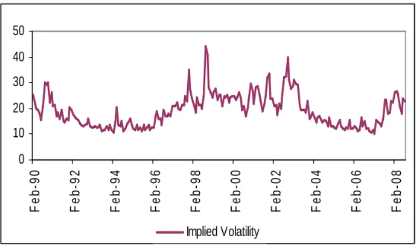
To track the implied volatility of an underlying, we need a synthetic volatility indicator. A volatility index, expressed in annualized terms, prices a portfolio of options across a wide range of strikes (volatility skew) and with constant maturity (interpolation on the volatility term structure). One widely used benchmark is the VIX. Published by the Chicago Board Options Exchange (CBOE), this index expresses the 30-day implied volatility generated from S&P 500 traded options. The details of the calculation methodology are given in a White Paper published by the CBOE in 20042. Because the

2 _{The method of calculation evolved in September 2003. The current method (applied retroactively to the index since 1990)}

takes into account S&P500 traded options at all strikes, unlike the previous VXO index, which was based solely on at-the-money S&P 100 options.

VIX reflects a consensus view of short-term volatility in the equity market, (see Figure 1), it is used to measure market participants’ risk aversion. As such, it is referred to as the "investor fear gauge".

Figure 1: Implied Volatility, February 1990 – August 2008

US Implied Volatility is represented by the VIX index

Although the VIX index itself is not a tradable product, the Chicago Futures Exchange3 launched futures contracts on it in March 2004. As a result, investors now have a simple and direct way of exposing their portfolios to variations in the short-term implied volatility of the S&P 500. VIX futures are a better way of achieving such exposure than through traditional approaches relying on delta-neutral combinations of options such as straddles, strangles or more complex strategies such as volatility-weighted combinations of calls and puts. On short maturities of less than 3 months, neutralizing the delta exposure of these portfolios can easily overshadow the impact of implied volatility variations.

To establish a structurally long investment in implied volatility, we use an approach that takes advantage of the mean-reverting nature of volatility4 (Dash and Moran (2005)). We do this by calibrating the exposure according to the absolute levels of the VIX, taking the highest exposure when

3 _{Part of the Chicago Board Options Exchange.}

4 _{Empirical tests have shown that having an exposure inversely proportional to the observed level of implied volatility}

makes the strategy much more profitable.

0 10 20 30 40 50 F e b -9 0 F e b -9 2 F e b -9 4 F e b -9 6 F e b -9 8 F e b -0 0 F e b -0 2 F e b -0 4 F e b -0 6 F e b -0 8 Implied Volatility

implied volatility is historically low, and reducing it as volatility rises. Implementing the long volatility (LV) strategy consists in buying the correct number of VIX futures such that the impact of a

1-point variation in the price of the future is equal to 1 *100%

1

−

t

F (5% impact when the level of VIX

is 20). The P&L generated between t–1 (contract date) and t (maturity date) can then be written as:

) ( 1 1 1 − − − = t t t VIX t F F F PL (1)

WhereF is the price of the future at time t. t

In practice, VIX futures prices exist only since 2004. They represent the 1-month forward market price for 30-day implied volatility. This forward-looking component is reflected in a term premium between the VIX future and the VIX index. This premium tends to be positive when volatility is low (it represents a cost of carry for the buyer of the future) and negative when it peaks. To approximate pre-2004 VIX futures prices, we used the average relationship between VIX futures and the VIX index, estimated econometrically over the period between March 2004 and August 2008 (see Figure 2 and Table 5 in Appendix 2).

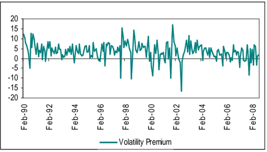
The second strategy involves taking exposure to the difference between implied and realized volatility. This difference, defined as a risk premium, has historically been positive on average for equity indices (Carr and Wu (2009)). This volatility risk premium (VRP), which is well documented in the literature (Bakshi and Kapadia (2003), Bondarenko (2006)), can be explained by the asymmetric risk between a short volatility position (a net seller of options faces an unlimited potential loss), and a long volatility position, where the loss is capped at the premium paid. To offset uncertainty on the future level of realized volatility, sellers of implied volatility demand compensation in the form of a premium over the expected realized volatility5.

5 _{Other components can provide partial explanations of this premium: the convexity of the P&L of the variance swap, and}

The VRP (see Figure 3 for a historical time series) is captured by investing in a variance swap, i.e. a swap contract on the spread between implied and realized variance. With an over-the-counter transaction, the two parties agree to exchange a specified level of implied variance for the actual amount of variance realized over a pre-agreed period. The implied variance at inception is the level that puts the net present value of the swap at zero. In theory this level (or strike) is computed from the price of the option portfolio used to calculate the volatility index itself6. The theoretical strike for a 1-month variance swap on the S&P 500 is thus the value of the VIX index. But in practice, owing to the difficulty of replicating the index, it is more realistic to reduce VIX implied volatility by 1% to reflect the replication costs borne by arbitragers (Standard & Poors (2008))7.

Figure 3: Volatility Risk Premium, February 1990 – August 2008

The Volatility Risk Premium is calculated as the difference between Implied Volatility (VIX) and Realized Volatility of the S&P500

The P&L of a short variance swap position between the start date (t–1) and end date (t) can be written as follows (Demeterfi et al. (1999)):

6 _{A variance swap can be seen as a representation of the structure of implied volatility (the volatility “smile”) since the}

strike price of the swap is determined by the prices of options with the same maturity and different strikes (all available calls/puts in, at, or out of the money) that make up a static portfolio replicating the payoff at maturity. The calculation methodology for the VIX volatility index represents the theoretical strike of a variance swap on the S&P 500 index with a maturity of one month (interpolated from the closest maturities so as to keep maturity constant).

7

From a practical standpoint, the two markets are closely linked through the hedging activity of market-makers: at a first approximation, a market-maker that sells a variance swap will typically hedge the vega risk on its residual position by buying the 95% out-of-the-money put on the listed options market.

-20 -15 -10 -5 0 5 10 15 20 F e b -9 0 F e b -9 2 F e b -9 4 F e b -9 6 F e b -9 8 F e b -0 0 F e b -0 2 F e b -0 4 F e b -0 6 F e b -0 8 Volatility Premium

[

]

Where Kt–1 is the volatility strike of the variance swap contract entered at date t–1,

100

t t

VIX

K = , VIX t

is the VIX index,RV_t−1,tis the realized volatility between t–1 and t, and N_variance is the “variance notional.”

Risk averse investors can now invest in capped variance swaps, thus fixing the maximum possible loss, or equivalently an upper limit for the realized volatility8 that will be paid. We consider a capped variance swap strategy on the S&P 500 held over a one-month period.

Stemming from equation (2) the P&L of a short capped variance swap position becomes:

[

]

variance* t (min(2.5* t , t t)) VARSWAP

t N K K RV

PL = ₋ − _{− −} (3)

In terms of the Greek-letter parameters popularized by the Black-Scholes-Merton option pricing model, the notional of a variance swap is expressed as a vega notional, representing the mean P&L of a variation of 1% (one vega) in volatility. Although the variance swap is linear in variance, it is convex in volatility since a variation in volatility has an asymmetric impact. The relationship between the two notionals is as follows:

K N

N_vega = _variance*2

Where N_vega is the vega notional of the contract.

As a consequence, equation (3) can also be rearranged as:

[

]

8 _{In practice, the standard cap is 2.5 times the strike of a variance swap (implied volatility). The investor that wants to buy}

this protection has to pay a cost that will further reduce the VIX implied volatility. In this work we consider an average cost of 0.2% (Credit Suisse (2008)).

Henceforth we refer to this way of calculating the P&L of a short variance swap, as expressed in equation (4)9.

3. PORTFOLIO CONSTRUCTION

When implementing a volatility strategy, one important aspect to take into account is the non-normality of return distributions, as shown in the next section. The mean-variance criterion of Markowitz (1952) is not suitable when returns are not normally distributed. To compensate for this, many authors have sought to include higher-order moments of the return distribution in their analysis. Lai (1991) and Chunhachinda et al. (1997), for example, introduce the third moment of the return distribution (i.e. skewness) and show that this produces significant changes in optimal portfolio construction. A further significant improvement can be achieved by extending portfolio selection to a four-moment criterion (Jondeau and Rockinger (2006, 2007)).

For investors, the main danger with the proposed volatility framework is the risk of substantial losses in extreme market scenarios (the left tail of the return distribution). Since returns on volatility strategies are not normally distributed, we choose “modified Value-at-Risk” as our reference measure of risk. Value-at-Risk (VaR) is the maximum potential loss over a time period given a specified probability α. To capture the effect of non-normal returns, we replace the quantile of the standard normal distribution with the “modified” quantile of the distributionw , approximated by the Cornish-_α

Fisher expansion based on a Taylor series approximation of the moments (Stuart, Ord and Arnold (1999)). This enables us to correct the distribution N(0,1) by taking skewness and kurtosis into account. Modified VaR is accordingly written as:

) * ( ) 1 (

α

µ

σ

9 _{We can note that with this cap the maximum loss for a short variance swap position will be equal to}

1 625 . 2 * t₋ vega K N

2 3 3 2 * ) 5 2 ( 36 1 * ) 3 ( 24 1 * ) 1 ( 6 1 S z z EK z z S z z w_α = _α + _α − + _α − _α − _α − _α

Where µand

σ

the modified percentile of the distribution at threshold

α

Modified VaR is not only easy to implement when constructing the risk budget for an investor; it explicitly takes into account how that investor’s utility function changes in the presence of non-normal returns. Modified VaR will be greater for the portfolio that has negative skewness (left-handed return distribution) and/or higher excess kurtosis (leptokurtic return distribution). A risk-averse investor will prefer a return distribution where the odd moments (expected return, skewness) are positive and the even moments (variance, kurtosis) are low.

In practice, because volatility strategies are implemented through listed or OTC derivatives, the only capital requirement is the collateral needed when entering into a variance swap contract, along with margin deposits for listed futures. Cash requirements being limited, a key step in the process of volatility investing is the proper calibration of the strategies.

Each volatility strategy is calibrated according to the maximum allowable risk exposure. Based on our computations of modified VaR for each asset class, we set monthly modified 99% VaR at 10%, a level comparable to the equity asset class (see Table 1 in the Appendix 1 ). The returns to the volatility strategies are thus the return on cash plus a fixed proportion of each strategy’s P&L. This proportion, which for simplicity we call “degree of leverage”, is determined ex ante by our calibration of the allowed risk:

VIX t f t LV t r L PL r = + ₁* (6) VARSWAP t f t VRP t r L PL r = + ₂* (7)

Where rtLV(resp. VRP t

r ) is the monthly return of the LV strategy (resp. VRP), r is the cash return,tf L1

(resp. L₂) is the degree of leverage calibrated on the LV strategy (resp. VRP).

4. DATA

Our dataset is composed of U.S. monthly figures for the period from February 1990 to August 2008. We use the 7-10 year Merrill Lynch index for government bonds, the S&P 500 for equities, the CBOE's VIX index for the volatility strategies, and the 1-month U.S. interbank rate for the risk-free rate10.

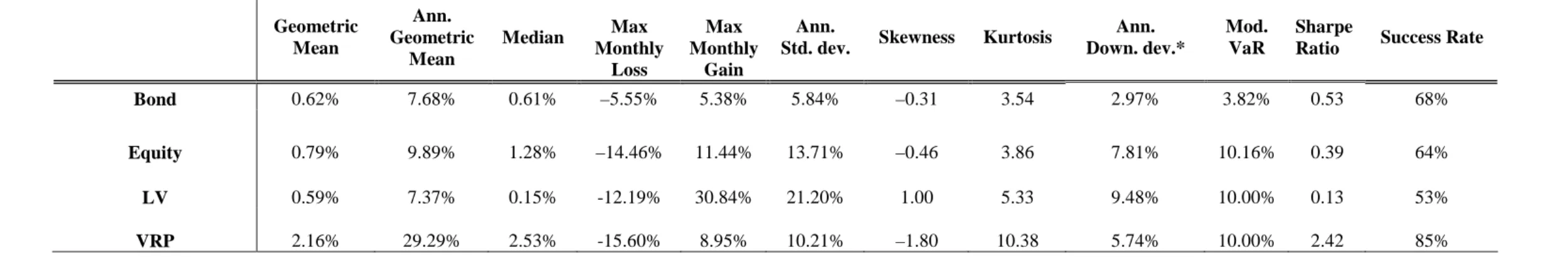
Table 1 in Appendix 1 shows the statistics for the four “assets” included in our study: government bonds, equities and the two volatility strategies. Looking at Sharpe ratios and success rates11, the VRP strategy seems to be the more attractive, with a Sharpe ratio of 2.4 and a success rate of 85%. Bonds (0.5 and 68%), equities (0.4 and 64%) and the LV strategy (0.1 and 53%) follow in that order. Although the LV strategy comes last in this ranking, it holds considerable interest in terms of diversifying power, as we will show. The VRP strategy, on the other hand, is the more consistent winner. Its performance is relatively stable, the exception being during periods of rapidly increasing realized volatility (onset of crises, unexpected market shocks), when returns are strongly negative12 and much greater in amplitude than for the traditional asset classes. These periods are usually short, accounting for only 15% of the months in the period under review.

For the chosen calibration, the LV strategy has the highest volatility (21%) followed by equities, VRP and bonds (14%, 10% and 6% respectively). Downside deviation – a measure of the

10 _{All of the data were downloaded as monthly series from Datastream.}

11 _{See Grinold & Kahn (2000) for the relation between the Sharpe ratio and the success rate.} 12

asymmetric risk on the left side of the return distribution – offers the same ranking. Monthly mean returns range between 0.59% for LV and 2.16% for VRP. An analysis of extreme returns (min and max) highlights the asymmetry of the two volatility strategies: the LV strategy offers the highest maximum return at 3.084% (its minimum return is -12.19%), whereas the VRP posts the worst monthly performance at –15.61% (with the best month at 8.95%).

The higher-order moments show clearly that returns are not normally distributed13, particularly for the two volatility strategies. This highlights the importance of taking an adequate measure of risk when optimizing the portfolio (as discussed in the previous paragraph). The skewness of equity and bond returns is slightly negative (–0.46 and –0.31 respectively), and for the VRP strategy it shows a very strong negative figure (–1.80). The only strategy showing positive skewness (1.00) is LV. Thus, being long implied volatility provides a partial hedge for the leftward asymmetry of the other asset classes. All four assets have kurtosis greater than 3: 3.54 and 3.86 for bonds and equities and even higher for the volatility strategies: 5.33 (LV) and 10.38 (VRP).

The multivariate characteristics of returns are likewise of great interest. The correlation matrices are shown in Table 2 of the Appendix 1. For the 1990–2008 period, we find good diversifying power between equities and bonds, in the form of virtually zero correlation. As expected, the LV strategy offers strong diversifying power relative to traditional asset classes. It is highly negatively correlated with equities (–61%), a phenomenon already well publicized by other studies (Daigler and Rossi (2006)). What is less well known is that the LV strategy is also weakly correlated with bonds (8%). This is an interesting and important property for a long-term conservative investor.

The VRP strategy shows quite different characteristics: it offers little diversification to equity exposure (46% correlation), but significantly more to bonds (–17%). More importantly, the two

13

For equity returns and returns on the two volatility strategies, the null hypothesis of a normality test is significantly rejected.

volatility strategies are mutually diversifying (–61% correlation). And this, as we will see, is very appealing for portfolio construction.

The importance of extreme risks means that the coskewness and cokurtosis matrices of the asset classes (Tables 3 and 414 in the Appendix 1) need to be analyzed. Positive coskewness value

skiij15 suggests that asset j has a high return when the volatility of asset i is high, i.e., j is a good hedge

against an increase in the volatility of i. This is particularly true for the LV strategy, which offers a good hedge of the VRP strategy, and to a lesser extent for equities and bonds. In contrast, the VRP strategy does not hedge the other assets efficiently because it tends to underperform when their volatility increases.

Because of positive cokurtosis value kuiiij16, the return distribution of asset i is more negatively

“skewed” when the return on asset j is lower than expected, i.e. i is a poor hedge against a decrease in the value of j. Here again we find that, unlike the VRP strategy, the LV strategy is an excellent hedge against equities – far better than a long bond. However, the two volatility strategies hedge each other quite well. Positive cokurtosis kuiijk is a sign that the covariance between j and k increases when the

volatility of asset i increases. The most interesting results are seen in periods of rising equity volatility. The LV/bonds correlation increases, whereas the VRP/bonds and VRP/LV correlations decline. Thus, during periods of equity market stress, VRP and equities both perform badly, while LV and bonds do better. Lastly, positive cokurtosis kuiijj means that volatilities of i and j tend to increase at the same

time. This is the case for all four assets. Once again, all coskewness and cokurtosis values are

14 _{We give a summary presentation of these matrices. For n= 4 assets, it suffices to calculate 20 elements for the}

coskewness matrix of dimension (4,16) and 35 elements for the cokurtosis matrix of dimension (4, 64).

15 _{The general formula for coskewness is:}

[

]

k j i k k j j i i ijk r r r E sk σ σ σ µ µ µ)( )( ) ( − − − = ,

where ri is the return on asset i and µi its mean.

16 _{The general formula for cokurtosis is:}

[

]

l k j i l l k k j j i i ijkl r r r r E ku σ σ σ σ µ µ µ µ )( )( )( ) ( − − − − =

respectively significantly different from 0 and 3, a sign that the structure of dependencies between these strategies differs significantly from a multivariate normal distribution.17

This initial analysis already highlights various advantages of the two volatility strategies within a diversified portfolio: the LV strategy delivers excellent diversification relative to equities and, to a lesser extent, bonds; the VRP strategy allows for very substantial increase in returns, at the expense of a broadly increased risk profile (extreme risks and codependencies with equities). Combining the two strategies is a particularly attractive option since they tend to hedge each others’ risks, especially in extreme market scenarios.

5. EFFICIENT PORTFOLIO WITH VOLATILITY

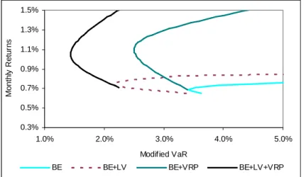
We compute efficient frontiers in a mean-VaR framework by considering a shift from a pure bond portfolio into: (1) an initial portfolio invested 100% in equities and government bonds, the initial portfolio with the addition of (2) the LV strategy, (3) the VRP strategy and (4) the two volatility strategies at the same time. As previously noted, the two volatility strategies in our analytical framework are collateralized (a fixed amount of cash is used for collateral and margin purposes). To construct the portfolio, the sum of the percentage shares in the four asset classes must equal 100%. For the two traditional asset classes (equities and bonds), the portfolio is long-only and short selling is not allowed. For the two volatility strategies implemented via derivatives, long and short positions are permitted.

Figure 4 shows the four efficient frontiers. We note firstly that adding the volatility strategies markedly improves the efficient frontier compared with the initial portfolio of equities and bonds.

Figure 4: Efficient Frontiers

Optimization results of the four Portfolios: (1) Bond Equity (BE), (2) Bond Equity + Long Volatility (BE+LV), (3) Bond Equity + Volatility Risk Premium (BE+VRP), (4) Bond Equity + Long Volatility + Volatility Risk Premium

(BE+LV+VRP), February 1990 – August 2008.

We will now examine portfolio performances that minimize VaR exposure. The corresponding allocations are presented in Table 5. Compared with the initial portfolio (76% bonds, 24% equities), the addition of the LV strategy (21%) combined with an increase in the allocation to equities (35%) and a decrease in bonds (44%) reduces the VaR to 2.1% from 3.4%. The resulting portfolio is more attractive because it has a higher Sharpe ratio (0.9 versus 0.7), obtained through higher annualized return (8.9% versus 8.3%) and lower volatility (5.0% versus 5.5%). The main reasons for this result is the strong negative correlation (–61%) between the LV strategy and equities. Furthermore, the distribution of returns for the new portfolio shows a considerable improvement in the higher-order moments. The portfolio offers positive skewness (+0.52 versus virtually nil for the initial portfolio) and an overall decrease in kurtosis from 4.12 to 3.68.

Adding the VRP strategy (30%) to the initial portfolio, at the expense of equities (0%) and, to a lesser extent, bonds (70%), delivers significantly higher returns (13.22% versus 8.28%), along with a lower VaR (2.49%). The success rate of the portfolio rises to 79.8%, and the Sharpe ratio to 1.86. The portfolio return distribution shows more pronounced leftward asymmetry (–0.41 versus +0.01), making it less attractive to the most risk-averse investors.

0.3% 0.5% 0.7% 0.9% 1.1% 1.3% 1.5% 1.0% 2.0% 3.0% 4.0% 5.0% Modified VaR M o n th ly R e tu rn s

Finally, the most interesting risk/return profile is obtained by adding a combination of the two volatility strategies. Adding both the LV (21%) and the VRP (22%), at the expense of bonds (37%) and equities (20%) makes it possible to achieve a VaR of 1.4%. The success rate increases significantly, and the Sharpe ratio (2.06) is the highest of all of the four portfolios. For a long-term investor seeking low risk exposure, the most appreciable characteristic is the decrease in extreme risks, reflected in the higher-order moments. Compared with the initial portfolio, this combined portfolio is less leptokurtic (kurtosis of 3.58 versus 4.12), and downside risk as measured by the worst-month performance is almost halved (from -3.79% to -2.03%). But the most appealing property for risk averse investors is that the portfolio exhibits positive skewness (+0.33 versus +0.01).

Table 5

Portfolio Allocation: Minimum Modified VaR U.S., February 1990 – August 2008

Summary statistics and composition of the four Minimum Modified VaR portfolios: Bond Equity, Bond Equity + Long Volatility (LV), Bond Equity + Volatility Risk Premium (VRP), Bond Equity + Long

Volatility + Volatility Risk Premium (LV+VRP). Bond Equity Bond Equity +

LV

Bond Equity + VRP

Bond Equity + LV + VRP

Mean Ann. Return 8.28% 8.94% 13.22% 12.62%

Ann. Std. Dev. 5.50% 4.98% 4.68% 3.95%

Skewness 0.01 0.52 -0.41 0.33

Kurtosis 4.12 3.68 3.41 3.58

Max Monthly Loss -3.79% -3.07% -3.23% -2.03%

Max Monthly Gain 6.20% 5.69% 4.08% 4.60%

Mod. VaR(99%) 3.41% 2.13% 2.49% 1.43% Sharpe Ratio 0.69 0.89 1.86 2.06 Success Rate 70.4% 70.4% 79.8% 84.8% Bond 76% 44% 70% 37% Equity 24% 35% 0% 20% LV - 21% - 21% VRP - - 30% 22%

For a conservative investor, typically fully invested in bonds, another way of looking at the advantage of structural exposure to volatility is to compare the portfolio characteristics with the bond asset class (first row Table 1 in Appendix 1). Comparing the Sharpe ratio and extreme risks shows that an investor fully exposed to bonds can benefit significantly by diversifying his exposure, adding

equities and LV, or even better equities, the LV and VRP strategies. These two optimal portfolios have higher Sharpe ratios and lower maximum losses than bonds. More interestingly and less obviously, they provide positive skewness (compared with a negative value for bonds and nil for the classic bond/equity exposition) without incremental kurtosis.

CONCLUSION

After several decades of analyzing portfolio choice in a mean-variance framework, investors appear to have realized the key role played by higher-order moments of return distribution. Examples of how extreme risk can rise due to systematic efforts to minimize volatility are now well documented, and investors are aware of them, sometimes to their cost. In this context, a long-term investor will pay close attention to all the codependencies between asset classes in his current portfolio and to the way they change when new classes are added. A suitable strategic allocation will attempt to deliver the required long-run returns while decreasing volatility and kurtosis and increasing skewness (i.e. reducing leftward asymmetry and even obtaining rightward asymmetry).

This analysis highlights that when viewed as an asset class, volatility is an extremely attractive tool for long-term investors. Recent literature has begun to show the merits of including long exposure to implied volatility in a pure equity portfolio (Daigler and Ross (2006)) or in a portfolio of funds of hedge funds (Dash and Moran (2006)). Our study underscores the new possibilities available to long-term investors in long-terms of portfolio choice when volatility is introduced into a portfolio of classic assets (equity and bonds). Little has been written on this subject so far.

The results of our a historical analysis of the past twenty years show that including these volatility strategies in a portfolio is highly appealing. Taken separately each strategy displaces the efficient frontier significantly outward, but combining them produces even better results. Long-exposure to volatility is particularly valuable for diversifying a portfolio with equities. Because this

strategy is negatively correlated with the asset class, its hedging function during bear-market periods is clearly attractive. A volatility risk premium strategy, on the other hand, boosts returns. It provides little diversification to equities – it loses significantly when share prices fall – but good diversification with respect to bonds and implied volatility. Combining the two strategies offers the big advantage of fairly effective reciprocal hedging during periods of market stress, which significantly improves portfolio returns for a given level of risk.

One of the limitations of our work relates to the period analyzed. Although markets experienced several severe crises between 1990 and 2008, with sharp volatility spikes, there is no assurance that future crises will not be more acute than those experienced over the testing period or that losses on variance swap positions will not be greater, thereby partly erasing the high reward associated with the volatility risk premium. One interesting continuation of this work would be to explore the extent to which long exposure to volatility is a satisfactory hedge of the volatility risk premium strategy during periods of stress and sharply rising realized volatility. In any case, an essential aspect of using volatility as an asset class is the significant possibilities it offers for tailoring a portfolio to an investor's needs, especially if he is risk averse. Over the long term, volatility strategies make it possible to build portfolios that are more efficient than a pure-bond or equity/bonds investment, within a framework that goes beyond simple mean-variance.

REFERENCES

Agarwal V. and Naik N. (2004), “Risks and Portfolio Decisions Involving Hedge Funds”, Review of Financial Studies, 17(1), p. 63–8.

Allen P., Einchcomb S. and Granger N. (2006), “Variance Swaps”, JP Morgan European Equity Derivatives Strategy, 14 November.

Amenc N., Goltz F. and Martellini L. (2005), “Hedge Funds from the Institutional Investor’s Perspective”, in Hedge Funds: Insights in Performance Measurement, Risk Analysis, and Portfolio Allocation, edited by Gregoriou G., Papageorgiou N., Hubner G. and Rouah F., John Wiley.

Amin G. and Kat H. (2003), “Stocks, Bonds and Hedge Funds: Not a Free Lunch!”, Journal of Portfolio Management, 29 (4), p. 113-120.

Bakshi G. and Kapadia N. (2003), “Delta-Hedged Gains and the Negative Market Volatility Risk Premium”, The Review of Financial Studies, 16 (2), p. 527–566.

Bekaert G. and Wu G. (2000), “Asymmetric Volatilities and Risk in Equity Markets”, Review of Financial Studies, 13(1), p. 1-42.

Black F. (1976), “Studies in Stock Price Volatility Changes”, Proceedings of the 1976 Business Meeting of the Business and Economic Statistics Section, American Statistical Association, p. 177-181.

Bollen N.P.B. and Whaley R.E. (2004), “Does Net Buying Pressure Affect the Shape of Implied Volatility Functions”, The Journal of Finance, 59(2), p. 711–753.

Bondarenko O. (2006), “Market Price of Variance Risk and Performance and Hedge Funds”, AFA 2006 Boston Meetings Paper.

Carr P. and Madan D. (2001), “Optimal Positioning in Derivative Securities”, Quantitative Finance, 1(1), p. 19-37.

Carr P. and Wu L. (2009), “Variance Risk Premiums”, Review of Financial Studies, 22(3), p. 1311-1341.

CBOE (2004), “VIX CBOE Volatility Index”, Chicago Board Options Exchange Web site.

Chunhachinda P., Dandapani K., Hamid S. and Prakash A.J. (1997), “Portfolio Selection With Skewness: Evidence from International Stock Markets”, Journal of Banking and Finance, 21(2), p. 143– 167.

Christie A.A. (1982), “The Stochastic Behavior of Common Stock Variances:Value, Leverage and Interest Rate Effects”, Journal of Financial Economics, 10, p. 407-432.

Credit Suisse (2008), “Credit Suisse Global Carry Selector”, October.

Daigler R.T. and Rossi L. (2006), “A Portfolio of Stocks and Volatility”, The Journal of Investing, 15(2), Summer, p. 99-106.

Dash S. and Moran M.T. (2005), “VIX as a Companion for Hedge Fund Portfolios”, The Journal of Alternative Investments, 8(3), Winter, p. 75-80.

Demeterfi K., Derman E., Kamal M. and Zhou J. (1999), “A Guide to Volatility and Variance Swaps” The Journal of Derivatives, 6(4), Summer, p. 9-32.

Egloff D., Leippold M. and Wu L. (2007), “Variance Risk Dynamics, Variance Risk Premia and Optimal Variance Swap Investments”, EFA 2006 Zurich Meetings Paper, SSRN eLibrary,

http://ssrn.com/paper=903728.

Favre L. and Galeano J.A. (2002), “Mean-modified Value at Risk Optimization With Hedge Funds”, Journal of Alternative Investment, 5(2), Fall, p. 21-25.

French K.R., Schwert G.W. and Stambaugh R.F. (1987), “Expected Stock Return and Volatility”, Journal of Financial Economics, 19, p. 3-30.

Glosten L.R., Jangannathan R. and Runkle D.E. (1993), “On the Relation Between Expected Value and the Volatility of the Nominal Excess Return of Stocks”, Journal of Finance, 48(5), p. 1779-1801.

Guidolin M. and Timmerman A. (2005), “Optimal Portfolio Choice under Regime

Switching, Skew and Kurtosis Preferences”, Working Paper, Federal Reserve Bank of St. Louis.

Hafner R. and Wallmeier M. (2008), “Optimal Investments in Volatility”, Financial Markets and Portfolio Management, 22(2), p. 147-167.

Harvey C., J. Liechty, M. Liechty and P. Müller (2003), “Portfolio Selection with Higher Moments”, Working Paper, Duke University.

Haugen R.A., Talmor E. and Torous W.N. (1991), “The Effect of Volatility Changes on the Level of Stock Prices and Subsequent Expected Returns”, Journal of Finance, 46 (3), p. 985-1007.

Jondeau E. and M. Rockinger (2006), “Optimal Portfolio Allocation under Higher Moments”, Journal of the European Financial Management Association 12, p. 29–55.

Jondeau E. and M. Rockinger (2007), “The Economic Value of Distributional Timing”, Swiss Finance Institute Research Paper 35.

Kim C.J., Morley J., Nelson C. (2004), “Is there a Positive Relationship between Stock Market Volatility and the Equity Premium?”, Journal of Money, Credit, and Banking, 36(3), p. 339-360.

Kotz S., Balakrishnan N. and Johnson N.L. (2000), “Continuous Multivariate Distributions, Volume 1: Models and Applications”, John Wiley, New York.

Kuenzi D.E. (2007), “Shedding Light on Alternative Beta: a Volatility and Fixed Income Asset Class Comparison”, Volatility as an Asset Class, Israel Nelken ed., London: Risk Books.

Lai T.Y. (1991), “Portfolio Selection with Skewness: A Multiple Objective Approach”, Review of Quantitative Finance and Accounting, 1, p. 293–305.

Liu J. and Pan J. (2003), “Dynamic Derivative Strategies”, Journal of Financial Economics, 69, p. 401-430.

Markowitz H., (1952), “Portfolio Selection”, Journal of Finance 7(1), p. 77–91.

Martellini L. and Ziemann V. (2007), “Extending Black-Litterman Analysis Beyond the Mean-Variance Framework”, Journal of Portfolio Management, 33(4), Summer, p. 33-44.

Schwert G.W. (1989), “Why Does Stock Market Volatility Change over Time?”, Journal of Finance, 44 (5), p. 1115-1153.

Sornette D., Andersen J.V. and Simonetti P. (2000), “Portfolio Theory for Fat Tails”, International Journal of Theoretical and Applied Finance, 3(3), p. 523–535.

Standard & Poors (2008), “S&P500 Volatility Arbitrage Index: Index Methodology”, January.

Stuart A., Ord K. and Arnold S.(1999), “Kendall’s Advanced Theory of Statistics, Volume 1 : Distribution Theory”, 6th edition, Oxford University Press.

Turner C.M., Starz R. and Nelson C.R. (1989), “A Markov Model of Heteroskedasticity, Risk and Learning in the Stock Market”, Journal of Financial Economics, 25, p. 3-22.

Wu G. (2001), “The Determinants of Asymmetric Volatility”, Review of Financial Studies, 14, p. 837-859.

Appendix 1 : Descriptive Statistics

Table 1 Descriptive Statistics US, February 1990 – August 2008

Summary statistics of monthly returns of Bonds, Equities, Long Volatility (LV) and Volatility Risk Premium (VRP).

*Downside Deviation is determined as the sum of squared distances between the returns and the cash return series. Geometric Mean Ann. Geometric Mean Median Max Monthly Loss Max Monthly Gain Ann.

Std. dev. Skewness Kurtosis

Ann. Down. dev.*

Mod. VaR

Sharpe

Ratio Success Rate Bond 0.62% 7.68% 0.61% –5.55% 5.38% 5.84% –0.31 3.54 2.97% 3.82% 0.53 68%

Equity 0.79% 9.89% 1.28% –14.46% 11.44% 13.71% –0.46 3.86 7.81% 10.16% 0.39 64%

LV 0.59% 7.37% 0.15% -12.19% 30.84% 21.20% 1.00 5.33 9.48% 10.00% 0.13 53%

Table 2

Correlation matrix, US, February 1990–August 2008

Correlation matrix of monthly returns of Bonds, Equities, Long Volatility and Volatility risk premium.

Bonds Equity LV VRP Bonds Equity –0.01 LV 0.08 –0.61 VRP –0.17 0.46 –0.60 Table 3 Co-Skewness matrix US, February 1990 – August 2008

Co-skewness matrix of monthly returns of Bonds, Equities, Long Volatility and Volatility Risk Premium. Bonds^2 Equity ^2 LV^2 VRP^2 Bonds*Equity Bonds*LV Equity*LV Bonds –0.31 0.35 0.05 0.47 Equity –0.03 –0.46 –0.67 –0.84 LV 0.21 0.59 1.00 0.89 –0.13 VRP –0.15 –0.50 –0.71 –1.80 0.22 –0.21 0.57 Table 4 Co-kurtosis matrix US, February 1990 – August 2008

Co-kurtosis matrix of monthly returns of Bonds, Equities, Long Volatility and Volatility Risk Premium.

Bonds^3 Equity ^3 LV^3 VRP^3 Bonds* Equity^2 Bonds* LV^2 Bonds* VRP^2 Bonds 3.54 –0.53 0.98 –2.49 1.53 1.39 1.34 Equity 0.26 3.86 –3.57 4.57 –0.53 –0.84 –1.24 LV 0.15 –2.81 5.33 –4.75 0.76 VRP –0.42 2.13 –3.79 10.38 –0.81 –1.04 Equity* LV^2 Equity* VRP^2 Bond^2* Equity Bond^2* LV Equity^2* VRP LV^2* VRP Equity*LV* VRP Bonds 0.86 Equity 3.04 2.99 LV –2.85 –0.97 –2.30 VRP 2.75 0.69 –0.91 3.66

Appendix 2 : VIX future estimation

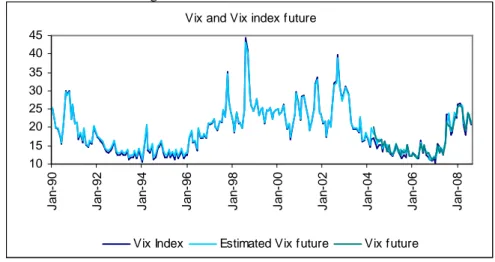
Figure 2: VIX Index, VIX Index future and estimation, February 1990 – August 2008

The VIX Index future is represented by the 1 month contract, VIX future estimation is realized trough a linear regression between VIX and VIX Index.

Table 5

VIX Index and VIX Index future estimate

Results of the regression of the 1 month VIX Index future on the VIX Index, March 2004 - August 2008.

α represents the constant, β the slope coefficient, the last three columns report the adjusted R squared, the Standard Errorof the regression and the Durbin Watson statistic.Standard errors in parenthesis.

α (t stat) β (t stat) Adjusted R2 SE of regression DW test

1.30 0.95 0.95 0.94 1.54

VIX future

(2.74) (32.67)

Vix and Vix index future

10 15 20 25 30 35 40 45 J a n -9 0 J a n -9 2 J a n -9 4 J a n -9 6 J a n -9 8 J a n -0 0 J a n -0 2 J a n -0 4 J a n -0 6 J a n -0 8