HAL Id: hal-01239705
https://hal.archives-ouvertes.fr/hal-01239705
Submitted on 30 Jun 2016
HAL is a multi-disciplinary open access
archive for the deposit and dissemination of
sci-entific research documents, whether they are
pub-lished or not. The documents may come from
teaching and research institutions in France or
L’archive ouverte pluridisciplinaire HAL, est
destinée au dépôt et à la diffusion de documents
scientifiques de niveau recherche, publiés ou non,
émanant des établissements d’enseignement et de
recherche français ou étrangers, des laboratoires
Array Size Computation under Uniform Overlapping
and Irregular Accesses
Angeliki Kritikakou, Francky Catthoor, Vasilios Kelefouras, Costas Goutis
To cite this version:
Angeliki Kritikakou, Francky Catthoor, Vasilios Kelefouras, Costas Goutis. Array Size Computation
under Uniform Overlapping and Irregular Accesses. ACM Transactions on Design Automation of
Electronic Systems, Association for Computing Machinery, 2016, 21, pp.1-35. �10.1145/2818643�.
�hal-01239705�
Array Size Computation under Uniform Overlapping & Irregular
Accesses
ANGELIKI KRITIKAKOU, IRISA & Dep. Computer Science & Electrical Engineering, Univ. of Rennes 1
FRANCKY CATTHOOR, IMEC & Dep. Electrical Engineering, Kath.Univ. Leuven VASILIOS KELEFOURAS, Dep. Electrical & Computer Engineering, Univ. of Patras and COSTAS GOUTIS, Dep. Electrical & Computer Engineering Univ. of Patras
The size required to store an array is crucial for an embedded system, as it affects the memory size, the energy per memory access and the overall system cost. Existing techniques for finding the minimum number of resources required to store an array are less efficient for codes with large loops and not regularly occurring memory accesses. They have to approximate the accessed parts of the array leading to overestimation of the required resources. Otherwise their exploration time is increased with an increase over the number of the different accessed parts of the array. We propose a methodology to compute the minimum resources required for storing an array which keeps the exploration time low and provides a near-optimal result for regularly and non-regularly occurring memory accesses and overlapping writes and reads.
Categories and Subject Descriptors: B.3.2 [Memory structures]: Design Styles—Primary Memory; C.3 [Special purpose and Application-Based Systems]: Real-time and Embedded Systems; D.3.4
[Pro-gramming Languages]: Processors—Compilers, Optimization; E.1 [Data Structures]: Arrays
General Terms: Design
Additional Key Words and Phrases: Liveness, Resources Optimization, Near-optimality, Scalability, Itera-tion Space
1. INTRODUCTION
The size required to store the information in a system is crucial for several domains, because it is directly coupled with the cost of the system, the required area and the energy consumption [Catthoor 1999]. Such examples are the scratchpad memories of embedded systems [Gr¨osslinger 2009], the hardware controlled caches of general pur-pose systems [Catthoor 1999] and the industry storage management systems, such as cargo [Lee et al. 2007]. In the embedded systems the memories have an important part in the overall system cost [Catthoor 1999]. The embedded applications, such as image, video and signal processing, mostly use arrays as data structures. Then, the size required to store the arrays becomes an essential part of the overall system de-sign cost. An overestimated size leads to increase in the memory size, the chip area and the system energy consumption.
In this work we are computing the minimum size required to store an array un-der a given schedule, which is required in memory optimizations and more
pre-Author’s address: A. Kritikakou, Dep. Computer Science & Electrical Engineering, Univ. of Rennes 1, & IRISA-INRIA 35000, Rennes, France, angeliki.kritikakou@irisa.fr, C. Goutis, V. Kelefouras: Univ. of Patras, Dep. Electrical & Computer Engineering, Rio, Patras, Greece, 26500, F. Catthoor: Inter-university Micro-Electronics Center, Kapeldreef 75, 3001 Leuven, Belgium
Permission to make digital or hard copies of part or all of this work for personal or classroom use is granted without fee provided that copies are not made or distributed for profit or commercial advantage and that copies show this notice on the first page or initial screen of a display along with the full citation. Copyrights for components of this work owned by others than ACM must be honored. Abstracting with credit is per-mitted. To copy otherwise, to republish, to post on servers, to redistribute to lists, or to use any component of this work in other works requires prior specific permission and/or a fee. Permissions may be requested from Publications Dept., ACM, Inc., 2 Penn Plaza, Suite 701, New York, NY 10121-0701 USA, fax +1 (212) 869-0481, or permissions@acm.org.
c
YYYY ACM 1539-9087/YYYY/01-ARTA $15.00 DOI:http://dx.doi.org/10.1145/0000000.0000000
cisely in the intra-signal in-place step of the Data Transfer and Storage Exploration (DTSE) [Catthoor et al. 1998]. The size is defined by the maximum number of array el-ements that are concurrently alive, i.e. all the elel-ements that have been already stored (written) in memory and they will be loaded (read) in the future. When the writes and the reads to the array are overlapping, the complexity of the computation of the max-imum number of alive elements is increased. In the overlapping case the reads of the array start before all the writes have finished. Therefore, the number of concurrently alive elements is not unique among iterations, as the lifetime of each element can be different. The overlapping case is different from the non-overlapping one [Kritikakou et al. 2013]. In the latter, all the reads to the array are performed after all the writes have finished and thus the maximum number of concurrently alive elements is the footprint of the array.
Existing techniques to compute the minimum size required to store an array are enumerative, symbolic/polyhedral or approximations, as described in Section 10. The enumerative approaches find the optimal size, i.e. the exact number of concurrently alive elements. However, when the array size is increased, the required exploration time to find the size is highly increased. The symbolic/polyhedral approaches [De Greef et al. 1997; Cohen et al. 1999; Darte et al. 2005; Clauss et al. 2011] use inequalities to describe the edges of the shapes that describe the accessed parts of the array. They provide the maximum number of alive elements by finding the maximum number of integers through an ILP solver. Hence, when the array size is increased, some values in the inequalities are modified, and thus, they are scaling well providing exact results. However, when the accesses to the array are not regularly occurring, i.e. they become irregular, the shape that describes an accessed part of the array loses its solidity, i.e. regions exist inside the shape which are not accessed, creating holes. In addition, the number of shapes of the accessed parts are increased and these shapes may not be regularly repeated in the space. This irregularity is created by the data dependent and the use case dependent array accesses. When the shapes of the accessed parts are not similar to polyhedra or lattices, the symbolic/polyhedral approaches lose their ability to efficiently describe them. The number of inequalities required to describe the edges of the accessed shapes is increased, increasing the time of the ILP solver. To reduce the number of inequalities and thus the exploration time, the shapes can be approxi-mated, for instance using (approximated) convex hulls or approximated enumerators. However, no control exist over the quality of the approximation. An approximated con-vex hull can be applied to solidify both the holes inside and between the accessed parts in order to create a simple shape. However, this process can highly overestimate the number of concurrently alive elements leading to an overestimation of the size of the required resources.
The notation used in the rest of this paper is summarized in Table I. The paper organization is: Section 2 describes the motivation of our work providing relevant ex-amples, Section 3 describes the contribution of the proposed methodology. Section 4 describes the target domain and the input to our approach, Section 5 described the translation of the access scheme into patterns and Section 6 describes the computation of the size. Section 7 and 8 presents the closed form solutions for several cases. Sec-tion 9 presents evaluaSec-tion results. SecSec-tion 10 presents the related work on techniques using the maximum number of concurrently alive elements. Section 11 concludes this study.
2. MOTIVATION
The high irregularity in the array accesses of the applications derives from aspects that cannot be modelled accurately statically and from different operation modes or
Table I: Summarized notation of the proposed methodology.
SIS Solid Iteration Space
ISH Iteration Space with Holes
ECS Enumerative Conditions for SIS
ECH Enumerative Conditions for ISH
PCS Parametric Conditions for SIS
PCH Parametric Conditions for ISH
SIR Segment Iterator Range
ST Segment Type
LB Lower Bound
UB Upper Bound
IR Iterator Range of pattern (IR=UB-LB-1)
PS Pattern Size (P S =PN
i=0SIR(i))
RF Repetition factor (RF = IR
P S)
N Total number of pattern segments
Diff Exploration window, i.e. index difference of RD and WR
SID(i) Segment Iterator Domain of i pattern segment
HID(i) Hole Iterator Domain of i pattern segment
Sizei Size of i dimension
PSizei Partial size of exploration window of i dimension Asizei Additional elements of exploration window of i dimension
CP Combined Pattern
ADiff Maximum number of A in the pattern section
HDiff Maximum number of H in the pattern section
extraPCH= Additional elements due to a PCH of == type
extraPCH=,A2A Additional elements due to combination of PCHs of == type extraPCH6= Additional elements due to PCH of6= type
extraWR Computation of additional written elements
extraRD,A Computation of additional not yet read elements before the exploration window where the WR state-ment is A
extraRD,H Computation of additional not yet read elements before the exploration window where the WR state-ment is H
use cases of the application. For instance, different video decoder modes like I, P and B frames with different submodes [Juurlink et al. 2012] and applications with data dependent conditions and loop bounds.
To deal with the different use cases or to remove the data dependencies in order to continue with an efficient Design Space Exploration (DSE), the system scenarios ap-proach [Filippopoulos et al. 2014; Filippopoulos et al. 2012; V.Gheorghita et al. 2009] is a very promising direction. The alternative of considering the general worst case of all the modes and the code instances leads to pessimistic over-approximations. The sys-tem scenarios approach explores the potential values of the data and their effect in the application. Based on this information it groups similar instances of the application code into a common scenario. Due to the initial data dependencies the resulting appli-cation instances have highly irregular array accesses. Now, we can use the worst case code instance per scenario to continue with the DSE. The result of the system scenario approach is a number of scenarios that have to be explored, where each scenario has a different code instance with irregular array accesses. The number of code instances to be explored is equal to the number of scenarios. A trade-off exists between the num-ber of scenarios and the similarity in the code instances. In this paper we do not deal with the system scenario creation, but we use the resulting codes as an input to our methodology. More information about the memory-aware system scenario approaches is presented in [Filippopoulos et al. 2014].
As we now have to explore a number of different application instances in this DSE step, a general parametric approach is not applicable. The time required to explore one instance becomes now an important factor in the overall time of DSE, as we need to apply this step a lot of times in order to explore a set of different scenarios for the application under study and we have to apply this process for all the arrays existing in the application. To provide an intuition over the gains in the overall flow, we will use
the information provided in [Balasa et al. 2008] using the STOREQ, a tool developed for main parts of the steps [Kjeldsberg et al. 2003]. This tool is typically used in the inner core of a loop transformation exploration kernel. The number of different loop organisation schemes that have to be explored can be huge, e.g. for permutations it is exponential and by adding loop splits this number is prohibitively increased. For instance, for the Darwin algorithm with 27 arrays we observe the longest time for the overall flow, i.e. 2.5s [Balasa et al. 2008]. Assuming that the array size computation for polyhedral approach takes 81 ms, which was the lower value obtained during our experimentations, then the total time dedicated to the computation of the maximum alive elements for all the arrays is 2.187s, which is the dominant task as it takes 88% of the total time. Replacing this step with the proposed approach (which in the worst observed case takes 0.902 ms), we need 24.36ms for this step (a gain factor of 89.77) and the total time is 337.36ms (gain factor of 7.4). As the computation of the maximum number of alive elements is one step in the overall DSE process, we should keep the exploration time reasonable, while providing a near-optimal result.
The near-optimality of this DSE step is essential, as the obtained result is used in the next memory DSE phases, i.e. inter-signal in-place optimization, memory access scheduling and memory address generation [Catthoor 1999], and thus the quality of the result of this step affects the quality of the next phases. Therefore, we do not want to increase the memory size without a reason.
As a high level of irregularity exists in the array accesses inside each code in-stance, the existing approaches either require a higher exploration time to find an near-optimal solution or they have to approximate the result. The enumerative ap-proaches add the writes between the iteration where an element is written and the iteration where this element is read for the last time. This process is repeated for all the elements of the array. Hence, when the number of the accesses is increased, they require significant exploration time. The symbolic/polyhedral approaches can repre-sent the irregular space as unions of polytopes. However, when the number of dif-ferent polytopes is increased, the exploration time is also increased. The alternative is to approximate the array accesses by applying (approximated) convex hulls which can over-approximate the size as the approximation is not performed in a controlled way. The proposed methodology remains scalable and near-optimal, as it represents the array accesses as patterns with accesses and holes and it combines iteratively the patterns to find the required size. In case long patterns occur, the knowledge of the holes allows us to approximate in a controlled way. By selecting few small holes to be considered as accesses, the size of the patterns and the time of the proposed approach are reduced. More details are provided in the rest of the manuscript.
2.1. Examples
Real-life applications are characterized by dynamic behavior which is also reflected in fluctuating memory requirements [Filippopoulos et al. 2014]. Then, the conventional allocation and assignment of data remains suboptimal. One example of such a code is Hough transformation [Duda and Hart 1972], where the element of the accumulator array that is accessed each time depends on the value of the image pixel and its po-sition. Therefore, the accesses to the accumulator array are highly irregular without following any specific pattern. In a conventional assignment the memory size used for the storage of the accumulator is determined by the dimensions of the input image us-ing the worst-case area for the accumulator array variable. However, only a part of the allocated space may be accessed. To improve the memory management, memory-aware system scenario approaches are applied [Filippopoulos et al. 2014], which create a set of scenarios with different code instances describing highly irregular accesses to the accumulator.
For (i=0; i<14; i++) For (j=0; j<7; j++) If ((i>4j)&&(i<4j+3)||(i==2j+1)) If (i<12)&&(j<6) B[i][j]=... If (i>1)&&(j>0) ...=B[i-2][j-1] (a) Overlapping
For (i=0; i<12; i++) For (j=0; j<6; j++)
If ((i>4j)&&(i<4j+3)||(i==2j+1)) B[i][j]=...
For (i=2; i<14; i++) For (j=1; j<7; j++) If (i>4j-2)&&(i<4j+1)||(i==2j+1) ...=B[i-2][j-1] (b) Non-overlapping J I C1 (c) J I C2 (d) J I WR: B[I][J] (e) J I RD: B[I-2][J-1] (f)
For (i=0; i<21; i++) For (j=0; j<6; j++)
If (j==0)||(j==3)||(j==4)) ||
((i<2) || (i>3)&&(i<7) || (i==8) || (i>9)&&(i<12)) B[i][j]=...
If (j==0)||(j==3)||(j==4)) ||
((i>10)&&(i<13) || (i>14)&&(i<18) || (i==19) || (i<20)) ...=B[i-11][j] (g) Enumerative overlapping I J WRITE READ 0 (h) I J WRITE READ I WRITE READ I WRITE READ I WRITE READ I WRITE READ I WRITE READ K 0 (i)
Fig. 1: Application code for (a) overlapping and (b) non-overlapping case, iteration spaces where the boxes describe accesses of the (c) C1, (d) C2, (e) written elements, (f) read elements, (g) overlapping application code with enumerative conditions, (h) iteration space with accesses and (i) extension to 3 dimensional case.
In the examples of the paper we keep the iteration space small for demonstration reasons. Fig. 1 explores how the existing approaches behave on the different code in-stances with high irregularity derived from the memory-aware scenario. The overlap-ping application code is depicted in Fig. 1(a) and the non-overlapoverlap-ping code in Fig. 1(b) to illustrate the difference between these two cases. The non-overlapping code consists of two nested loops. The first loop performs aWRstatement B[i][j] with conditions C1: (i > 4j)&&(i < 4j + 3) and C2: i == 2j + 1 combined with an OR operation. The second loop performs aRDstatement B[i-2][j-1] with conditions C1: (i > 4j − 2)&&(i < 4j + 1) and C2: i == 2j + 1 combined with an OR operation. The index difference of the RD
and theWRstatement is 2 in I dimension and 1 in J dimension. The overlapping code consists of one nested loop with the same conditions and some additional ones which describe the beginning and the end of the iteration space of the WR and RD state-ments. In the overlapping case at least in one iteration theWRand theRDstatements are both executed. For instance, we observe that when I=3 and J=1 both aWR and a
RDoccurs to array B. The element B[1][0] is read and the element B[3][1] is written, as depicted by the corresponding box in the iteration I=3 and J=1 at Fig.1(e) and Fig.1(f). For this iteration, the number of alive elements is 2. For a later iteration (I=6, J=1), the element B[6][1] is written, but no read occurs to free a memory position increasing the number of alive elements to 3. In contrast, in the non-overlapping case during the iterations where the writes are executed, no read occurs at the array. Therefore, by ap-plying the solutions of the non-overlapping case [Kritikakou et al. 2013], the number of alive elements will be computed equal to 11.
When only one of the conditions C1 or C2 exists, the access shape consists of holes repeated in a regular way (Fig. 1(c) and Fig. 1(d)). This regular access scheme is ef-ficiently represented by the symbolic/polyhedral approaches [Franssen et al. 1993; Darte et al. 2005; Clauss et al. 2011]. When both conditions coexist, the repetition of the first access shape C1 is disturbed due to the second access shape C2. In this ex-ample, the symbolic/polyhedral approaches represent the space as the union between these two polytopes. For the example of Fig. 1(a), the exploration time is 627 ms for the polyhedral approach [Verdoolaege et al. 2013] and 27.8 sec for the enumerative approach to find the optimal result. However, when the number of different polytopes is increased, the exploration time is also increased, as shown in the experimental re-sults. Another example is provided in Fig. 1(h) (code of 1(g)) which depicts the access shape of aWRfor a two dimensional case. The symbolic/polyhedral approaches need at least 6 polytopes to describe the access shape when intersection and union are used in the representation and 3 when subtraction is also included. The more irregularity is present, the more polytopes are required to describe the space. The exploration time is 862 ms for the polyhedral approach and 38.8 sec for the enumerative approach to find the optimal result. The alternative is to approximate the accessed region by a convex hull. In this example, the holes of size 2x2 and 1x2 are considered as accesses and the computed size is 55, instead of 47, and thus a loss of 17% is observed. By adding an-other dimension, as depicted in Fig.1(i), the loss due to the convex hull approximation, which is 8 in our example, is increased, as it is multiplied by the size of the dimension K. The exploration time is 1482 ms for the polyhedral approach and 1223.5 sec for the enumerative approach.
2.2. Target domain & Problem formulation
The domain under study consists of applications of one thread with high memory activ-ity and with and without varying memory access intensactiv-ity [Filippopoulos et al. 2014], which possibly depends on input data variables. Such examples are high-speed data intensive applications in the fields of speech, image and video processing, which re-quire significant amount of storage resources [Jha et al. 1997]. In the case of varying memory activity, a static study of the application code is insufficient since the appli-cations have non-deterministic behaviour and thus memory-aware systems scenario approaches are applied to remove the dynamic behavior by creating a number of sce-narios [Filippopoulos et al. 2014]. Each scenario has different code instances with de-terministic behaviour and high irregularity.
Therefore, the proposed methodology is applied to applications that have static con-trol flow and regular and irregular array accesses. The irregularity derives from ap-plications with data dependent accesses to the arrays through non-manifest condi-tions and non statically known loop bounds. Applicacondi-tions with static nested loops and manifest conditions, i.e. they can be analyzed to deduce which values they take with-out executing the program, can also destroy the regularity of array accesses but in a lower degree than the data dependent accesses. After applying the system scenario approach [Filippopoulos et al. 2014; V.Gheorghita et al. 2009], we obtain a set of codes instances of the initial application with static nested loops and manifest affine
condi-tions, which describe different and irregular accesses to the arrays. Then, the worst case code instance is explored to find the minimum required size to store the arrays. However, in this work we deal with the computation of the maximum number of alive elements, whereas the creation of systems scenarios is described in [Filippopoulos et al. 2014].
Our approach focuses on the computation of the size of an array, which belongs to the intra-signal in-place optimization step of the DTSE. The DTSE methodology [Catthoor et al. 1998] has three phases: (1) the pruning phase which preprocesses the program to enable the optimization phase, (2) the DTSE methodology that optimizes the prepro-cessed program and derives a memory hierarchy and layout, and (3) the depruning and address optimization to remove the overhead introduced by DTSE. During the pruning phase the Dynamic Single Assignment (DSA) form is used to represent the applications in order to enable the memory optimizations. Several techniques exist to write the ap-plication in DSA form, such as the work in [Feautrier 1988; Vanbroekhoven et al. 2003; Vanbroekhoven et al. 2005]. The code application for our methodology writes at most once each array element during the execution of the program, but it can read it several times [Vanbroekhoven et al. 2005]. An example of transforming to DSA form is the DGEMM of two two-dimensional arrays, where C[N][N] becomes C[N][N][N] and the 3rd dimension is used to index the values produced by the k loop. When we consider the complete application and array C is used later by another part of the program, then the number of maximum alive elements we compute using our methodology is N2. Potential storage overhead introduced by the DSA due to the elimination of the
write-after-write dependencies can be removed as the in-place mapping intentionally destroys the DSA property [Vanbroekhoven et al. 2007]. The result of our methodol-ogy provides the minimal array size for the DSA. The values of the array elements that are no longer needed can be overwritten by changing the indexation of the assign-ments [Eddy De Greef and de Man 1996; Tronon et al. 2002].
After the memory management is completed by DTSE, all the required in-formation is available to execute the address optimization and the final map-ping/allocation [Catthoor et al. 1998]. The proposed approach supports an efficient address scheme achieved when the addresses are quite regular, as it does not allow exhaustive enumeration of accesses and uses repetitive patterns. When the size of patterns is increased, the proposed methodology provides a control to reduce it by con-sidering holes in the accesses with low repetition factor and of small size as virtual accesses. In this way, the address complexity is reduced.
3. CONTRIBUTION
The contribution of this work is to propose a methodology which computes the max-imum number of concurrently alive array elements keeping the exploration time low and providing a controlled approximation when required, resulting to a near-optimal and scalable approach. Compared to existing approaches, the proposed methodology achieves low exploration time and near-optimal results in complex iteration spaces with both regular and irregular array accesses and overlapping writes and reads, as also verified by the experimental results in the Section 9.
The proposed methodology consists of three steps as depicted in Fig.2: the analysis, the translation and the computation. When the methodology is applied, the steps are executed following a sequence and the information is propagated from the analysis to the computation step.
The analysis extracts the access scheme from the application code. As described in Section 4, the input code is described by a parametric template. By parsing the code under study, the template is instantiated. In this way we extract the access scheme, which is propagated to the translation step.
Analysis Translation Computation
C1 C2 C3 C4
For (I>LBI; I<UBI; I++)
For (J>LBJ; J<UBJ; I++)
... If (CI)... ...=Fx(B[I+bI]...) 1Segment N Segment Pattern I: Pattern J: . .
. Cases & Solutions
Application Patterns 1Segment N Segment Access scheme extracted from application code Dimension pattern sequences
Fig. 2: Methodology steps.
The translation step stores the access scheme received by the analysis step in a near-optimal and scalable way using the representation of the pattern formulation presented in [Kritikakou et al. 2014]. The patterns and the pattern operations are applied per dimension. A pattern is a sequence of segments that describe Accesses (A) or Holes (H), i.e. not accesses, to the array and has a set of parameters that describe the position and the repetition of the pattern in the iteration space. In case more than one pattern refers to the same parts of the iteration space, pattern operations are applied to combine these patterns [Kritikakou et al. 2014], whenever it is possible. The obtained result is a sequence of patterns for each dimension. The pattern sequences are propagated to the computation step.
The focus of this paper is the last step, i.e. the computation step, which takes as input the pattern sequences provided by the translation step. In contrast to the work presented in [Kritikakou et al. 2014], the proposed methodology describes a framework to compute the maximum number of alive elements for regular and irregular access schemes for overlapping writes and reads. The proposed framework describes the pos-sible cases that may occur by combining the pattern sequences of the translation step. We have applied a systematic approach to derive the complete set of the potential cases where we divide the exploration space in two non-overlapping and complemen-tary parts, inspired by the approach presented in [Kritikakou et al. 2013]. In addition, for each case we define a set of closed form equations and/or low complexity algorithms using parameters. During the execution of the computation step, the parameters are instantiated, i.e. they take specific values, based on the application under study each time. The parameter instantiation decides which cases are valid from the framework and thus selects the solutions to be applied.
To motivate the need of the proposed methodology we describe the gains of the moti-vational examples of Fig.1. The proposed approach translates the extracted C1 condi-tion of Fig.1(a) to the pattern{1H2A1H} with a repetition factor equal to 3 and the C2 condition to{1H1A} with a repetition factor equal to 6. At computation step, the size is computed equal to 3. The exploration time of our method is 103 ms. For the Fig.1(h), the pattern of I dimension is {2A2H3A1H1A1H1A} and the one of J dimension is {1A2H2A}. The size is computed by propagating the partial size due to I dimension (outer dimension) to J dimension (inner dimension). The partial size is given by the accesses of I dimension multiplied by the loop size of J dimension, i.e. 7*5. Then, the additional accessed elements in J dimension are added without including the accesses already computed in I dimension. Hence, the size in J dimension is given by the holes of I dimension multiplied by the accesses of J dimension, i.e. 4*3. The result is 47, which is optimal, and the exploration time is 82 ms.
Pseudocode 1: Loop structure of the application code instances
for (i=LB... i;i < U Bi;i++) do
for (k=LB... k;k < U Bk;k++) do if (C1(i, type1 i, a1i)..) then ... if (Cn(k, typen k, a n k)..) then ... S1:A[i+b1 i]..[k+b1k]=.... if (C1(j, type1 j, a1j)..) then ... if (C2(l, type1 l, a 1 l)..) then S2:...=F2(A[i+b2i]..[k+b 2 k]) 4. ANALYSIS STEP
The input to our methodology is the code of the application under study. We present a parametric template with primitive components to describe the structure of the appli-cation code.
The analysis template consists of a generic structure depicted in Fig. 1 that describes the application using a nested loop with 1) a set of condition expressions described by primitive conditions and primitive logical operations and 2) single write multiple read access statements that use the primitive index expression. The write and read accesses are overlapping, i.e. at least in one iteration both write and read statements are executed, and thus the lifetime of the array elements is not unique. This case is complementary to the non-overlapping case [Kritikakou et al. 2013] and together they cover all possible options that may occur.
In this paper, we will consider this type of applications as input to describe the solu-tions of the proposed methodology. The approach can be further extended by general-izing the description of the codes that are given as input to the methodology. However, this is not the focus of this paper. We provide several hints for the direction of the transformations that have to be applied. The use of primitive conditions and logical operators provides a uniform input to our methodology and avoids the exploration of the different ways of writing an application code.
The primitive conditions are expressed through manifest control affine statements, CX(iterator, comparison-operator, expression) which describes a condition of “iterator comparison-operator expression”, e.g. C1(i, <, 5) describes i<5 condition. The array
ac-cess statements are described by the function F x(A[fiterator1 x ]..[f
iteratorADim
x ])). F x is a
function of accessing arrays, fx is the index expression for the iterator of each
dimen-sion, which describes a set of array accesses to the background memory, ADim is the
number of array dimensions and A is the array being accessed. The array access state-ments are uniformly generated, i.e. the index expressions of the array accesses differ in a constant term. The access statements allow both group and self reuse since two dif-ferent access statements can read the same element and an access statement can read more than once a given element. Array A is used as an example to describe the arrays of the application domain and many arrays similar to A may exist in the application, for which the methodology is repeated. As we are focusing on loop dominated appli-cations, few condition statements exist inside the loops and a high kernel unrolling cannot occur. Hence, the number of condition and access statements in the application is a small finite set. As the loop dimensions are few, the information extracted and used by our approach is also a finite small set.
Definition 4.1. The types of iteration spaces are
(1) Solid Iteration Space (SIS), i.e. iteration space where the accesses to the array occur without holes,
(2) Iteration Space with Holes (ISH), i.e. iteration space where the accesses to the array occur with holes.
For instance, the presented motivational examples describe ISH. Definition 4.2. The nested loop is described by the
(1) Dimensions: The number of nested levels,
(2) Order: The loop iterators order from outer to inner dimensions,
(3) Dimension description: For each dimension Dimwe have the lower bound LB, the upper boundUBand the stepST, which are given by numerical values and not in a parameterized form.
For instance, the description of the nested loop of the example presented in Fig. 1(a) has two dimensions which have the order i,j. The description of i dimension isLB=-1,
UB=14 andST=1 and the one of j dimension isLB=-1,UB=7 andST=1.
Definition 4.3. The types of conditions are Enumerative, where the expression in the condition is only a constant, and Parametric, where the expression in the condition is an affine expression.
For instance, in the description of the example of Fig. 1(a) two parametric conditions exist, (i>4j)&&(i<4j+3) and (i==2j+1), and four enumerative conditions exist, two for the write statement, (i<12)&&(j<6), and two for the read statement, (i>1)&&(j>0). Further enumerative conditions are given in the example of Fig. 1(g), e.g. (j==0), (j==3), (i>3)&&(i<7), (i>14)&&(i<18) etc.
Combining the types of the iteration spaces and the types of the conditions we derive the primitive conditions which we use in our parametric template and can describe all the possible cases that can occur in the applications.
Definition 4.4. The type of primitive conditionsCONDof the analysis template is: (1) Enumerative Conditions for Solid iteration space (ECS), which are expressed
through the < and the > comparison operators, the combination of the < and the > comparison operators with the AND logic operator (< && >) and the == com-parison operator, i.e. i < a, i > a, (i < a)&&(i > b) and i == a.
(2) Enumerative Conditions with Holes (ECH), which are expressed by ECS combined with|| primitive operator.
(3) Parametric Conditions for Solid iteration space (PCS), which are expressed through the < or > comparison operator with a linear expression, i.e. i < c ∗ k + d and i > c ∗ k + d .
(4) Parametric Conditions for Iteration Space with Holes (PCH), which are expressed with the == or 6= comparison operator, a combination of < and > compar-ison operator with an && logic operator, i.e. i == c ∗ k + d , i 6= c ∗ k + d and (i > c ∗ l + d1)&&(i < c ∗ k + d2) (with d1< c and d2< c).
For instance an ECS is i < 5 , an ECH is i == 5 , a PCS is i < 2 ∗ k + 1 and a PCH is i == 4 ∗ k + 1 . In our template we will use the comparison operators of <, >, ==, and 6=.
Definition 4.5. The primitive condition operations of the analysis template are the OR (||) and the AND (&&).
Definition 4.6. The primitive index expression which describes fx of the access
statement is the expression iterator + constant . We consider that the default index ex-pression of theWRstatement as i and of theRDstatement as i + b.
The primitive index expression is a highly occurring case, especially in multimedia applications, e.g. [Pouchet et al. 2012; Lee et al. 1997; Guthaus et al. 2001].
In case the application under study has been written in a different way that the generic one provided by the analysis template, a set of preprocessing operations are applied to map the application code to our generic structure. The applied operations are not transformations to the original code, as they are only applied for the mapping to the analysis template. In case of:
(1) Non-primitive logical operators: they are transformed to combinations of the primitive operations. For instance, i == a NAND j == b is transformed to (i 6= a)||(j 6= b).
(2) Non-primitive conditions: they are mapped to primitive conditions. For instance, the ECH condition i 6= d is mapped to the condition (i < d )||(i > d ).
(3) TheWRindex expression is not the default (i ): It is mapped to the default, e.g. when the WR index expression is i + a and the RD index expression is i + b, the index expressions are translated to i and i + (b − a), respectively.
In case that different index expressions than the primitive one are used, we provide a set of possible preprocessing than can be applied to map them into the primitive index expression. However, in this paper we are focusing on presenting the proposed methodology using the primitive index expression.
(1) Index expressions with one iterator: These cases are similar to the primitive index expression:
(a) TheWRindex expression is “coefficient iterator + constant” (e.g. ai + b): If the coefficient is the same for theWR andRD, then the methodology can be used directly, as the patterns of the access statement have constant difference. In case different coefficients are used, one option is to translate every statement into “iterator + constant” index type with a new loop dimension and parametric manifest conditions to describe the holes in the iteration space. For instance, index expression 2 ∗ i + 1 executed from 0 to 9 is expressed as index expression I + 1 and an additional loop dimension K from 0 to 4 and a parametric condition I == 2K.
(b) The WR index expression is “iterator % constant” (e.g. i%a + b): This iterator can be expressed as “iterator + constant” index type and an additional loop dimension with size equal to the constant. For instance, the index expression i%4 becomes K and creates an K loop dimension from 0 to 3.
(2) Index expressions which couple iterators: Index expressions such as i + j + b are less similar with the primitive index expression by the current version of the proposed methodology. Heuristics to replace the i + j + b by a new iterator I and taking the worst case in terms of bounds could be applied, but we are not focusing on this case in this version of our methodology. We have as future work to provide further extensions to the proposed methodology to near-optimally cover the case of index expressions with coupling iterators.
(3) Non-affine index expressions: Existing work on transformations of complex expres-sions to simpler ones, e.g. [Paek et al. 2002] could be applied to create approximated affine expressions.
In case multiple write statements exist and the writes and the reads are executed: (1) sequentially, i.e. a write statement and then a set of reads of this written element,
our methodology is applied for each pair of a single write and several reads.
(2) interleaved, they can be merged into a single statement combined with conditions which control the correct behavior of the write statement.
Under these assumptions, the proposed approach is widely applicable. For instance, by analysing the different codes provided by the Polybench benchmark suite (28 differ-ent codes), the proposed approach is applicable in 23 codes, that is 82,14%. The reasons for which our approach is not applicable in the current form for the remaining code are the non-uniform array accesses statements and the coupling of iterators.
In the remaining sections, we illustrate the solutions using single read statements. When multiple reads exist, the last read of an element is used as it defines the ele-ment’s lifetime.
As the gains of our approach are in iteration spaces with holes, we focus on the conditions that are able to create such iteration spaces, i.e. ECH and PCH primitive conditions. In addition, we describe also the ECS which describes solid iteration spaces in order to provide solutions in the cases where solid spaces are combined with spaces with holes. The condition PCS describes solid iteration spaces similar to the ECS, but they are parametric. We leave as future work the solutions for the PCS, as existing approaches such as polyhedra provide exact results for this regular case [Clauss et al. 2011]. Our approach can be extended to PCS, as they can be computed in a similar way to ECS with the number of accesses elements derived by the exploration window each time.
5. TRANSLATION STEP
The translation receives the extracted information from the analysis and stores it in patterns and applies pattern operations to combine the patterns per dimension.
Definition 5.1. A pattern is defined by a sequence of segments, a type and a set of parameters. A segment is described by:
(1) the Segment Type (ST), i.e. the type of behavior of the statement. It can be Access (A) or Hole (H),
(2) the Segment Iterator Range (SIR), i.e. the number of consecutive iterator values where the statement has the same segment type:
(a) ifST==Aof a segment i, it is called Segment Iterator Domain (SID(i)). (b) otherwise, it is called Hole Iterator Domain (HID(i)).
The type of the pattern is a RD, WRorCOND, where the condition type is given by Definition 4.4.
The set of parameters are:
(1) the Lower Bound (LB), is the iterator value before the pattern begins. For the ECS/PCS and ECH conditions (I > a) theLBis max (LBI, a) and for PCH conditions
(I > c ∗ K + d ), is max (LBI, c ∗ (LBK+ 1 ) + d − 1 ),
(2) the Upper Bound (UB), is the iterator after the pattern ends. For the ECS/PCS and ECH conditions (I < b) the UB is min(UBI, b) and for the PCH conditions
(I < c ∗ K + d ) is min(UBI, c ∗ (UBK− 1 ) + c + 1 ).
(3) the Iterator Range (IR), i.e. the iterator values where the pattern is valid,IR=UB
-LB-1
(4) the Number of pattern Segments (N), i.e. the total number of segments in the pat-tern,
(5) the Pattern Size (PS), i.e. the summation of theSIRof all the segments in a pattern, i.e.PN
i=1SIR(i ).
(6) the Repetition factor (R), which describes how many times the pattern is repeated in the IR, i.e. IR
PS.
(7) the exploration window (Diff), which is defined for the patterns ofWRand theRD
type and describes the difference between theRDand theWRindex expressions. We use the examples presented in Section 2 to illustrate how the patterns are defined and how the pattern operations are applied. In the examples of Fig. 1(a), for the first parametric condition, the pattern derived for the dimension i is{1H2A1H}. The type of the pattern isCONDand more precisely PCH. The corresponding parameters areLB
is -1,UBis 14,IRis 14,Nis 3,PSis 4 andRis 3. For the second parametric condition, the pattern derived for the dimension i is{1H1A} withLBis -1,UBis 14,IRis 14,Nis 3,
PSis 2 andRis 6. The first enumerative condition gives a pattern for the i dimension, which is{12A}. The type of the pattern is ECS. The corresponding parameters areLB
is -1,UBis 12,IRis 12,Nis 1,PSis 12 andRis 1. The second enumerative condition gives a pattern for the j dimension, which is{6A}. The type of the pattern is ECS. The corresponding parameters areLB is -1,UBis 6,IR is 6,Nis 1,PSis 6 andRis 1. The access statement gives two patterns, one for each dimension. For the i dimension it is {14A}. The type of the pattern isWR. The corresponding parameters areLBis -1,UBis 14,IRis 14,Nis 1,PSis 14, andDiffis 2. For the j dimension it is{6A}. The type of the pattern isWR. The corresponding parameters areLB is -1,UBis 6, IRis 6, Nis 1,PS
is 6,Ris 1 andDiffis 1. Similar are the patterns for the other enumerative conditions and the read statement.
The algorithm of pseudocode 2 describes how we select the pattern operations be-tween two patterns P1 and P2 of a dimension i. This process is repeated for each dimension starting from the patterns with the lowerLB and the larger size. Further information is provided in [Kritikakou et al. 2014].
Pseudocode 2: Selecting pattern operations.
if (PS(P1) 6= PS(P2)) then Modify patterns(P1,P2) else
if (LB(P1)+IR(P1) > LB(P2)) then
if (LB(P1)+IR(P1) 6= LB(P2) + IR(P2)) then if (LB(P1) < LB(P2)) then
LB alignment(P1,P2) if (UB(P1) 6= UB(P2)) then
UB alignment(P1,P2) if (LB(P1)+IR(P1)==LB(P2)+IR(P2)) then
PCH=Fully aligned operation(P1,P2, operation) if (LB(P1)+IR(P1)==LB(P2)) then
Sequential(PCH1,PCH2) if (LB(P1)+IR(P1) < LB(P2)) then
Non-sequential(P1,P2)
Using the pattern operations of Alg. 2 we combine the patterns to obtain the pattern sequence. For i dimension, we apply the UBalignment operation and then the fully aligned AND operation between the enumerative condition and the access statement. The result gives us the following pattern: {12A}. The type of the pattern is WR. The corresponding parameters areLBis -1,UBis 12,IRis 12,Nis 1,PSis 12, andDiffis 2. Then, we apply a fully aligned AND operation with the first parametric pattern. The result is:{1H2A1H}. The type of the pattern isWR.LBis -1,UBis 12,IRis 12,Nis 3,
PSis 4,Ris 3, andDiffis 2. Similarly, the result after applying the fully aligned AND operation with the second parametric condition is{1H1A}. The type of the pattern is
WR. The parameters areLBis -1,UBis 12,IRis 12,Nis 3,PSis 2, andDiffis 2.
6. COMPUTATION STEP
The computation step is a framework with the different cases that can occur when the pattern sequences of different dimensions are combined. To find the different cases we explore the position cases, which derive from the position of the access statements in the application code and their behavior, and the condition cases, which derive from the loop structure of the code and the type of the conditions. Then, we propose an equation to compute the maximum number of alive elements per case. The creation of these equations derives by following an incremental computation of the size by adding dimensions.
I
J
WRITE READ (a)I
J
RDI
WRITE READ READ WRITEK
J
K
I
(b)Fig. 3: General process to calculate the number of alive elements for a) two dimensions and b) three dimensions.
(1) starts by computing the partial size of the elements required to be stored due to the outer dimension,PSize0;
(2) at each iteration i the size of an inner dimension is added by multiplying the size computed up to now Sizei−1 with the size of the inner dimensionSizei and adding
the additional elements required to be stored due to the new dimensionASizei.
Size0=PSize0 (1)
Size0−i=Sizei−1∗Sizei+ASizei,for i=1...Dim (2)
This general process is schematically illustrated in Fig. 3, where we assume that three dimensions exist, so iteration 0 corresponds to the outer dimension I, iteration 1 corresponds to the inner dimension J and iteration 2 to the second inner dimension K.
ThePSize0is computed by the required size only in the outer dimension I, i.e. the blue
boxes in Fig. 3(a). These elements are the maximum number of elements that have been written and not yet read in the outer dimension. In the iteration 1, this size is extended by the size of the inner dimension J, Size1, i.e. the green boxes in Fig. 3(a),
and by the additional elementsASize1due to the inner dimension J, i.e. the red boxes
in Fig. 3(a). In the second iteration, this size is extended by the size of the next inner dimension K,Size2, i.e. the purple boxes in Fig. 3(b). In Fig. 3(b) we can see the iteration
space using two different perspectives.
We describe the cases of our framework by presenting the position cases and the condition cases that can occur. Then, the remaining sections will describe how this general process is instantiated to create the final equations for each case and illustrate the solution using representative examples. In Table II, we provide a summary of the instantiations of the different cases, whereas Table IV provides the final equations for several representative examples.
6.1. Position cases
To define the different position cases that may occur, we need to explore the possibili-ties in the access statements and the loop structure. We apply a systematic approach where we divide the exploration space into two complementary and non-overlapping cases [Kritikakou et al. 2013]. By applying this process we obtain the splits depicted in Fig. 4 and described below.
Table II: Summary of instantiation of the general method based on the different cases.
Dominant segment Non-dominant segment
PSize0 Diff0 ADiff0
Dominant conditions Sizei Ni P l=0 SIDi(l) Outer dimension
Dominant Non-dominant Dominant Non-dominant
ASizei Diffi P l=0 SIDi(l) 0 Diffi P l=0 SIDi(l) 0 Non-dominant conditions
Sizei IRi forADiff0:IRi& forHDiff0:
Ni P
l=0
SIDi(l)
Outer dimension
Dominant Non-dominant Dominant Non-dominant
ASizei Diffi max(extraWR, extraRD) Diffi max(extraWR, extraRD)
Position cases
Outer dimension pattern Outer dimension type
Segments type Position of parts Dominant Non-dominant
to be explored Dominant
Segment (Pattern Section with max A) First iteration Middle iteration Non-Dominant Segment
Fig. 4: Position cases.
The first division derives from the description of the pattern existing in the outer dimension and the type of the dimension. In the left part, the description of the pat-tern is divided into the type of the segments and the position of the segments to be explored. The type of the segments is described by the existence or not of a dominant segment in the outer dimension of the nested loop under study. When a segment of the pattern of the outer dimension that is accessed is larger than the exploration window of the outer dimension, then analyzing only this segment is enough to find the maxi-mum number of alive elements of this dimension. Hence, this case is the dominant segment. On the other hand, if all the segments of the pattern of the outer dimension that are accessed are smaller than the exploration window of the outer dimension, we are referring to the non-dominant segment. In this case, the maximum number of concurrent alive elements cannot be found by exploring only one accessed segment, and thus we have to find the section that includes the maximum number of accesses in the pattern. Regarding the position of the segments to be explored (i.e. the aforementioned dominant segment or pattern section), they can be placed in the first iteration or in a middle iteration of the outer dimension. Exploring now the options in the type of the outer dimension, it can be dominant or not. The dominant outer dimension occurs when the behavior of theWRstatement in the iteration just after the outer exploration window is equal toA. Because of thisAand the behavior of the inner dimension, the number of alive elements is potentially increased. For instance, when a dominant seg-ment occurs in the outer dimension and it is larger than its exploration window, then the outer dimension is dominant. In the case when the dominant segment is equal to
Condition Statements
One condition Condition expressions Enumerative Parametric
AND OR ECS ECH PCS PCH
One Loop Dimension Several Loop Dimensions One
condition expressions Condition ECS ECH AND OR
Fig. 5: Condition cases.
the outer exploration window, then the outer dimension is non-dominant, because anHexists in theWRstatement in the iteration just after the exploration window.
6.2. Condition cases
By combining the different options of the loop structure, of the primitive conditions and the primitive logical operations that can occur in the generic structure of the analysis template, we define the possible condition cases for the condition statements depicted in Fig. 5. The first division is between a generic structure of a loop with one dimen-sion and a structure with several loop dimendimen-sions. In the case of one dimendimen-sion, a condition statement can be expressed by a primitive condition or by condition expres-sions with several primitive conditions. In the case of a primitive condition and one dimension, it can only be of enumerative type, i.e. ECS and/or ECH. In the case of sev-eral condition expressions and one dimension, the condition statement can combine the enumerative primitive conditions using AND and/or OR primitive operations. For several loop dimensions, a condition statement can be a primitive condition or several condition expressions. As several dimensions exist, the primitive condition can be ei-ther of enumerative or parametric type, i.e. ECS, ECH, PCS and/or PCH. The condition expressions in the multidimensional case can be expressed by combining enumerative or parametric primitive conditions using the primitive logical operators, i.e. AND or OR.
The leaves of the tree presented in Fig. 5 and their combinations describe the pos-sible condition statements that can occur. Exploring the different cases, we define the dominant and the non-dominant conditions.
Definition 6.2. The dominant conditions are the conditions that do not allow ac-cesses in the inner dimension, if no acac-cesses exist in the outer dimension.
For instance, the condition (i 6= 5 )&&(j > 8 ) does not allow the accesses of J pattern to occur when the I pattern has holes, i.e. the iterator i is equal to 5. However, the con-dition (i 6= 5 )||(j > 8 ) does allow accesses in J pattern, when the I pattern has holes. We cluster the different condition cases that can occur into five representative cases which have a common equation and we classify them as dominant or non-dominant. (1) Dominant conditions:
(a) The case i represents the primitive conditions ECS and ECH and their combi-nation though the AND operator,
(b) The case ii refers to the case of a PCH with == comparison operator (PCH=)
and a PCH=combined with:
i. the OR operator with PCH=,
ii. the AND operator with PCH=, ECH, ECS.
(c) The case iii describes the PCH=combined through the OR operator with ECS
and ECH,
LB UB WRI LB UB RDI I (a) For (I=0;I<11;I++) If (I<6) B[I]=... If (4<I<11) ...=B[I-5] (b) LB UB WRI H H LB RDI H UB H I (c) For (I=0;I<11;I++) If (I==0)||(2<I<6)||(I==7) B[I]=... If (I==5)||(7<I<11)||(I==12) ...=B[I-5] (d)
Fig. 6: Iteration spaces of WR and RD statements and corresponding codes for the Dominant segment with i) SIS (a)&(b) and ii) Non-Dominant segment with ISH (c)&(d).
(a) The case iv describes the combination of ECS and ECH through the OR oper-ator.
(b) The case v describes a PCH with6= comparison operator (PCH6=) and a PCH6=
combined with:
i. the AND operator with PCH6=, ECH, ECS,
ii. the OR operator with PCH, ECH, ECS.
7. SEGMENT CASE: DOMINANT OR NOT-DOMINANT? 7.1. Dominant segment
The dominant segment is valid when the exploration window of the dimension i is smaller than or equal to a) the size of the dimension if the iteration space is SIS, or b) the length of the larger access segment if the iteration space is ISH: (Diffi ≤ IRi)||(Diffi≤ max (SIDi(k )) for k = 0 , ...,Ni. The analysis of only the dominant segment
can define the maximum number of alive elements for the dimension i. Hence, the size is given by the exploration window of dimension i,PSize0=Diffi.
Example 7.1. One example is given in Fig. 6(a) (with the corresponding code at Fig. 6(b)) for an iteration space without holes (SIS). The exploration window, i.e. the index difference between WR and RD, is 5, whereas the size of the SIS is 6 (this is the dominant segment marked by the blue dashed line). The first figure describes at the same time the behaviour of both the write (light grey boxes) and the read (dark grey boxes) statements. The next two figures describe the behaviour of each statement separately in order to understand how the accesses occur. The pattern of I dimension ofWRstatement is labelled asWRI and the pattern ofRDstatement is labelled asRDI. We will keep this notation in all the examples presented in the rest of the paper. The pattern ofWRstatement is{6A},LB=-1,UB=6,IR=6,PS=6 andR=1 and the pattern of
RDstatement is{6A},LB=4,UB=11,IR=6,PS=6 andR=1. The figure depicts one specific iteration, i.e. theWRis executed at the iteration 5 (black cell) and the nextRDoccurs at the iteration 6 (white cell). The element B[5] is written and the element B[1] is read in the next iteration. The number of alive elements is given by the exploration window,
Size0=PSize0=DiffI=5.
7.2. Non-Dominant segment
In the non-dominant segment, all lengths of the access segments in dimension i are smaller than the exploration window. Hence, the size isSize0−0=Size0=PSize0=ADiffi,
Pseudocode 3: Find maximum pattern section.
max=0; Part=0; Start=0
for (k=LBi+1; k< UBi+Diffi; k++) do Size=0 if (k==Start+SIR(part)) then Start+=SIR(part) Offset=0 else Offset++ Length=0
while (Length+(SIR(Part)-Offset)≤ Diffi) do
if (PT(Part)==A) then Size+=SIR(Part) Length+=SIR(Part)-Offset
Rem=Diffi-Length+(SIR(Part)-Offset)
if (ST(Part)==A) then Size+=Rem
if (Size>max) then max=Size, kmax=k
whereADiffi is given by the alive elements stored inside a section of the pattern which
is as large as the exploration windowDiffi.
The process to find the maximum number of alive elements and the pattern section is described by Pseudocode 3. The process searches the pattern in sections that have size Diffi. It starts from the first iterator until UBi+Diffi, since the pattern describes
repetitive behaviour in the iteration space. In our algorithm, the parameter k gives the start of the pattern section to be searched. The parameter Start is equal to the iterator values of the next pattern segment. The Offset describes how far away is k from the start of the segment. If k is equal to the first iterator of a pattern segment, Offset is 0. We add the segments with accesses as long as the total Length is smaller than the exploration window Diffi. When the length goes over this value and the last pattern
segment describes accesses, we add the required elements to reach a size equal toDiffi.
Then, we increase k parameter and the process is repeated for the remaining sections of sizeDiffi. When several pattern sections exist which have the maximum number of
elements, we explore the one that has an access just after the exploration window and it is placed in the middle of the pattern, as this is most resource consuming case.
However, the fact that the segment is not dominant may affectSizei of Definition 1
used when we add a new dimension. This may occur in the case of the non-dominant conditions, because if an access occurs in the dimension i and a hole exists in 0 dimen-sion, the element is still accessed. In this case, we need to also include these “hidden” elements. They are computed by finding the number of H that exist in the pattern section,HDiff0. We describe in Section 8.2 how they are used to computeSizei.
The equation to compute the termsADiffi andHDiffi is given by Eq. 3 and 4, where
kmax is the start of the pattern section with the maximum number of elements to be
explored. ADiffi= kmax+Diffi X l=kmax SIDi(l) (3) HDiffi= kmax+Diffi X l=kmax HIDi(l) (4)
Example 7.2. The Fig. 6(c) (corresponding code in Fig. 6(d)) depicts a non-dominant segment in an iteration space with holes (ISH). The index difference is 5, whereas the maximum segment length of the access segments is 3. The pattern of RD statement is{1A2H3A1H1A} withLB=-1,UB=8,IR=8,PS=8 andR=1. The pattern section with length equal to the exploration window which has to be explored to find the maximum
Table III: Computation of the additional elementsASizei.
Conditions Case Value Conditions Case Value
extraPCH= extraPCH6=
Diffi
PS <Diffi 1 Diffi>IRi− 1 -1
extraPCH=,A2A extraWR
CPRD==H|| 1 Diffi>LB WR i + 1 Ni P l=0 SIDi(l) CPRD==A&&Diffi> 1
extraRD,A extraRD,H
LBRDi + 1 <IRi&& APos(IRi−LBRDi − 1) LBRDi + 1 <UB WR i && APos(UBWRi −LB RD i − 1) UBRDi >IRi UBRDi >UBWRi LBRDi + 1 ≥IRi Ni P l =0 SIDi(l ) LBRDi + 1 ≥UBWRi Ni P l =0 SIDi(l )
number of alive elements is depicted by the blue dashed line. It starts atSID(2) and ends atSID(3). By adding the occurring accesses,Size0=ADiffI=4, whereas theHDiffIis 1. 8. CONDITIONS CASE: DOMINANT OR NOT-DOMINANT?
However, when the size is computed using more than one iteration in definition 1, the computation of the termSizei is affected by the type of the conditions and the term
ASizeiby the type of both the conditions and the outer dimension.
In case a condition is of parametric type, it couples the patterns of two dimensions and thus, they cannot be explored independently. However, the pattern of the outer dimension dominates. Hence, if the condition is of type:
(1) P CH=(PCH with the == comparison operator) or P CH&&(PCH with the < && >
comparison operator), Sizei is 1. Due to the repetition of the parametric pattern,
ASizeiis given extraPCH=in Table III. When we have
(a) one condition P CH=,ASizei=extraPCH=,A. The term Diffout
PS describes the
repe-tition of the pattern in the outer exploration window. If the inner exploration window is larger than this repetition, an additional element must be stored. (b) more than one condition P CH=, the term ASizei=extraPCH=,A2A, where CP is
the combined pattern of the initial P CH= patterns. These are the elements
accessed in both PCH patterns, i.e. Access to Access (A2A), but not computed by the first equation of the case ii. For each of the A2A elements we verify if the combined pattern (CP) has a hole or not. If an H exists, this A2A element has not been read, so an extra element is stored. If an A exists, the extra element is stored only if the inner exploration window is larger than one. Otherwise, the A2A element has already been computed.
(2) P CH6=, the term Sizei is equal to IRi for the partial size computed by ADiffi and
equal toIRi− 1 for the partial size computed byHDiffi.
8.1. Dominant conditions
The dominant conditions imply that an access in an element is valid when all dimen-sions are accessing this element. Hence:
(1) Sizei is computed by adding only the elements that are accessed in the i dimension, Ni
P
l=0 SIDi(l).
LB UB LB UB WRJ H WRI UB LB RDJ H RDI H H J I (a) For (I=0;I<15;I++) For (J=0;J<8;J++) If (I<7)||(7<I<10) && (J<4)||(4<J<6) B[I][J]=... If (4<I<12)||(12<I<15) && (1<J<6)||(6<J<8) ...=B[I-5][J-2] (b) LB UB LB UB WRJ H WRI H H UB LB UB LB RDJ H RDI H H J I (c) For (I=0;I<15;I++) For (J=0;J<6;J++) If ((I==0)||(I>3)&&(I<6)||(I>6)&&(I<10))&&((J<2)||(J==3)) B[I][J]=... If ((I==5)||(I>8)&&(I<11)||(I>11))&&((J>1)&&(J<4)||(J ==5)) ...=B[I-5][J-2] (d) WRI J LB UB H RDI J LB UB H J I (e) For (I=0;I<15;I++) For (J=0;J<3;J++) If (I>6J)&&(I>6(J+1))&&(J<2) B[I][J]=... If (J>0)&&(I>6J-3)&&(I>6(J+1)-3) ...=B[I-3][J-1] (f)
Fig. 7: Iteration spaces for WR and RD statements and corresponding codes for the Dominant conditions for Dominant Outer Dimension with dominant segments for 1) case i for ISH (a)&(b), 2) non-dominant segment for case i for ISH (c)&(d) and 3) case ii for ISH (e)&(f).
8.1.1. Dominant outer dimension.When the outer dimension is dominant, it means that
the behavior of the pattern in the iteration after the exploration window is alwaysA. This access means that the WRstatement of the outer dimension is always executed. When the dominant segment is larger than the exploration window, it implies that the outer dimension is always dominant. This access means that potentially additional elements may occur in the i dimension. Hence, the termASizei is computed by adding
the accessed segments in the pattern i for a length equal to the exploration window i, which is given byDiffPi
l=0 SIDi(l).
In the next paragraphs we provide several illustrative examples to show how the proposed methodology computes the size. In addition, we provide the Pseudocode 4 to illustrate in detail the computation process for the cases i and iv.
Pseudocode 4: Size computation for cases i and iv.
if ((condition type P1 == ’ECH’||’ECS’) && (condition type P2 ==’ECH’||’ECS’)) then
if (operation==’AND’) then /* Dominant condition */
Sizej= Nj P l=0
SIDj(l)
if (WR iteration==’A’) then /* Dominant dimension */
ASizej= Diffj
P l=0
SIDj(l)
else /* Non-dominant dimension */
ASizej=0
if (operation==’OR’) then /* Non-dominant condition */
Sizej=IRj
if (WR iteration==’A’) then /* Dominant dimension */
ASizej=Diffj
else if (WR iteration==’H’) then /* Non-dominant dimension */
if (pattern section==0) then /* First iteration */
ASizej=extraW R
else /* Middle iteration */
ASizej=max(extraW R,extraRD)
if (Dominant Segment) then Sizei, j=Diffi*Sizej+ASizej
else
Sizei, j=ADiffi*Sizej+HDiffi* Diffj P l=0
SIDj(l)+ASizej
Example 8.1. The Fig. 7(a) (code in Fig. 7(b)) describes an example where the I and J patterns describe an ISH and the I pattern has dominant segment. The condition is dominant and belongs to case i. The computation of the size is depicted in Pseu-docode 4, whereSizej is given by
Nj
P
l=0
SIDj(l), as we are in the dominant condition case,
andASizej is given by
Diffj
P
l=0
SIDj(l), as the outer dimension is dominant. The final
equa-tion is given in the top-left part of Table IV. The dominant segment is marked by the blue dashed line. The patternRDI is {7A1H2A},LB=-1,UB=10,IR=10,PS=10 andR=1. The patternRDJ is {4A1H1A},LB=-1,UB=6,IR=6,PS=6 andR=1. The exploration win-dow is 5 in I dimension and 2 in J dimension. The number of alive elements is given by 5*(4+1)+2=27, where 5 isDiffI, 4 is the length of the first accessed segment and 1 is
the length of the second accessed segment in J pattern, and 2 is
DiffJ
P
l=0
SIDJ(l).
Example 8.2. In Fig. 7(c) describes an example where the I and J patterns describe an ISH and the I pattern has a non-dominant segment. The condition is dominant and belongs to case i. The computation of the size is depicted in Pseudocode 4, where
Sizej is given by Nj
P
l=0
SIDj(l), as we are in the dominant condition case, and ASizej is
given by
Diffj
P
l=0
SIDj(l), as the outer dimension is dominant. The final equation is given in
the bottom-left part of Table IV. The patternRDI is {1A3H2A1H3A},LB=-1,UB=10,
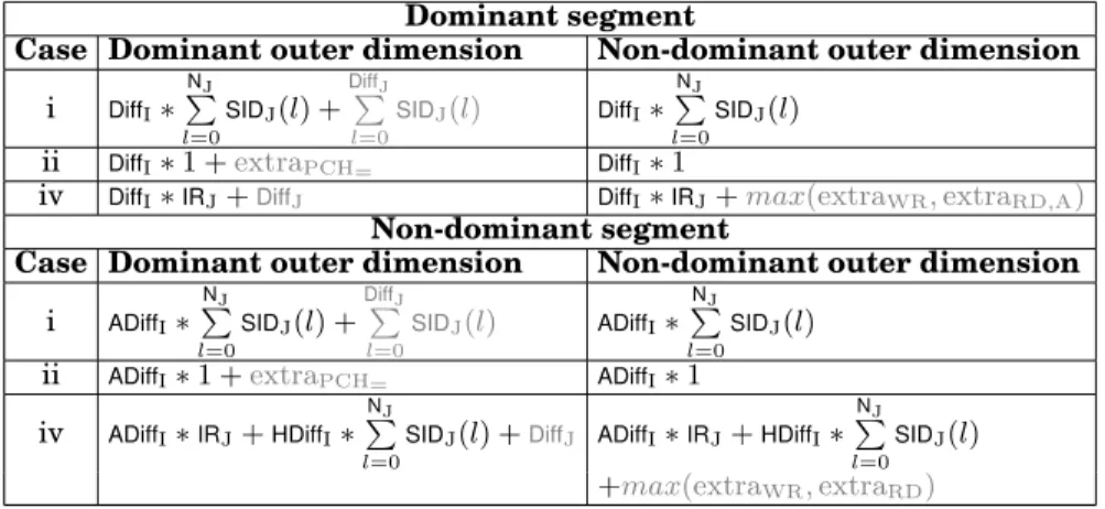
Table IV: Equations for several representative cases. The black terms describe the size due to I exploration window and the gray terms the additional elements due to J exploration window
Dominant segment
Case Dominant outer dimension Non-dominant outer dimension
i DiffI∗ NJ P l=0 SIDJ(l) + DiffJ P l=0 SIDJ(l) DiffI∗ NJ P l=0 SIDJ(l)
ii DiffI∗ 1 +extraPCH= DiffI∗ 1
iv DiffI∗IRJ+DiffJ DiffI∗IRJ+max(extraWR, extraRD,A)
Non-dominant segment
Case Dominant outer dimension Non-dominant outer dimension
i ADiffI∗ NJ P l=0 SIDJ(l) + DiffJ P l=0 SIDJ(l) ADiffI∗ NJ P l=0 SIDJ(l)
ii ADiffI∗ 1 +extraPCH= ADiffI∗ 1
iv ADiffI∗IRJ+HDiffI∗ NJ
P
l=0
SIDJ(l) +DiffJ ADiffI∗IRJ+HDiffI∗ NJ
P
l=0
SIDJ(l)
+max(extraWR, extraRD)
R=1. The exploration window is 5 and 2 for I and J dimensions, respectively. The size is (2+2)*(2+1)+2=14, where (2+2) is the summation of the accesses in a pattern sec-tion of length 5, (2+1) is the summasec-tion for the accesses in dimension J and 2 is the summation of the accesses in the exploration window J.
Example 8.3. Fig. 7(e) (code in Fig. 7(f)) describes an example where the I and the J are coupled through a PCH. The I pattern has dominant segment. The condition is dominant and belongs to case ii. The final equation is given in the top-left part of Table IV. The pattern RDI is {1H 5A}, LB=-1, UB=12, IR=12, PS=6 and R=2. The exploration window is 3 for I dimension and 1 for J dimension. The number of elements is 3*1+1=4, where 3 isDiffI, 1 is the size of J dimension due the PCH condition and 1
is the additional element that needs to be stored due to DiffJ. We observe that when
B[5] is written, B[1] has not yet been read and that still needs to be stored. If in this example the exploration window J was 0, the number of elements is 3, because when B[5] is written, B[1] has already been read.
8.1.2. Non-dominant outer dimension.In contrast to the previous case, the behavior of
the pattern in the iteration after the exploration window is alwaysH. Therefore, the
termASizeiequals to zero because at least in one dimension (dimension 0) the elements
are not accessed. Several final equations for the already presented cases i and ii and for the non-dominant outer dimension are given in the top-right part of Table IV.
8.2. Non-dominant conditions
In the case of the non-dominant conditions, at least an access in one pattern of a di-mension is enough to access the element.
(1) the termSizei depends on the type of the segment:
(a) Dominant segment: all elements are accesses in the 0 dimension and thus the size is given by the complete size of i dimension,IRi.
(b) Non-Dominant segment: even if a hole exists in 0 dimension, the element is still accessed due to the access occurring in the i dimension. These “hidden” elements are given byHDiff0. Hence, the size derives by multiplyingADiff0 with