On the clear sky model of the ESRA - European Solar Radiation Atlas with respect to the Heliosat method

HAL Id: hal-00361373

https://hal.archives-ouvertes.fr/hal-00361373

Submitted on 13 Feb 2009

HAL is a multi-disciplinary open access

archive for the deposit and dissemination of

sci-entific research documents, whether they are

pub-lished or not. The documents may come from

teaching and research institutions in France or

abroad, or from public or private research centers.

L’archive ouverte pluridisciplinaire HAL, est

destinée au dépôt et à la diffusion de documents

scientifiques de niveau recherche, publiés ou non,

émanant des établissements d’enseignement et de

recherche français ou étrangers, des laboratoires

publics ou privés.

Radiation Atlas with respect to the Heliosat method

Christelle Rigollier, Olivier Bauer, Lucien Wald

To cite this version:

Christelle Rigollier, Olivier Bauer, Lucien Wald. On the clear sky model of the ESRA - European

Solar Radiation Atlas with respect to the Heliosat method. Solar Energy, Elsevier, 2000, 68 (1),

pp.33-48. �hal-00361373�

ON THE CLEAR SKY MODEL OF THE ESRA - EUROPEAN SOLAR

RADIATION ATLAS WITH RESPECT TO THE HELIOSAT METHOD

Rigollier Christelle, Bauer Olivier, Wald Lucien Groupe Télédétection & Modélisation, Ecole des Mines de Paris

BP 207, 06904 Sophia Antipolis cedex, France Tel.: +33 (0) 4.93.95.74.49 Fax: +33 (0) 4.93.95.75.35

e-mail : lucien.wald@cenerg.cma.fr

ABSTRACT. This paper presents a clear-sky model, which has been developed in the framework of the new

digital European Solar Radiation Atlas (ESRA). This ESRA model is described and analysed with the main objective of being used to estimate solar radiation at ground level from satellite images with the Heliosat method. Therefore it is compared to clear-sky models that have already been used in the Heliosat method. The diffuse clear-sky irradiation estimated by this ESRA model and by other models has been also checked against ground measurements, for different ranges of the Linke turbidity factor and solar elevation. The results show that the ESRA model is the best one with respect to robustness and accuracy. The r.m.s. error in the estimation of the hourly diffuse irradiation ranges from 11 Wh.m-2 to 35 Wh.m-2 for diffuse irradiation up to 250 Wh.m-2. The good results obtained with such a model are due to the fact that it takes into account the Linke turbidity factor and the elevation of the site, two factors that influence the incoming solar radiation. In return, it implies the knowledge of these factors at each pixel of the satellite image for the application of the Heliosat method.

1. Introduction

In the course of the realisation of the first edition of the new digital European Solar Radiation Atlas for years 1981 - 1990 (ESRA, 1999), new models have been devised for the computation of the irradiance and further of the irradiation for clear skies. Compared to the model used for the European Solar Radiation Atlas for years 1966 - 1975 (1984), there is an explicit expression for both the beam and the diffuse components. The parameters of these models have been empirically adjusted by fitting techniques using hourly measurements spanned over several years and for several locations in Europe. The Linke turbidity factor is a key point in these models. It is a

function of the scattering by aerosols and the absorption by gas, mainly water vapour. When combined with the atmosphere molecules scattering, it summarises the turbidity of the atmosphere, and hence the attenuation of the direct beam and the importance of the diffuse fraction. The larger the Linke turbidity factor, the larger the attenuation of the radiation by the clear-sky atmosphere. Clear-sky models are instrumental in several applications in solar energy. Of particular interest to the authors is the assessment of the solar radiation from satellite images. In the Heliosat method, one of the most known methods, the clear-sky model is a central point. Cano et al. (1986) used the model of Bourges (1979), Moussu et al. (1989) a very similar one but from Perrin de Brichambaut and Vauge (1982). The clear-sky model (Kasten model) of the 1966 - 1975 Atlas (1984) has been recently introduced in the Heliosat method by the team of the University of Oldenburg (Heinemann, personal communication). The better the clear-sky model, the better the assessment of the irradiation from satellite observations. For that reason, the authors investigated the new models proposed by the ESRA.

The present article details and comments these models, including several graphs, therefore providing a more comprehensive description of these models useful for discussing its relevance to the Heliosat method. It also discusses the differences between the concurrent models proposed by the ESRA and concludes on their relevance for the computation of either the irradiance or the irradiation. Symbols used in this paper are those recommended by the ESRA.

2. The horizontal global irradiance under cloudless skies

2.1. The beam component

In this model, the global horizontal irradiance for clear sky, Gc, is split into two parts: the direct component, Bc, and the diffuse component, Dc. Each component is determined separately. The unit for irradiance is W.m-2. The direct irradiance on a horizontal surface (or beam horizontal irradiance) for clear sky, Bc, is given by:

(

)

B

c

=

I

0

sin

ε

γ

s

exp

−

0 8662

.

T AM

L

(

2

)

m

δ

R

( )

m

( 1 )

where

•

I

0 is the solar constant, that is the extraterrestrial irradiance normal to the solar beam at the mean solar

distance. It is equal to 1367 W.m-2;

•

γ

s is the solar altitude angle.

γ

s is 0° at sunrise and sunset;

•

T

L

(AM2)

is the Linke turbidity factor for an air mass equal to 2;

•

m

is the relative optical air mass;

•

δ

R

(m)

is the integral Rayleigh optical thickness.

The quantity :

(

)

exp

−

0 8662

.

T AM

L

(

2

)

m

δ

R

( )

m

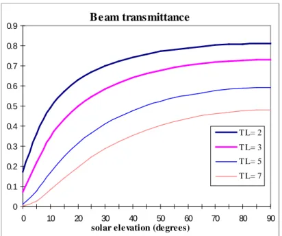
( 2 )

represents the beam transmittance of the beam radiation under cloudless skies. The relative optical air mass m expresses the ratio of the optical path length of the solar beam through the atmosphere to the optical path through a standard atmosphere at sea level with the sun at the zenith. As the solar altitude decreases, the relative optical path length increases. The relative optical path length also decreases with increasing station height above the sea level,

z

. A correction procedure is applied, obtained as the ratio of mean atmospheric pressure,

p

, at the site elevation, to mean atmospheric pressure at sea level,

p

0. This correction is particularly important in mountainous

areas. The relative optical air mass has no unit; it is given by Kasten and Young (1989), where

γ

strueis in degrees:

(

)

1.6364 -true s true s 0 true s

)

07995

.

6

+

(

50572

.

0

sin

p

p

)

(

m

γ

γ

γ

+

=

( 3 )

with the station height correction given by:

p p

0

=

exp(

−

z z

h

)

( 4 )

where

z

is the site elevation and

z

h is the scale height of the Rayleigh atmosphere near the Earth surface, equal to

8434.5 meters.

The solar altitude angle used in equation 3,

γ

s true

,is corrected for refraction:

γ

s true

(

)

(

)

(

)

(

)

(

)

∆γ

refr S S S S

=

+

+

+

+

0 061359 180

0 1594 1 1230

180

0 065656

180

1 28 9344

180

277 3971

180

2 2 2 2

.

/

.

.

/

.

/

.

/

.

/

π

π

γ

π

γ

π

γ

π

γ

( 6 )

The Rayleigh optical thickness, δR, is the optical thickness of a pure Rayleigh scattering atmosphere, per unit of air mass, along a specified path length. As the solar radiation is not monochromatic, the Rayleigh optical thickness depends on the precise optical path and hence on relative optical air mass,

m

. The parametrisation used is the following (Kasten, 1996):









+

=

°

<

>

−

+

−

+

=

°

≥

≤

m

718

.

0

4

.

10

)

m

(

1

,

)

1.9

(

20

m

if

m

00013

.

0

m

00650

.

0

m

12020

.

0

m

75130

.

1

62960

.

6

)

m

(

1

,

)

1.9

(

20

m

if

R s 4 3 2 R s

δ

γ

δ

γ

_{( 7 )}

The discrepancy between both formula at

m=20

is equal to 1.6.10-2, which is negligible (less than 0.1 per cent of

1/

δ

R

(m)

).

All the variation of the beam transmittance with air mass is included in the product m

δ

R

(m).

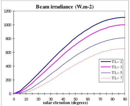
Figure 1 displays

the beam transmittance (Fig. 1.a.) and irradiance (Fig.1.b.) for

p=p

0 (sea level), and for different values of

turbidity factor (TL(AM2) = 2, 3, 5, 7), as a function of solar elevation.

2.2. The diffuse component

The diffuse irradiance falling on a horizontal surface for clear sky (or diffuse horizontal irradiance), Dc, also depends on the Linke turbidity factor, TL(AM2), at any solar elevation. In fact, the proportion of the scattered energy in the atmosphere increases as the turbidity increases, and as the beam irradiance falls, the diffuse irradiance normally rises. At very low solar altitudes and high turbidity, however, the diffuse irradiance may fall with turbidity increase due to high overall radiative energy loss in the atmosphere associated with long path length. Thus, the diffuse horizontal irradiance,

D

c, is determined by:

(

)

(

)

(

)

In this equation, the diffuse radiation is expressed as the product of the diffuse transmission function at zenith (i.e. sun elevation is 90°),

T

rd

,

and a diffuse angular function,

F

d.

(

)

(

)

(

)

[

(

)

]

T

rd

T AM

L

2

1 5843 10

3 0543 10

T AM

L

2

3 797 10

T AM

L

2

2 2 4 2

= −

_.

_.

−

+

_.

_.

−

+

_.

_.

− _{( 9 )}

For very clear sky, the diffuse transmission function is very low: there is almost no diffusion, but by the air molecules. As the turbidity increases, the diffuse transmittance increases while the direct transmittance decreases.

Typically,

T

rd ranges from 0.05 for very clear sky (

T

L

(AM2)=2

) to 0.22 for very turbid atmosphere

(

T

L

(AM2)=7

). Figure 2 displays

T

rd as a function of

T

L

(AM2)

.

The diffuse angular function,

F

d

,

depends on the solar elevation angle and is fitted with the help of second order

sine polynomial functions:

(

)

( )

[

( )

]

F

_d

γ

_s

,

T

_L

(

AM

2

)

=

A

₀

+

A

₁

sin

γ

_s

+

A

₂

sin

γ

_s 2 ( 10 )

The coefficients

A

0

, A

1

,

and

A

2, only depend on the Linke turbidity factor. They are unitless and are given by:

(

)

[

(

)

]

(

)

[

(

)

]

(

)

[

(

)

]

A

T AM

T AM

A

T AM

T AM

A

T AM

T AM

L L L L L L 0 1 2 3 2 1 2 2 2 2 2 3 2

2 6463 10

6.158110

2

3 1408 10

2

2 0402 1 8945 10

2

1 116110

2

1 3025

3 923110

2

8 5079 10

2

=

−

+

=

+

−

= −

+

+











− − − − − − −

.

.

.

.

.

.

.

.

( 11 ) with a condition on

A

0:

(

)

if A T

0 rd

A

T

rd 3 0 3

2 10

2 10

.

<

.

−

,

=

.

− ( 12 )

This condition is required because

A

0 yielded negative values for

T

L

(AM2)>6.

It was therefore decided to

The diffuse function is represented in figure 3. One can note that

F

d is not exactly equal to 1 for

γ

S

= 90°.

Equation 8 suggests that this should be the case, whatever the turbidity. The model can be improved on that point.

Once

F

d computed, the diffuse horizontal irradiance,

D

c can be determined. It is displayed in figure 4 for several

Linke turbidity factors, as a function of the solar elevation.

D

c clearly increases as the turbidity increases, due to

the increase in scattering by the aerosols. As already mentioned, it may be the opposite at very low solar altitudes and high turbidity.

Then, the direct and diffuse irradiances under cloudless sky conditions can be summed to yield the global clear sky horizontal irradiance, which is represented in figure 5. :

G

c

= B

c

+ D

c ( 13 )

The global irradiance decreases as the turbidity increases and as the solar elevation decreases. It is not equal to 0 at sunset or sunrise because of the diffuse component which is still noticeable while the sun is below the horizon.

3. The horizontal global irradiation under cloudless skies

3.1. The beam component

Once

m

,

T

L

(AM2)

,

and

δ

R

(m)

are known, the cloudless beam horizontal irradiation can be evaluated for any part

of the day by numerical integration of

B

c using suitable time steps. The site, however, may be partially

obstructed and/or the beam may not shine on a certain surface of interest for part of the time period inspected. Using a range of techniques, like shading masks on solar charts, it is possible to identify the periods of day during which the beam will actually reach the surface. The numerical integration can be adjusted for this, but the task becomes easier if the solutions can be assessed analytically rather than numerically. Thus the beam irradiance has been constructed by data fitting techniques to provide a

T

L

(AM2)

-dependent output that can be

(

)

(

)

(

)

B

_c

=

I

₀

ε

T

_rb

T

_L

AM

2

F

_b

γ

_s

,

T

_L

(

AM

2

)

( 14 )

where

T

rb

(T

L

(AM2))

is a transmission function for beam radiation at zenith and

F

bis a beam angular function.

B

c is set to 0 if equation 14 leads to a negative value. The computation of

T

rbis made at zenith, i.e. sun elevation

is 90°. So, in this case the relative optical air mass m is given by

p/p

0. Thus,

T

rb is only dependent on the Linke

turbidity factor for air mass 2 and on

p/p

0 which is determinated by the site elevation:

(

)

(

)

[

]

T

_rb

T AM

_L

2

=

exp

−

0 8662

.

T AM

_L

(

2

) (

p p

₀

)

δ

_R

(

p p

₀

)

( 15 )

F

b

(

γ

S

, T

L

(AM2))

has the form of a second order polynomial on the sine of the solar altitude,

γ

s, with coefficients

solely dependent on

T

L

(AM2)

:

(

)

( )

[

( )

]

F

b

γ

s

,

T

L

(

AM

2

)

C

0

C

1

sin

γ

s

C

2

sin

γ

s 2

=

+

+

( 16 )

Equation 14 corresponds to a re-writing of the beam irradiance, using the form used for the diffuse irradiance (equation 8).

Setting

F

b

(

γ

S

, T

L

(AM2))

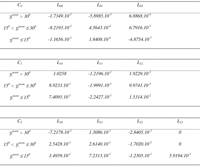
to 0 or very close to 0 may produce negative values at high turbidities. This situation

which arises only at very low altitudes, results because the polynomials are not a perfect fit. To increase the accuracy of the fits at very low solar elevation, the values of the coefficients

C

0,

C

1 and

C

2 were computed for

three ranges of the solar altitude angle at noon,

γ

s noon

: below 15°, between 15° and 30°, and over 30°. Thus the polynomials take the form:

(

)

[

(

)

]

(

)

[

(

)

]

(

)

[

(

)

]

[

(

)

]

C

L

L T AM

p p

L

T

AM

p p

C

L

L T AM

p p

L

T AM

p p

C

L

L T

AM

p p

L

T

AM

p p

L

T AM

p p

L L L L L L L 0 00 01 0 02 0 2 1 10 11 0 12 0 2 2 20 21 0 22 0 2 23 0 3

2

2

2

2

2

2

2

=

+

+

=

+

+

=

+

+

+













(

)

/

(

)

/

(

)

/

(

)

/

(

)

/

(

)

/

(

)

/

( 17 )

with the

L

ij coefficients listed in Table 1 below for the three considered ranges. These coefficients, as well as

C

i,

Finally, the analytical integral of the beam irradiation for a period ranging from solar hour angles

ω

1 to

ω

2, takes the form:

(

)

(

)

(

)

B

c

(

ω ω

,

)

I

ε

rb

T

L

AM

F

b

γ

S

,

T

L

(

AM

)

π

ω

ω ω 1 2 0

2

2

1 2

=

T

∫



_



Dl



_



2

d

( 18 )

where

Dl

is the length of the day, i.e. 24 hours or 86400 seconds,

and

ω

1 to

ω

2 are solar angles related to two instants t1 and t2 (expressed in decimal hour), according to the following equations:

ω

1

= (t

1

-12)

π

/12

ω

2

= (t

2

-12)

π

/12

( 19 )

The solar hour angle, ω, expresses the time of the day in terms of the angle of rotation of the Earth about its axis from its solar noon position at a specific place. As the Earth rotates of 360° (or 2π rad) in 24 hours, in one hour the rotation is 15° (or π/12 rad).

The unit of

B

c

(

ω

1

,

ω

2

)

is Wh.m-2 if the length of the day is expressed in hours, or J.m-2 if

Dl

is expressed in

seconds. In this equation,

(

)

F

_b

γ

_s

,

T

_L

(

AM

2

)

=

C + C

_{0 1}

sin

γ

_s

+

C

₂

sin ²

γ

_{s ( 20 )}

and can be re-written

(

)

( )

F

b

ω

, , ,

Φ

δ

T

L

(

AM

2

)

=

B + B

0 1

cos

ω

+

B

2

cos

2

ω

( 21 )

sin

γ

_s

=

sin

Φ

.sin

δ

+

cos

Φ

.cos .cos

δ

ω

( 22 ) It comes

(

)

(

)

[

]

B

c

(

ω ω

,

)

ε

Dl

_π

T

rb

T AM

L

B

ω

B

sin( )

ω

B

sin(

ω

)

_ω ω 1 2 0 1 2

2

2

2

1 2

=

I

0



_





_



+

+

( 23 )

with the coefficients

B

0,

B

1 and

B

2 given by:

[

] [

]

[

] [

]

[

] [

]

B

C

C

C

B

C

C

B

0 0 1 2 2 2 2 2 2 1 1 2 2 2 2 2

0 5

2

0 25

=

+

+

+

=

+

=













sin(

) sin( )

sin(

)

sin( )

.

cos(

)

cos( )

cos(

) cos( )

sin(

) sin( ) cos(

) cos( )

.

cos(

)

cos( )

Φ

Φ

Φ

Φ

Φ

Φ

Φ

δ

δ

δ

δ

δ

δ

δ

C

C

( 24 )

where

Φ

is the latitude of the site (positive to the Northern Hemisphere) and

δ

is the declination (positive when the sun is north to the equator: March 21 to September 23). Maximum and minimum values of the declination are +23°27' and -23°27'.

The

B

i coefficients only depend on latitude,

Φ

, and declination at noon,

δ

. The transmission function

T

rb, and the

C

i coefficients only depend on the Linke turbidity factor for air mass 2. Thus all these factors can be computed

only once for each day.

The daily integral is achieved by setting ω1 equal to the sunrise hour angle, ωSR, and ω2 to the sunset hour angle, ωSS, i.e.:

B

cd

=

B

c

(

ω ω

SR

,

SS

)

( 25 )

The daily sum of beam irradiation at different latitudes (30° and 60°),

B

cd, is displayed in figure 6 for various

turbidities, as a function of the julian day. The daily sum decreases as the turbidity increases. The distribution over the year of the daily sum is more peaked as the latitude increases, and also as the turbidity decreases.

The diffuse horizontal irradiation,

D

c

(

ω

1

,

ω

2

)

,

is computed by the analytical integration of the diffuse irradiance

(equation 8) over any period defined by

ω

1and

ω

2,and is equal to:

(

)

(

)

[

]

D

_c

(

ω ω

,

)

I

ε

Dl

T

_rd

T AM

_L

D

D

sin( )

D

sin(

)

π

ω

ω

ω

ωω 1 2 0 0 1 2

2

2

2

1 2

=



_









₊

₊

( 26 )

with the coefficients D0, D1 and D2 given by:

[

] [

]

[

] [

]

[

] [

]

D

A

A

A

D

A

A

D

0 0 1 2 2 2 2 2 2 1 1 2 2 2 2 2

0 5

2

0 25

=

+

+

+

=

+

=













sin(

) sin( )

sin(

)

sin( )

.

cos(

)

cos( )

cos(

) cos( )

sin(

) sin( ) cos(

) cos( )

.

cos(

)

cos( )

Φ

Φ

Φ

Φ

Φ

Φ

Φ

δ

δ

δ

δ

δ

δ

δ

A

A

( 27 )

where the

A

i coefficients only depend on the Linke turbidity factor for air mass 2 and have been given previously

(equation 11).

The daily integral is achieved by setting ω1 equal to the sunrise hour angle, ωSR, and ω2 to the sunset hour angle, ωSS, i.e.

D

_cd

=

D

_c

(

ω ω

_SR

,

_SS

)

( 28 )

The daily sum of diffuse irradiation at different latitudes (30° and 60°),

D

cd, is displayed in figure 7 for various

turbidities, as a function of the julian day. The daily sum increases as the turbidity increases. The distribution over the year of the daily sum is more peaked as the latitude increases, and also as the turbidity increases.

3.3. Are both formulations equivalent ?

For each component of the irradiance, two empirical formulations have been proposed in sections 2 and 3. The first one (section 2) has been investigated for the assessment of irradiance (W.m-2), and gives instantaneous values of solar radiation. The second one (section 3) is more suitable to compute irradiation (Wh.m-2), since it

during appropriate time period (for instance one hour, or one day) in order to compute irradiation. To integrate irradiance, the method presented in section 3 decomposes both the beam and the diffuse components using transmission functions and solar angular functions. Irradiation can also be computed by numerical integration of the formulation of section 2 using fitting time steps. But, as discussed in section 3.1, an analytical integration is easier to handle than a numerical one.

Both formulations have been compared for the computation of the clear-sky beam horizontal irradiance (equations 1 and 14). Figure 8 displays both models for beam irradiance. The differences are small, they do not exceed 18 W.m-2 as shown in figure 9 and are less than 3 % for solar elevation above 25°. The diffuse irradiance has the same formulation in both sections. Therefore, the difference between the global irradiance in section 2 and section 3 is given by the difference between beam irradiances. Both formulations lead to very similar results and should be considered as equivalent for the assessment of the beam irradiance. Therefore, to compute the irradiation, the easiest-to-compute formulation should be preferred. The formulation of section 3 is the simplest and should be used to compute clear-sky irradiation.

3.4. The global irradiation

The sky global irradiation is obtained as the sum of the sky beam horizontal irradiation and the clear-sky diffuse horizontal irradiation between two instants t1 and t2, according to the equation 19.

G

c

(

ω

1

,

ω

2

) = B

c

(

ω

1

,

ω

2

) + D

c

(

ω

1

,

ω

2

)

( 29 )

The parameters

ω

1 and

ω

2 are respectively set to

ω

SR and

ω

SS for the computation of the daily sum of clear sky

global irradiation:

G

c

(

ω

SR

,

ω

SS

) = B

c

(

ω

SR

,

ω

SS

) + D

c

(

ω

SR

,

ω

SS

)

( 30 )

⇔

G

cd

= B

cd

+ D

cd ( 31 )

The daily sum of global irradiation at different latitudes (30° and 60°),

G

cd

,

is displayed in figure 10 for various

turbidities, as a function of the julian day. The daily sum decreases as the turbidity increases. The distribution over the year of the daily sum is more peaked as the latitude increases, and also as the turbidity decreases.

4. Comparison with other clear-sky models

4.1. Comparison with clear-sky models used previously in the Heliosat method

In the original version of the Heliosat method, Cano et al. (1986) used the model of Bourges (1979) to obtain the global irradiance under clear-sky:

G

c (Bourges)

= 0.70 I

0

ε

(sin

γ

S

)

1.15 _{( 32 )}

Figure 11 displays the global irradiances for this model and the ESRA model. Four different values of the Linke turbidity factor have been used: 2, 3, 5, and 7. When the solar elevation is low, both models give similar results. But when the solar elevation becomes higher than 30°, the values given by the model of Bourges are close to the values given by the ESRA model for a Linke turbidity factor between 5 and 7. Yet, in Europe, the average Linke turbidity factor is about 3.5. Therefore, the global irradiance estimated by the model of Bourges is too low for Europe, as a general rule.

The global clear-sky irradiance given by the model of Perrin de Brichambaut and Vauge (1982), hereafter noted PdBV, was used by Moussu et al. (1989) in their study on the Heliosat method. This model is very similar to the model of Bourges, and is given by:

G

c (PdBV)

= 0.81 I

0

ε

(sin

γ

S

)

1.15 _{( 33 )}

This model, as well as that of Bourges, does not explicitly take into account the aerosols, the water content, nor the ground albedo. To check the validity of this model, Moussu et al. compare it to the clear-sky model described by Iqbal (1983, model C) after the works of Bird and Hulstrom (1981 a, b) for various values of ground albedo, precipitable water thickness, and horizontal visibility. The comparison demonstrates that the shape of the model PdBV is consistent with the model C and that the variation of Gc is well described by the function (sin γS)0.15. However the magnitude of Gc (PdBV) suffers from the lack of input parameters. Figure 11 displays also the PdBV model. One can note that for a Linke turbidity factor equal to 3, the ESRA and PdBV models give very similar values of the clear-sky global irradiance for all range of solar elevation.

Both models, Gc (Bourges) and Gc (PdBV) have been useful to establish the Heliosat method for the assessment of the solar radiation and ground albedo. However their lack of accuracy prevents from further improvements in the Heliosat method. A more accurate model is needed which includes other parameters, such as the Linke turbidity factor and the elevation. A first step was made by Iehlé et al. (1997) who established that the introduction of the ESRA model in the Heliosat method would result into an increase of the accuracy of the estimates. They briefly examined the models of Kasten (European Solar Radiation Atlas, 1984) and of Dumortier (1995) on purely analytical grounds. They concluded that within Heliosat both models should lead to slightly larger mean bias errors than the ESRA model. Iehlé et al. only used one year of data for four stations in Europe. In the course of the Satellight programme funded by the European Commission (Fontoynont et al., 1998), it was also concluded that the use of the Linke turbidity factor increases the accuracy of the estimates made by the Heliosat method. In this Satellight version of the Heliosat method, the clear-sky model is the one of Dumortier. Similar findings on the benefit of introducing TL(AM2) were made by Rigollier and Wald (1999).

4.2. Comparison with other models

Other models taking into account the Linke turbidity factor and ground elevation have been compared to the ESRA model. The clear-sky irradiance given in the WMO document 557 (1981, page 124) is:

G

c

= (1297 - 57 T

L

(AM2)) (sin

γ

S

)

[(36 + TL(AM2))/33] _{( 34 )}

Rigollier and Wald (1999) show that it provides similar results to the ESRA model. They also rise doubts on the equation for diffuse component which does not behave properly at low solar elevations (below 10° - 15°) and overestimates the diffuse radiation. They recommended to use the ESRA model instead.

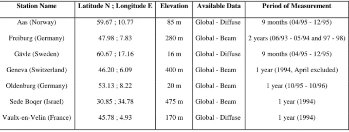
The model of Dumortier and a MODTRAN derived model have been retained for comparison with the ESRA model. The three models have in common the equation for beam radiation (equation 1). Accordingly, the comparison is restricted to the diffuse component Dc. For validation, half-hourly measurements of either global and direct, or global and diffuse irradiation were used at seven stations for different time periods (Table 2). The diffuse, or direct component is computed by the subtraction of the measured component from the global irradiation. The instantaneous Linke turbidity factor is deduced from the measurements using equation 1 and assuming that the half-hourly irradiation can be assimilated to the irradiance:

T

L

(AM2) = - ln(B

c

/ I

0

ε

sin

γ

S

) / 0.8662

δ

R

(m) m

( 35 )

Non clear-skies are then excluded from the measurements by excluding large values of TL(AM2). In fact, two thresholds were used, ranging from 2.0 to 6.5, defining fifteen TL(AM2) intervals, partly overlapping each other, in order to check the influence of such choices on the conclusions : [2.0 - 3.5], [2.5 - 3.5], [3.0 - 3.5], [2.0 - 4.0], [2.5 - 4.0], [3.0 - 4.0], [2.0 - 5.0], [2.5 - 5.0], [3.0 - 5.0], [2.0 - 6.0], [2.5 - 6.0], [3.0 - 6.0], [2.0 - 6.5], [2.5 - 6.5], [3.0 - 6.5]. The remaining measurements were then compared to the three models of diffuse irradiance. This irradiance is also assimilated to the half-hourly irradiation for the comparison.

The model of Dumortier (1995) is defined only for solar elevation angles lower than 70°, and is given by the following expression:

D

c

= I

0

ε

(0.0065 + (-0.045 + 0.0646 T

L

(AM2)) sin

γ

S

- (-0.014 + 0.0327 T

L

(AM2)) sin²

γ

S

)

( 36 )

with the conditions: γS < 70° and 2,5 ≤ TL(AM2) ≤ 6,5.

The third model was developed at the University of Oldenburg (Beyer et al., 1997) using the radiative transfer code MODTRAN 3.5 (Kneizys et al., 1996). Various simulations were made using various sets of parameters. The following expression was found to well fit the outputs of MODTRAN:

D

c

= I

0

ε

(a + b T

L

(AM2) + c T

L

(AM2)

2

+ (d + e T

L

(AM2) + f T

L

(AM2)

2

) sin

γ

S

+

(g + h T

L

(AM2) + i T

L

(AM2)

2

) sin²

γ

S

)

( 37 ) a = 0.017991 d = -0.112593 g = -0.019104 b = -0.003967 e = 0.101826 h = -0.022103 c = 0.000203 f = -0.006220 i = 0.003107

Figure 12 displays these three models for a Linke turbidity factor of 3 and 6. These models are quite similar for low solar elevation and diverge at high elevation.

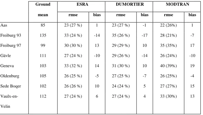
For each remaining measurement, the three models were performed using the corresponding half-hourly TL(AM2) value. The differences between the model estimates and the observations were computed and then

summarised as bias (estimates mean minus observations mean) and root mean square error (rmse) for each range of TL(AM2) and some ranges of solar elevation (Table 3).

When comparing the different models, the results obtained show that the three clear-sky models give similar results. None of the models always gives the best results. However, one can note that the ESRA clear-sky model never gives the worse errors. Therefore it may be considered as the most robust of the three models. This property is a key point when automatic processing of large volumes of data is at stake. For this reason, the ESRA clear-sky model should be preferred. For this model, the rmse is comprised between 11 and 35 Wh.m-2, for all ranges of TL(AM2) for diffuse irradiation up to 250 Wh.m

-2

. There is no significant dependence of the results on the geographical location and on the ground elevation. The results obtained for Freiburg, where two datasets of one year are available, show a high temporal variability.

We have validated these conclusions with another dataset of seven stations which is more expanded in time : from 1981 to 1990, but it offers a lower geographical coverage (Table 4). This dataset is extracted from the ESRA. Uccle offers half-hourly measurements of global, diffuse and beam irradiations, while only hourly sums of global and diffuse irradiation are available for the other stations.

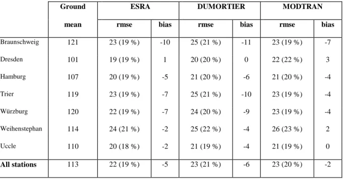
The results computed over ten years show that even if the errors are similar for the three models, the ESRA model always gives the best results for all stations when considering average errors over the ten years. In Tables 5 and 6 are reported root mean square errors (rmse) and bias for the three models, and for two ranges of TL(AM2).

The results are slightly the same for the different sites. There is still no significant dependence of the results on ground elevation or geographical location. Moreover, the differences in error observed in 1994 between two remote sites such as Sede Boqer and Vaulx-en-Velin are not higher than those observed between 1981 and 1990 for the different German stations. This low spatial variability allows to conclude that the model is not affected by the climate. The high temporal variability noted for Freiburg between results in 1993 or in 1997 is also observed for this ten-years dataset. For example, for a Linke turbidity factor ranging from 2 to 3.5, rmse of the ESRA model are varying from 11 to 18 Wh.m-2 in Hamburg while the ten-years error is 15 Wh.m-2. In Weihenstephan, rmse are varying from 14 to 25 Wh.m-2 while the ten-years error is 19 Wh.m-2. Half-hourly values are available

for Uccle, therefore a computation has been made to get hourly values in order to compare errors obtained from these two kinds of data. Similar numbers are observed for the assessment of the irradiation on hourly basis than those obtained from half-hourly basis.

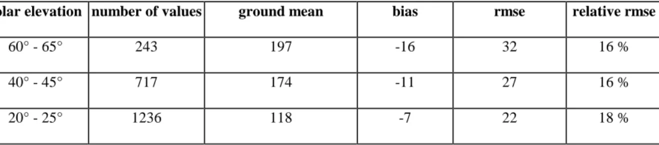
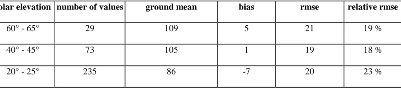
Tables 7 and 8 report values of rmse, relative rmse, and bias for the ESRA model and selected solar elevations: 20° ≤ γS ≤ 25°, 40° ≤ γS ≤ 45°, and 60° ≤ γS ≤ 65°. These tables have been drawn for Würzburg, but are representative of the other German stations since there is no climate effect. On the one hand, there is no clear dependence on the solar elevation within the results, even if the errors are varying from one range to another. On the other hand, these tables illustrate the importance of the selection of the range of TL(AM2) on the results. The rmse in Wh.m-2 decreases when skies are getting clearer. This holds for all models and all ranges of solar elevation and numbers should be considered with care. However the conclusions drawn are valid for all ranges of TL(AM2).

In this study, equation 1 was used to compute TL(AM2) for the sake of the simplicity. If the second formulation (equation 14) had been used, it would have resulted in slightly different TL(AM2) values but similar errors than the first formulation.

5. Conclusion

We have analysed the models proposed by the new digital European Solar Radiation Atlas (ESRA) for the assessment of the irradiance and the irradiation under clear sky for both the beam and the diffuse components. We have investigated the variations of these models with various parameters, namely the sun elevation and the Linke turbidity factor. The ESRA proposes two sets of models. One is best suited for the assessment of the irradiance. The other should be preferred for the computation of hourly irradiation and daily sum of irradiation. We conclude that these models can be used in the framework of the Heliosat method, especially the second one, since the aim of the Heliosat method is to estimate solar irradiation received at ground level from satellite images.

The ESRA model has been compared to several other clear-sky models and has proved to be the most accurate as a whole, though other models lead to similar results.

Compared to the other models used up to now in the Heliosat method, the accuracy in the ESRA model is mostly gained by the introduction of the Linke turbidity factor. From an operational point of view, the use of the ESRA

model implies the knowledge at each pixel of the image, of the Linke turbidity factor and of the ground elevation.

Digital maps of ground elevation are currently available for the whole Earth with a spatial resolution suitable for the processing of images from the meteorological satellites. Accuracy elevation may be questioned in several parts of such maps. However the impact of this accuracy on the outputs of the ESRA model is less than the impact of an error on TL(AM2). This factor is hardly known everywhere and an effort should be devoted to its assessment at each pixel of the image, at least on a climatological basis, season by season.

These models have been coded in language C and should be available as sources at the WWW site Helioserve: www-helioserve.cma.fr/. In this site, user can already simulate the clear-sky irradiation, given the geographical site, the elevation and the Linke turbidity factor. A database of the Linke turbidity factor has also been set up for about 700 sites. These values are available in this WWW site and can be used for a better assessment of the clear-sky radiation (Angles et al., 1998).

6. Acknowledgements

The content of the present paper was influenced by some chapters of the ESRA handbook. Fruitful discussions with John Page (Sheffield, United Kingdom) have helped to improve the clearness of this article. The authors deeply acknowledge the help of the University of Oldenburg (Germany); part of this work was made there using their valuable softwares and databases. This work was partly supported by the programme JOULE of the European Commission (DGXII): programmes ESRA (co-ordinator: K. Scharmer, GET, Germany) and SatelLight (co-ordinator: M. Fontoynont, ENTPE, France).

7. References

Angles J., Menard L., Bauer O., Wald L. (1998) A Web server for accessing a database on solar radiation parameters. In Proceedings of the Earth Observation & Geo-Spatial Web and Internet Workshop '98, Josef Strobl & Clive Best (Eds), Salzburger Geographische Materialien, Universität Salzburg, Salzburg, Austria, Heft 27, pp. 33-34.

Beyer H.G., Hammer A., Heinemann D., Westerhellweg A. (1997) Estimation of diffuse radiation from Meteosat data. North Sun ’97, 7th International Conference on Solar Energy at High Latitudes, Espoo-Otaniemi.

Bird R. and Hulstrom R. L. (1981 a) Direct insolation models, Transactions of the ASME Journal Solar Energy

Engineering, 103, 182-192.

Bird R. and Hulstrom R. L. (1981 b) A simplified clear sky model for direct and diffuse insolation on horizontal surfaces. Report SERI/TR-642-761, Solar Energy Research Institute, Golden, Colorado, U.S.A.

Bourges G. (1979) Reconstitution des courbes de fréquence cumulées de l’irradiation solaire globale horaire reçue par une surface plane. Report CEE 295-77-ESF of Centre d’Energétique de l’Ecole Nationale Supérieure des Mines de Paris, tome II, Paris, France.

Cano D., Monget J.M., Albuisson M., Guillard H., Regas N. and Wald L. (1986) A method for the determination of the global solar radiation from meteorological satellite data. Solar Energy, 37, 31-39.

Dumortier D. (1995) Modelling global and diffuse horizontal irradiances under cloudless skies with different turbidities. Final report JOU2-CT92-0144, Daylight II. Ecole Nationale des Travaux Publics de l’État, Vaulx-en-Velin, France.

ESRA (1999) European solar radiation atlas. Fourth edition, includ. CD-ROM. Edited by J. Greif, K. Scharmer. Scientific advisors: R. Dogniaux, J. K. Page. Authors : L. Wald, M. Albuisson, G. Czeplak, B. Bourges, R. Aguiar, H. Lund, A. Joukoff, U. Terzenbach, H. G. Beyer, E. P. Borisenko. Published for the Commission of the European Communities by Presses de l'Ecole, Ecole des Mines de Paris, Paris, France.

European Solar Radiation Atlas. Second Improved and Extended Edition, Vols. I and II. (1984) W. Palz (Ed.).

Commission of the European Communities, DG Science, Research and Development, Report No. EUR 9344, Bruxelles.

Fontoynont M., Dumortier D., Heinemann D., Hammer A., Olseth J., Skartveit A., Ineichen P., Reise C., Page J., Roche L., Beyer H.-G., Wald L. (1998) Satellight: a WWW server which provides high quality daylight and solar radiation data for Western and Central Europe. In Proceedings of the 9th Conference on Satellite

Meteorology and Oceanography. Published by Eumetsat, Darmstadt, Germany, EUM P 22, pp. 434-435.

Iehlé A., Lefèvre M., Bauer O., Martolini M. and Wald L. (1997) Meteosat: A valuable tool for agro-meteorology, Final Report for the European Commission, Joint Research Center, Ispra, Italy.

Iqbal M. (1983) An introduction to Solar Radiation (New York: Academic Press), pp. 107-169.

Kasten F. and Young A.T. (1989) Revised optical air mass tables and approximation formula. Applied Optics, 28 (22), 4735-4738.

Kasten F. (1996) The Linke turbidity factor based on improved values of the integral Rayleigh optical thickness.

Solar Energy, 56, 239-244.

Kneizys F. X. et al. (1996) The MODTRAN 2/3 Report and LOWTRAN 7 Model. Technical Report, Phillips Laboratory, Geophysics Directorate, Hanscom AFB.

Moussu G., Diabate L., Obrecht D. and Wald L. (1989) A method for the mapping of the apparent ground brightness using visible images from geostationary satellites, Int. J. Remote Sensing, 10 (7), 1207-1225.

Page J.K. (1995) The estimation of diffuse and beam irradiance, and diffuse and beam illuminance from daily global irradiation, a key process in the evolution of microcomputer packages for the new European Solar Radiation and Daylighting Atlases. Technical Report No. 8, prepared June 30th, 1995 and revised August 6th, 1995, 37 pp. + 5 pp. of tables. Appendix 1: Solar elevation functions for estimating cloudless day beam irradiance and daily beam irradiation on horizontal surfaces from the beam transmittance, 12 pp. + 5 pp. of tables. Page, J.K., 1996. Technical Report No. 8, revised September 21st, 1996, 36 pp. + 5 pp. of tables. Appendix 1: Revised September 22nd, 1996, 13 pp + 5 pp. of tables.

Perrin de Brichambaut C. and Vauge C. (1982) Le gisement solaire : Evaluation de la ressource énergétique. (Paris : Technique et documentation (Lavoisier).

Rigollier C. and Wald L. (1999) Selecting a clear-sky model to accurately map solar radiation from satellite images. To be published in : Proceedings of the 19th EARSeL Symposium “Remote sensing in the 21st century: economic and environmental applications”, Valladolid, Spain, Nieuwenhuis G., Vaughan R., Molenaar M. (Eds), Balkema.

World Meteorological Organization, WMO (1981). Meteorological aspects of the utilization of solar radiation as an energy source. Annex: World maps of relative global radiation. Technical Note No. 172, WMO-No. 557, Geneva, Switzerland, 298 pp.

C

0

L

00

L

01

L

02

γ

s noon

> 30

0

-1.7349.10

-2

-5.8985.10

-3

6.8868.10

-4

15

0

<

γ

s noon

≤

30

0

-8.2193.10

-3

4.5643.10

-4

6.7916.10

-5

γ

s noon

_≤

15

0

-1.1656.10

-3

1.8408.10

-4

-4.8754.10

-7

C

1

L

10

L

11

L

12

γ

s noon

> 30

0

1.0258

-1.2196.10

-1

1.9229.10

-3

15

0

<

γ

s noon

≤

30

0

8.9233.10

-1

-1.9991.10

-1

9.9741.10

-3

γ

s noon

≤

15

0

7.4095.10

-1

-2.2427.10

-1

1.5314.10

-2

C

2

L

20

L

21

L

22

L

23

γ

s noon

> 30

0

-7.2178.10

-3

1.3086.10

-1

-2.8405.10

-3

0

15

0

<

γ

s noon

≤

30

0

2.5428.10

-1

2.6140.10

-1

-1.7020.10

-2

0

γ

s noon

≤

15

0

3.4959.10

-1

7.2313.10

-1

-1.2305.10

-1

5.9194.10

-3

Station Name Latitude N ; Longitude E Elevation Available Data Period of Measurement

Aas (Norway) 59.67 ; 10.77 85 m Global - Diffuse 9 months (04/95 - 12/95)

Freiburg (Germany) 47.98 ; 7.83 280 m Global - Beam 2 years (06/93 - 05/94 and 97 - 98)

Gävle (Sweden) 60.67 ; 17.16 16 m Global - Diffuse 9 months (04/95 - 12/95)

Geneva (Switzerland) 46.20 ; 6.09 400 m Global - Beam 1 year (1994, April excluded)

Oldenburg (Germany) 53.13 ; 8.22 20 m Global - Beam 1 year (10/95 - 10/96)

Sede Boqer (Israel) 30.85 ; 34.78 475 m Global - Beam 1 year (1994)

Vaulx-en-Velin (France) 45.78 ; 4.93 170 m Global - Diffuse 1 year (1994)

Ground ESRA DUMORTIER MODTRAN

mean rmse bias rmse bias rmse bias

Aas 85 23 (27 %) 1 23 (27 %) -1 22 (26%) 1 Freiburg 93 135 33 (24 %) -14 35 (26 %) -17 28 (21%) -7 Freiburg 97 99 30 (30 %) 13 29 (29 %) 10 35 (35%) 17 Gävle 111 27 (24 %) -10 29 (26 %) -14 26 (24%) -10 Geneva 103 33 (32 %) 14 31 (30 %) 10 40 (39%) 19 Oldenburg 105 26 (25 %) -5 27 (25 %) -7 26 (25%) -4 Sede Boqer 102 26 (26 %) 10 24 (24 %) 5 27 (27%) 15 Vaulx-en-Velin 112 27 (24 %) 6 27 (24 %) 4 33 (30%) 13

Table 3 Results in Wh.m-2 obtained when comparing the diffuse models of Dumortier, ESRA, and MODTRAN with half-hourly values. Only the values corresponding to a TL(AM2) between 2.5 and 6.5 have been retained.

Station Name Latitude N ; Longitude E

Elevation Station Name Latitude N ; Longitude E

Elevation

Braunschweig(Germany) 52.30 ; 10.45 83 m Würzburg (Germany) 49.77 ; 9.97 275 m

Dresden (Germany) 51.12 ; 13.68 246 m Weihenstephan (Germany) 48.40 ; 11.70 472 m

Hamburg (Germany) 53.65 ; 10.12 49 m Uccle (Belgium) 50.80 ; 4.35 100 m

Trier (Germany) 49.75 ; 6.67 278 m

Table 4 Description of the second dataset of ground stations. The data are measured from January 1981 to

Ground ESRA DUMORTIER MODTRAN

mean rmse bias rmse bias rmse bias

Braunschweig 79 19 (24 %) -8 22 (28 %) -15 22 (28 %) -11 Dresden 61 13 (22 %) -2 15 (25 %) -8 16 (26 %) -6 Hamburg 70 15 (22 %) -3 18 (25 %) -9 18 (25 %) -6 Trier 76 17 (22 %) -3 19 (25 %) -10 19 (25 %) -6 Würzburg 76 17 (23 %) -5 20 (27 %) -12 20 (26 %) -9 Weihenstephan 72 20 (27 %) -1 21 (29 %) -7 21 (30 %) -4 Uccle 66 16 (25 %) -1 17 (26 %) -7 18 (27 %) -4 All stations 71 17 (24 %) -3 19 (27 %) -9 19 (27 %) -7

Table 5 Results in Wh.m-2 obtained when comparing the diffuse models of ESRA, Dumortier, and MODTRAN with hourly values of the second ground dataset. TL(AM2) ranges from 2.5 and 3.5.

Ground ESRA DUMORTIER MODTRAN

mean rmse bias rmse bias rmse bias

Braunschweig 121 23 (19 %) -10 25 (21 %) -11 23 (19 %) -7 Dresden 101 19 (19 %) 1 20 (20 %) 0 22 (22 %) 3 Hamburg 107 20 (19 %) -5 21 (20 %) -6 21 (20 %) -4 Trier 119 23 (19 %) -7 25 (21 %) -10 23 (19 %) -4 Würzburg 120 22 (19 %) -7 24 (20 %) -9 23 (19 %) -4 Weihenstephan 114 24 (21 %) -2 25 (22 %) -4 26 (23 %) 2 Uccle 110 20 (18 %) -2 21 (19 %) -4 21 (19 %) 0 All stations 113 22 (19 %) -5 23 (21 %) -6 23 (20 %) -2

solar elevation number of values ground mean bias rmse relative rmse

60° - 65° 243 197 -16 32 16 %

40° - 45° 717 174 -11 27 16 %

20° - 25° 1236 118 -7 22 18 %

Table 7 Results in Wh.m-2 obtained for different ranges of solar elevation when comparing the diffuse ESRA model with hourly values measured in Würzburg (Germany). Only the values corresponding to a Linke turbidity

solar elevation number of values ground mean bias rmse relative rmse

60° - 65° 29 109 5 21 19 %

40° - 45° 73 105 1 19 18 %

20° - 25° 235 86 -7 20 23 %

Beam transmittance

0 0.1 0.2 0.3 0.4 0.5 0.6 0.7 0.8 0.9 0 10 20 30 40 50 60 70 80 90

solar elevation (degrees)

T L= 2 T L= 3 T L= 5 T L= 7

Beam irradiance (W.m-2)

0 200 400 600 800 1000 1200 0 10 20 30 40 50 60 70 80 90

solar elevation (degrees)

T L= 2 T L= 3 T L= 5 T L= 7

Diffuse transmission function at zenith, Trd

0 0.05 0.1 0.15 0.2 0.25 0.3 0 1 2 3 4 5 6 7 8 9 TL(AM2)

Diffuse angular function, Fd

0 0.2 0.4 0.6 0.8 1 1.2 0 10 20 30 40 50 60 70 80 90

solar elevation (degrees)

T L=2 T L= 3 T L= 5 T L= 7

Diffuse irradiance (W.m-2)

0 50 100 150 200 250 300 350 0 10 20 30 40 50 60 70 80 90

solar elevation (degrees) T L= 2

T L= 3 T L= 5 T L= 7

Global irradiance (W.m-2)

0 200 400 600 800 1000 1200 0 10 20 30 40 50 60 70 80 90

solar elevation (degrees)

T L= 2 T L= 3 T L= 5 T L= 7

Daily sum of be am irradiation

(Wh.m-2) at 30° latitude

0 1000 2000 3000 4000 5000 6000 7000 8000 9000 1 17 46 75 104 133 162 191 220 249 278 307 336 365 julian day T L= 2 T L= 3 T L= 5 T L= 7

Daily sum of beam irradiation

(Wh.m-2) at 60° latitude

0 1000 2000 3000 4000 5000 6000 7000 8000 9000 1 17 46 75 104 133 162 191 220 249 278 307 336 365 julian day T L= 2 T L= 3 T L= 5 T L= 7

Daily sum of diffuse irradiation

(Wh.m-2) at 30° latitude

0 500 1000 1500 2000 2500 3000 1 17 46 75 104 133 162 191 220 249 278 307 336 365 julian day T L= 2 T L= 3 T L= 5 T L= 7

Daily sum of diffuse irradiation

(Wh.m-2) at 60° latitude

0 500 1000 1500 2000 2500 3000 3500 1 17 46 75 104 133 162 191 220 249 278 307 336 365 julian day T L= 2 T L= 3 T L= 5 T L= 7

Beam irradiance (W.m-2) evaluated with both

models (§2 and §3)

0 100 200 300 400 500 600 700 800 900 0 10 20 30 40 50

solar elevation (degrees)

Bc_§3 Bc_§2 TL=2 TL=3 TL=5 TL=7

Fig. 8 Comparison between both models : Bc_§2 (section 2) and Bc_§3 (section 3) for the computation of the

beam horizontal irradiance for clear sky. The computation has been made at mean solar distance, 45° latitude and 0° longitude (the solar declination δ is equal to 5.70°, ε is equal to 1, and γS

noon

Difference [Bc (§2) - Bc (§3)] (W.m-2)

-20 -15 -10 -5 0 5 10 15 0 10 20 30 40 50

solar e le vation (de gre e s)

TL= 2 TL= 3 TL= 5 TL= 7

Fig. 9 Difference between Bc_§2 (beam irradiance for clear sky, section 2) and Bc_§3 (beam irradiance for

Daily sum of global irradiation

(Wh.m-2) at 30° latitude

0 1000 2000 3000 4000 5000 6000 7000 8000 9000 10000 1 17 46 75 104 133 162 191 220 249 278 307 336 365 julian day T L= 2 T L= 3 T L= 5 T L= 7

Daily sum of global irradiation

(Wh.m-2) at 60° latitude

0 1000 2000 3000 4000 5000 6000 7000 8000 9000 10000 1 17 46 75 104 133 162 191 220 249 278 307 336 365 julian day T L= 2 T L= 3 T L= 5 T L= 7

Global irradiance (W.m-2)

0 200 400 600 800 1000 1200 0 10 20 30 40 50 60 70 80 90

solar e le vation (de gre s)

TL= 2 TL= 3 TL= 5 TL= 7 Gc Bourges Gc PdBV Gc ESRA

Fig. 11 Comparison between the ESRA model (Gc ESRA) for different values of TL(AM2) , the model of Bourges,

Diffuse irradiances with T

L

= 3 (W.m

-2

)

0 20 40 60 80 100 120 0 10 20 30 40 50 60 70 80 90

solar elevation (degrees) Dc_ESRA Dc_DUMORTIER Dc_MODTRAN

Diffuse irradiances with T

L

= 6 (W.m

-2

)

0 50 100 150 200 250 300 350 0 10 20 30 40 50 60 70 80 90

solar elevation (degrees) Dc_ESRA Dc_DUMORTIER Dc_MODTRAN

Fig. 12 The diffuse components of the ESRA model (Dc ESRA), the DUMORTIER model (Dc Dumortier), and