Série Scientifique
Scientific Series
Montréal Octobre 1996 96s-25
How Did Ontario Pulp and Paper
Producers Respond to Effluent
Regulations, 1985-89?
Paul Lanoie, Mark Thomas,
Ce document est publié dans lintention de rendre accessibles les résultats préliminaires de la recherche effectuée au CIRANO, afin de susciter des échanges et des suggestions. Les idées et les opinions émises sont sous lunique responsabilité des auteurs, et ne représentent pas nécessairement les positions du CIRANO ou de ses partenaires.
This paper presents preliminary research carried out at CIRANO and aims to encourage discussion and comment. The observations and viewpoints expressed are the sole responsibility of the authors. They do not necessarily represent positions of CIRANO or its partners.
CIRANO
Le CIRANO est une corporation privée à but non lucratif constituée en vertu de la Loi des compagnies du Québec. Le financement de son infrastructure et de ses activités de recherche provient des cotisations de ses organisations-membres, dune subvention dinfrastructure du ministère de lIndustrie, du Commerce, de la Science et de la Technologie, de même que des subventions et mandats obtenus par ses équipes de recherche. La Série Scientifique est la réalisation dune des missions que sest données le CIRANO, soit de développer lanalyse scientifique des organisations et des comportements stratégiques.
CIRANO is a private non-profit organization incorporated under the Québec Companies Act. Its infrastructure and research activities are funded through fees paid by member organizations, an infrastructure grant from the Ministère de lIndustrie, du Commerce, de la Science et de la Technologie, and grants and research mandates obtained by its research teams. The Scientific Series fulfils one of the missions of CIRANO: to develop the scientific analysis of organizations and strategic behaviour.
Les organisations-partenaires / The Partner Organizations École des Hautes Études Commerciales.
École Polytechnique. McGill University. Université de Montréal.
Université du Québec à Montréal. Université Laval.
MEQ. MICST. Avenor.
Banque Nationale du Canada Bell Québec.
Fédération des caisses populaires de Montréal et de lOuest-du-Québec. Hydro-Québec.
La Caisse de dépôt et de placement du Québec. Raymond, Chabot, Martin, Paré
Société délectrolyse et de chimie Alcan Ltée. Téléglobe Canada.
Ville de Montréal.
Correspondence Address: Paul Lanoie, CIRANO, 2020 University Street, 25th floor, *
Montréal, Qc, Canada H3A 2A5 Tel: (514) 985-4020 Fax: (514) 985-4039 e-mail: lanoiep@cirano.umontreal.ca
We would like to thank two anonymous referees for helpful comments on a first version of this paper. École des Hautes Études Commerciales and CIRANO
Princeton University
How Did Ontario Pulp and Paper
Producers Respond to Effluent
Regulations, 1985-89?
*
Paul Lanoie , Mark Thomas , Joan Fearnley
§Résumé / Abstract
Cet article explore les effets de la réglementation des émissions de polluants sur les firmes de lindustrie ontarienne des pâtes et papier. Le modèle utilise des variables instrumentales pour faire la distinction entre les effets liés à la * capture + de lagence de réglementation et des effets vraiment propres à laction du régulateur. Le modèle cherche également à identifier les moyens utilisés par les entreprises pour faire face à la réglementation : des données sont disponibles pour les dépenses en équipement anti-pollution des entreprises et sur la quantité deau consommée. Les résultats tendent à démontrer que le contrôle des émissions polluantes se ferait de façon plus efficace par limposition dune limite sur les rejets de matières en suspension (MES) que par une limite sur la demande biochimique en oxygène. Les effets constatés sur la firme dune limite sur les MES, proviendraient en partie dune modification dans la production, qui aurait pour effet de diminuer les émissions. Par contre, les investissements en équipement anti-pollution, consentis pour atteindre les objectifs de réduction de DBO, nont eu aucun effet sur les émissions. Limpact des poursuites légales, des amendes et des enquêtes est impossible à détecter. Parmi les causes possibles de ces résultats, notons que les sanctions imposées par lOntario aux entreprises lors dune infraction sur lémission de polluant, durant la période détude, étaient trop faibles pour influencer de façon mesurable le comportement des entreprises. Une autre cause pourrait être le fait que les limites démissions sont assez élevées pour ne pas être contraignantes pour la plupart des firmes de léchantillon.
This paper explores the effects of effluent regulatory activity on firm behavior in the pulp and paper industry in Ontario. The model uses instrumental variables to attempt to distinguish between that correlation between emission limits and emissions coming from regulatory capture and that coming from true influence on the part of the regulator. The model also attempts to identify the response channels on the part of the firms: data are available on reported investments in abatement capital and on firms water consumption, correlated with output. Estimation results suggest that total suspended solids (TSS) limits were more effective than biological oxygen demand (BOD) limits in controlling emissions. Firm responses to TSS limits were in part through modulating output and these responses lowered
emissions. In contrast, firms reported investing in abatement technology in response to reductions in BOD limits, but these reported investments had no discernible impact on emissions. Firm responses to court summons, fines, and inquiries were impossible to detect. Possible causes of these results are that penalties for effluent discharge infractions in Ontario during the period studied were too light to influence firm behavior measurably, and that emission limits are set high enough not to be binding for most firms in the sample.
Mots Clés : Environnement, réglementation, pâtes et papier Keywords : Environment, Regulation, Pulp and Paper JEL : Q25, Q28
5-day BOD, often also abbreviated to BOD5. U
1. Introduction
In June 1986 the Ontario provincial government in Canada announced the imminent introduction of the Municipal Industrial Strategy for Abatement (MISA, finally introduced in 1990), a piece of legislation which collected under one heading, and strengthened, a variety of previous abatement initiatives. Emissions regulation in Ontario has to date been of the command-and-control variety, and MISA remains within this category. Firms are required to invest in a given best available technology, for which they receive a certificate of approval, and are then subject to control orders, which specify performance requirements, in terms of pollution loading, for the given technology. One objective of MISA was to standardise these requirements across firms and locations.
For the pulp-and-paper industry, the aim is to control two main measures of water pollution. The first, biological oxygen demand (BOD) , is not a direct measure ofU
any particular pollutant, but measures the effects on the environment of a number of water pollutants. The second, total suspended solids (TSS), is a direct measure of the presence of solid waste emissions in the water supply. The two measures are often correlated, but constitute separate policy goals and require, to some extent, different abatement technologies (see, for example, Environment Canada, 1983, Chapter 13).
From the perspective of economic theory, command-and-control systems like MISA and its immediate predecessors in Ontario are a second best solution to the problem of the spillover effects linked to pollution by firms. Even if the socially optimal level of pollution is achieved, it will not, in general, be achieved at minimum cost by such systems of legislation. The informational requirement that such a system imposes on the regulator is in general greater than that imposed by market-driven legislative systems such as tradable permits or emissions taxes. Moreover, Milliman and Prince (1989, 1992; see also Marin, 1991) discuss the effects of different regulatory regimes on technical innovation in pollution abatement, and conclude that command-and-control mechanisms of the type discussed in this paper will in general stifle such innovation.
Given that current Canadian legislation is of the command-and-control variety, however, this paper analyses a complementary question to that referred to in the preceding paragraph. Are the systems currently in place achieving their own self-stated aims? For the pulp-and-paper industry during the period of 1985-1989 in Ontario, we examine the effects on firm behaviour of four measures of regulatory activity. These are (1) the inspection of factories, (2) the initiation of proceedings against firms, (3) the imposition of penalties on firms found to have transgressed
pollution limits, and (4) the creation of new emission limits.
Lanoie and Laplante (1994) have examined stock-market responses to the announcement of environment-related lawsuits against firms in Canada, the announcement of fines imposed, and the announcement of investment in new anti-emissions equipment. They find that the market responds only to the latter two (a fall of 2 percent in stock-market value typically follows a fine, a fall of 1.2 percent typically follows the announcement of anti-emissions investment), which represent realised, rather than potential, costs of regulation to firms. Their results are in contrast with those of Muoghalu, Robison, and Glascock (1990), in the United States, who find that the market tends to discount future expected losses on the day of an announcement of a lawsuit pertaining to environmental offences. Lanoie and Laplante conclude that the probability of conviction and the expected level of fines are probably not sufficiently high in Canada to create a market response, since it is only realised losses which are treated as news by the market. Other possibilities are that the market does not believe that fines will be imposed or that firms will in fact make abatement investments. If stock-market valuation is the objective of a firm, then, we may conclude that the stringency of the regulatory environment may be insufficient in Canada to create the incentive to reduce emissions significantly, whereas one would draw the opposite conclusion in the U.S. This provides the motivation for the empirical analysis of this paper.
Related Work
Magat and Viscusi (1990) estimate two models of the observation of federal BOD-limits by 77 pulp-and-paper factories in the United States for the period 1982-85. The first model measures firm response as the level of BOD, and uses ordinary-least-squares regression to relate this to federal regulatory effort. In the second model, firm observation or non-observation of Environmental Protection Agency (EPA) BOD-limits is represented, by a logit model, as a response to regulatory effort. In both models, regulatory effort is measured using dummy variables indicating inspections in each of the six periods prior to the observation date, and the data is quarterly. Magat and Viscusi find a high degree of persistence in emissions levels, ceteris paribus, and that these emissions are responsive to inspection effort. These two effects combined imply that increased inspection could have a lasting impact on emissions levels. They then go on to conduct a benefit-cost analysis of the EPA regulations.
Recently, Laplante and Rilstone (1996) have gained positive results from a similar model to Magat and Viscusi's applied to monthly data in Québec, Canada. Their innovation is to model the decision to inspect as a response on the part of the regulator, and to use the probability-measure of inspection in a period so generated as the independent variable to which the firm responds. This approach reveals significant firm responses to the credible (in the sense that it is based on experience)
In the case of Ontario, the inspections are inquiries, only launched if contraventions are UU
suspected, whereas in the Québec data these were sampling inspections.
threat of inspections. Using Ontario data, however, we failed to reproduce this result, and indeed there is no sign of firm responses to inspections in this data. This may be because the threat of high enough fines to have a significant incentive effect is not credible, or it may be due to differences in the definition of an inspection between the two provinces.UU
The above studies, while important, focus on only one aspect of the regulatory framework, namely the frequency of inspections, and its effect on emissions. This framework comprises many elements in addition to inspections, however: the severity of limits, the likelihood of summons and fines, the amounts levied, as well as the complex process of lobbying and consultation that precedes the introduction of any legislation. A broader quantitative analysis should encompass as many of these elements as the data permit. For example, limits may become more stringent without any response on the part of firms if fines are negligible, or if inspections are too rare. Another possibility that needs to be considered is that regulatory bodies may be captured: that is, limits set in response to firms' desired levels of output rather than independent benefit-cost analysis. This paper, to our knowledge, represents the first attempt to model this process, and to investigate the effectiveness of the heart of the regulation, the emissions limits themselves. The rest of the paper is organized as follows. Section 2 presents the data. Section 3 discusses the empirical specifications and results, starting with a simple formulation where emission limits are postulated to influence emissions directly, and going to a more realistic formulation where limits can influence emissions through two important channels: changes in investment and changes in output. As will become evident, the results from these two different approaches are fairly different. Section 4 concludes.
2. Data
Data are available in Ontario, for 26 pulp and paper mills during the period 1985 to 1989, which allow us to explore the relationships between limits and other regulatory variables, and firm behavior. The data come mostly from the Ontario Environment Ministry and the Canadian Pulp and Paper Report, and a summary of variables is presented in Table 1. (All Tables and Figures will be found at the end of the article.) See Fearnley (1993) for further details on the compilation of the dataset.
Effluent emissions are available by firm, by month, for the two forms of pollution for which the legislation applies, BOD and TSS. Emissions are those reported by
See Kmenta (1986, PP. 618-22) for details of pooled regression techniques. UUU
the firm to the Ontario Ministry of the Environment, and so we cannot discount the possibility of false reporting. Conversations with people in the industry suggest that this is not a serious problem, but strictly speaking we must admit that there is nothing that we can do about this shortcoming in our data, also present in related studies.
Regulatory variables are the following. First, the legal limits or guidelines in place are available (bodlim and tsslim). Next there are cumulative variables taking positive values when a firm faced a summons, was fined, or was under inquiry (summons, fine, inquirythese variables take the value 1 at the first instance, 2 at the second, and so on). They are cumulative in order for the regression results to be sensitive to lasting effects due to these factors, rather than one-shot reductions in output or emissions following, say, an inquiry.
Firm response variables are available for both investment and production. Yearly investment in abatement technology is recorded in the Canadian Pulp and Paper Report for 15 of the firms in the sample. Accordingly, we restrict our observations to these 15 firms. These reported investment figures may be subject to two biases. First, reporting is on a voluntary basis, so there may be incentives for firms not to report investments for competitive reasons, leading to an underestimation of investment. Second, in order to illustrate a willingness to environmental lobby groups or to government, there may be incentives for firms to report investment which was not undertaken for environmental reasons as such (but which may nevertheless have an incidental effect on emissionsat issue is not firms honesty but any bias in our data). This effect would of course offset the first, and it is impossible to say which bias, if either, might dominate. Nevertheless, we do expect these figures to be reasonably highly correlated with the true investment figures for the 15 firms. For production levels we use the firms reported throughput of water (output), again available from industry statistics. This is not an exact measure of productionthese figures for individual firms are confidentialbut we expect that it is sufficiently highly correlated to act as a close proxy.
3. Empirical Results
Exploring the Data with a Simple Specification
Table 2 gives the results from a naive pooled regression of emissions on the regulatory variables.UUUFine and summons are lagged by one month to allow for time to respond on the part of the firms. Columns I-IV relate to BOD, V-VIII to TSS. To check for robustness we ran the regressions with two sets of dummies,
Where variable names have a time subscript (eg, fine ), this indicates a lag of that UUUU
t-1 variable.
first with identifiers for the river basin and the season, second with identifiers for the region and the month, both times also including subindustry identifiers. These dummy variables are jointly significant at conventional levels, as indicated by the F-statistics reported at the bottom of this and later Tables in the paper.
Column I shows a strong relation between the emissions limit and actual emissions, though the coefficient is less than unity. This coefficient falls by a further 50 percent when past emissions are included on the right hand side, along with the plants capacity (which is highly significant) and its utilization rate (column II). Similar results hold for TSS in columns V and VI, but the relationship between emissions and limits is stronger, though still significantly less than unity.
These regressions are reported simply as a means of exploring the data and reporting partial correlations. There is clearly no sense in which the results in Table 2 should be considered as any evidence of causality from limits to emissions. If firms manage to influence the regulators choice of limit, for example, then rising emissions may well lead to rising limits. This is one possible explanation of results such as those reported in Table 2. Notice also (column II, for example) that for BOD at least, summons seem to precede small rises in emissions rather than falls.UUUUThe data cannot distinguish between different possible explanations for this. One is that firms may relax once a court verdict is announced, not expecting further regulatory activity for a while. Another is that court verdicts may occur at times of high emissions lasting more than just one or two months.
Introducing Firm Behavior
One way to approach the problem of inferring causality from correlation is to examine firms behavior as measured by observable quantities other than the emissions themselves. Firms may invest in abatement capital, for example, or reduce output, in response to changes in the stringency of the regulatory environment they face. Since data exist on firms reported abatement investments, as well as on the volume of water the firms use (highly correlated with output in the pulp and paper industry), we may wish to include these variables in an analysis of the effects of the regulations.
Tables 3A (BOD) and 3B (TSS) add these elements to the naive analysis reported in Table 2. In each Table columns I and II report coefficients from a regression of firms reported abatement investment on emissions limits, court summons, fines, inquiries, investments a year ago, and the capacity utilization to control for the
Fine, summons, and inquiry are lagged by a year in the investment equation to allow UUUUU
time for firms to react and for the investments to be announced in the following years publication. The lagged dependent variables proved to be necessary to gain consistent estimates UUUUUU
due to serial correlation among the residuals when these lags were not included.
business cycle.UUUUU The 12-month lagged dependent variable is included to control for persistencesome firms may systematically invest more than others, or past investment may reduce the need for investment this period. Since one might reasonably expect investment to respond to changes in the regulatory environment, both the emissions limit and its year lag are included. A specification in which only changes in limits mattered would constrain these two coefficients to sum to zero, a hypothesis which cannot be rejected for the specifications reported in columns I and II (the difference between the columns again being in the sets of dummy variables included). For BOD there does seem to be a significant correlation between changes in the emissions limit and reported investment in abatement capital. Columns III and IV relate output (measured by water flow through the plant for the month) to the regulatory variables. There is no evidence of any significant relationship between output and emissions limits, once the plants capacity is controlled for. For both BOD and TSS, regulatory inquiries are seen to correspond with periods of relatively higher output, which is perhaps not surprising.
Do firms changes in behavior, if any, as measured by investment and output, actually affect emissions? Columns V and VI in Tables 3A and 3B report coefficients from regressions of emissions on the regulatory variables, but also including the predicted values ( , ) from the investment (lagged by a year to allow for time to build) and output equations (columns I-IV in the same Tables). These predicted values therefore represent the components of investment and output that were responses to regulatory activity, be it changes in limits, summons, fines, inquiries, or combinations of these.UUUUUU
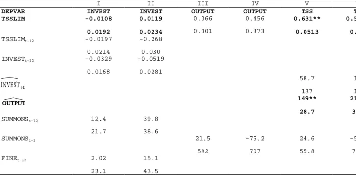
Tables 3A and 3B show that the coefficients on the emissions limits remain little different from their counterparts in Table 2: little of the correlation between limits and emissions is captured by our measures of firms investment and output responses. Nor is there any evidence that the investment responses had any effect on actual emissions. Finally, only for TSS do the firms output responses seem to have any impact on emissions (Table 3B).
The Full Model
The regressions reported in Tables 2 and 3 suggest that it is difficult to detect firms responses to environmental regulations through investment or modulation of output.
The importance of being able to distinguish between endogenous and exogenous UUUUUUU
legislation is paramount, as can be seen from two stylized examples. In the first, government legislation is set completely exogenously, that is, in response to whatever criteria the government deems appropriate without consulting the firms, and penalties are sufficiently credible that a representative firm pollutes at exactly the prescribed limit. The second case is the opposite of the firstthe legislation process is completely captured by firms, who cause limits to be set exactly in accordance with their production targets, and so of course subsequently observe these limits, and cause penalties to be light. An empirical observer would see a perfect correspondence between limits and emissions in both cases, and might erroneously conclude in the second that lowering the limits would cause a corresponding fall in emissions. But it is firms likely reaction to an exogenous change in legislation which we would like to estimate in the context of evaluating the effectiveness of the legislation in controlling firm behaviour. Columns V and VI of Tables 3A and 3B do describe, however, the same significant relationship between the limits themselves and emissions, these coefficients being as high as 0.4 for BOD and 0.6 for TSS. These correlations still pose a problem of inference. Do they represent firms controlling their emissions in response to exogenous changes in regulation imposed by government agencies? Or, less optimistically, do they represent regulatory capture: the tailoring of the limits to correspond to plants needs, after taking into account their capital investments and planning decisions?
The possibility of capture of a regulatory body by the agents that it is supposed to regulate is well known, but this possibility is not reflected in any of the analysis so far. Such capture is of course just an extreme example of the generic tendency for regulation not to be entirely exogenous to the phenomenon being regulated. Environmental limits are usually set following procedures of consultation with those being regulated, and therefore might be believed to respond not only to exogenous environmental factors (the costs and benefits of the pollution), but to existing constraints, lobbying, and so on. Figure 1, at the end of the text, which shows emissions and limits for a subset of the plants in the sample, is also suggestive of limits responding to past emissions or firmsrequirements: changes in limits often seem to follow changes in emissions rather than the opposite (see in particular Figure 1b). In equation form, we are particularly interested in the limits placed on emissions, and these may be said to be endogenous to the extent, if at all, that they are affected by firm actions (e.g., production) and characteristics (e.g., technology, capacity) and past pollution levels.UUUUUUU
An econometricians answer to the identification problem described here might be to look for instruments to generate an exogenous component of regulation. One could then examine whether firms behavior appeared responsive to this exogenous component.
What might such instruments look like? On one hand, we might consider as candidates attributes of the plants which affected the seriousness of the environmental threat posed by emissions into their water sources. These variables could reasonably be expected to affect government agencies regulatory decisions,
Actually, a Hausman test for the endogeneity of the limits (performed from UUUUUUUU
specifications III and VII in Table 2, using basins as an instrument) generated t-statistics of 6.5 and 5.0 for BOD and TSS respectively, so we can comfortably reject exogeneity of emission limits in the strict statistical sense implied by the use of this test.
but should not affect firms decisions regarding output or investment other than as responses to these decisions. Locational variables might constitute an example of such variables. Time dummies or trend terms might also be acceptable if we thought that the regulators view of the seriousness of emissions were evolving over time. On the other hand, we might consider attributes of the plants that were controlled by firms decisions, but only over the medium to long term. Plant capacity could be considered such an attribute. These variables may also affect the regulators decisions over limits, but would not be alterable by the firms quickly enough to be viewed as responses to regulation.UUUUUUUU
The third set of regressions performed for this paper are an attempt to implement the estimation strategy described in the previous paragraphs. First, the emissions limits themselves are regressed using ordinary least squares on a trend term interacted with dummy variables for the plants river basin location, and the trend term interacted with the plants capacities. These variables constitute the richest set of instruments we could generate from the data using the logic of the previous paragraph to define exogeneity. This first stage regression is reported in Table 4 for both BOD and TSS limits.
The second stage of the analysis is to relate firms decisions concerning investment and output to the predicted values from the first stage regressions, which we interpret as exogenous regulatory activity. These results are shown in columns I-IV of Tables 5A and 5B for BOD and TSS respectively. Columns I and II give our two specifications for the investment equation, relating firms reported abatement investments to exogenous limits, lagged limits, year lagged summons, fines, and enquiries, and capacity utilization (again a proxy for the business cycle).
For BOD, in the second specification there is a significant relationship between exogenous changes in the limit and reported investment and we interpret this as an interesting indication. Moreover, as in the simple specification of Table 3A, the hypothesis that the coefficients on the current and lagged limits sum to zero cannot be rejected at conventional significance levels. The magnitude of these coefficients is also similar to that in Table 3A. It seems likely that firms, then, are responding to changes in BOD limits by announcing abatement investments. There is, however, no evidence that the same is true for TSS limits (Table 5B, columns I and II).
Columns III and IV in Tables 5A and 5B give the results of the two specifications of the output equation. These equations are the counterparts of columns III and IV of Tables 3A and 3B, with the emissions limits replaced with instrumented values.
For BOD the coefficients in both specifications are significant only at the ten percent level. For TSS they are significant at all conventional levels. In all equations there is the increase in output following the imposition of a fine, described earlier. This could simply reflect firms relaxing more careful policies followed for the duration of the court case, but this can only be conjectured. The main interest lies in the change between Tables 3B and 5B for TSS: plants output does seem to be responsive to exogenous changes in emissions limits in Table 5B, whereas they were not responsive to the limits themselves in Table 3B. For TSS at least, the instrumental variables approach sheds new light on firms behavior.
As before, the question remains as to whether we can detect an effect on their actual emissions of firms responses to exogenous legislation. Columns V (VI) of Tables 5A and 5B report the regressions of emissions on the predicted values from columns I and III (II and IV), as well as the exogenous component of the limits, lagged emissions, and the other regulatory variables. For BOD (Table 5A) there is no evidence that the investment response reported in column II actually affects emissions at all. A first suggested explanation is that firms announce as abatement capital projects that might have been taken on for other reasons and that have only a secondary, perhaps negligible, impact on emissions. This suggestion is in part inspired from the aggregate picture the data paint (see Figure 2): emissions have not significantly decreased over the period studied. There are other reasons why firms may announce investments that do not generate discernible subsequent reductions in emissions: a second is that firms may be building emissions control equipment which has not yet come on line. We try to rule out this explanation by using a reasonably long lag of invest. Thirdly, there may also be expectations of future regulations, green advertizing, or other factors increasing the cost to firms of emissions.
For TSS (Table 5B), the hypothesis that the output modulation reported in columns III and IV does reduce emissions cannot be rejected at the ten percent level. Exogenous changes in TSS limits do seem to be affecting firms behavior enough to have a measurable impact on emissions.
Finally, in both the case of BOD and TSS, there is still a highly significant residual link between the instrumented limit and emissions, after accounting for the investment and output responses. The coefficient is of a magnitude of about 0.1 or 0.2 for BOD, and about 0.3 for TSS. This represents firms responding to the limits in ways undetected by our imperfect measurements of investment and output. This suggests that firms have ways of reducing emissions other than investing or modulating output: reallocating staff hours towards monitoring, better maintenance of pollution-control equipment or altering operational details within the plant. It is also noteworthy that the magnitude of the coefficients of the limit variables in the emissions equations are much lower than those reported in the naive regressions of Tables 2 and 3. This fact combined with the Hausman test (footnote 9) rejecting the exogeneity of the limits suggests that our approach through the full model was warranted.
4. Conclusions
Magat and Viscusi (1990) restrict attention to BOD emissions and suggest that firms reactions to TSS regulations may be similar. Our results suggest that this may not be the case. For BOD, firms seem to respond by announcing investments, but these investments do not seem to have much effect on emissions. This in turn suggests that policy may have placed undue emphasis on the abatement technology itself (see the first paragraph of the introduction) rather than its results. Portney (1990, page 5), in the context of United States environmental regulation, observed:
One finding is that much more attention has been devoted to ensuring that polluters get pollution equipment in place than to seeing that it is operated correctly.
In contrast, changes in TSS limits seem to affect firms short term output decisions, and the firms adjustments are reflected in lower emissions.
The overall impression that the results give, of a relative lack of impact on emissions, is reinforced by the graphs of industry wide aggregates and ratios shown in Figure 2. Between 1985 and 1989, BOD and TSS emissions per unit of output remained relatively flat, as did output itself. Aggregate limits fell slowly over this period, but exceeded emissions, which fluctuated but showed no strong downward trend.
Previous work has drawn attention to the fact that United States environmental penalties are more severe than those in Canada, and that this may explain the perceived differences in firms responses to legislation between the two countries. This lack of severity in Ontario may also explain the weakness of effect of the legislative variables used in this paper: emissions tend to increase after a fine is announced, for example. In particular, the lack of response of emissions to inquiries is in contrast with Magat and Viscusis (1990) results for the United States. The results in general are consonant with those in Lanoie and Laplante (1994), who use stock market data to suggest that expected penalties associated with environmental infractions in Canada are not sufficiently severe to have a significant impact on firm behavior. An alternative explanation is that many of the firms were in compliance by a sufficiently large margin that changes in limits would not be likely to modify their behavior: more than three-quarters of the observations in the sample were in compliance.
On a methodological level, this paper addresses empirical issues that previous work in the economics of environmental regulation has not. First, it is necessary to
distinguish between exogenous changes in regulations (roughly speaking, those following from considerations of social costs and benefits) and endogenous changes in regulations (roughly speaking, those following from firms past emissions or ability to abate). Second, it is possible to distinguish empirically between different modes of response on the part of firms. The data are imperfect, and the implementation of the empirical methodology can only be as successful as the data are accurate, but we hope that future work will be able to build on the methods used here. The ability to discern distinct firm responses to true regulator influence may in turn improve regulators ability to improve environmental business law.
References
Environment Canada. The Basic Technology of the Pulp and Paper Industry and its Environmental Protection Practices. Ottawa: Canada, 1983.
Fearnley, Joan. Impact de la réglementation des émissions de polluants dans les cours d'eau en Ontario pour l'industrie des pâtes et papiers. Mimeo. Montreal: Ecole des Hautes Etudes Commerciales, 1993.
Kmenta, Jan. Elements of Econometrics. Second Edition. London: Macmillan, 1986.
Lanoie, Paul, and Laplante, Benoît. The Market Response to Environmental Regulation in Canada: a Theoretical and Empirical Analysis. Southern Economic Journal 61 (January 1994): 659-673.
Laplante, Benoît, and Rilstone, Paul. Environmental Inspections and Emissions of the Pulp and Paper Industry in Quebec. Journal of Environmental Economics and Management 31, 1996: 19-37.
Magat, Wesley A. and Viscusi, W. Kip. Effectiveness of the EPA's Regulatory Enforcement: the Case of Industrial Effluent Standards. Journal of Law and Economics 33 (October 1990): 331-360.
Marin, E. Firm Incentives to Promote Technological Change in Pollution Control: Comment. Journal of Environmental Economics and Management 21 (1991): 297-300.
Milliman, Scott R., and Prince, Raymond. Firm Incentives to Promote Technological Change in Pollution Control. Journal of Environmental Economics and Management 17 (November 1989): 247-265.
Milliman, Scott R., and Prince, Raymond. Firm Incentives to Promote Technological Change in Pollution Control: Reply. Journal of Environmental Economics and Management 22 (May 1992): 292-296. Muoghalu, M., McRobison D., and Glascock J., Hazardous Waste Lawsuits,
Stockholder Returns and Deterrence, Southern Economic Journal, October 1990: 357-370.
Ontario Ministry of the Environment. Report on the Industrial Direct Discharges in Ontario. Toronto: Queen's Printer for Ontario, 1985-1989.
Ontario Ministry of the Environment. St. Clair River MISA Pilot Site Investigation, Volume II, Part I - Technical Summary. Toronto: Queen's Printer for Ontario, January 1991.
Portney, P. R. Public Policies for Environmental Protection. Washington DC: Resources for the Future, 1990.
Table 1 : Summary of Variables
Name Definition/Units Mean St. Dev. Source
BOD (emissions) kg/day over 30 days 11029 12180 Ontario Environment Min
TSS (emissions) kg/day over 30 days 3777 3165 Ontario Environment Min
BODlim kg/day over 30 days 18741 20417 Ontario Environment Min
TSSlim kg/day over 30 days 6002 4922 Ontario Environment Min
Invest Can. $ '000 p.a. 606 1179 Pulp and Paper Canada
Output m of water per month3 63104 58436 Ontario Environment Min
Summons 1 at 1st, 2 at 2nd... 0.551 1.047 Ontario Environment Min
Fine 1 at 1st, 2 at 2nd... 0.393 0.977 Ontario Environment Min
Inquiry 1 at 1st, 2 at 2nd... 4.401 6.998 Ontario Environment Min
Capa Tons/month 58339 130730 Pulp and Paper Canada
Utilisation Industry-wide Percent 0.957 0.014 Statistics Canada cat.
14-Basin1-5 Indicatora Ontario Environment Min
Region1-3 Indicatorb Ontario Environment Min
Season1-3 Indicatorc
Month1-11 Indicatord
Subind1-3 Indicatore Ontario Environment Min
Time Period of observation. 36.5 13.863
Notes : Default: Ottawa River, 1: Hudson Bay, 2: Lake Superior, 3: Lake Huron, 4: Lake Ontario, 5: St. Lawrencea
Default: Centre-west, 1: Northeast, 2: Northwest, 3: Southeast
b
Default: autumn (Sep-Oct-Nov), 1: winter (Dec-Jan-Feb), 2: spring (Mar-Apr-May), 3: summer (Jun-Jul-Aug)
c
Default: December
d
Default: Deinking/board/fine papers/tissue, 1: Kraft, 2: Sulphite-mechanical, 3: Corrugating
e
Report on Industrial Direct Discharges in Ontario (1985-89)
Table 2 :
POLLUTION EMISSIONS (BOD and TSS)
Coefficients/standard errors I II III IV V VI VII BODLIM 0.460** 0.230** 0.509** 0.295** 0.031 0.044 0.025 0.035 TSSLIM 0.645** 0.469** 0.533** 0.053 0.061 0.046 SUMMONSt-1 295** 418** 240 355* -151* -61.0 -176* -123 167 152 167 76.7 66.4 81.3 FINEt-1 171 317 186 341 -96.7 -76.3 -67.6 -131 181 164 186 83.2 73.1 89.5 INQUIRY -15.8 -5.21 13.593 29.537 8.97 5.54 4.71 14.3 21.2 19.97 22.87 6.89 5.68 7.61 BODt-12 0.203 0.033 0.200** 0.032 TSSt-12 0.050* 0. 0.024 0 CAPACITY 0.0226** 0.0171** 0.0077** 0. 0.0054 0.0058 0.0014 0 UTILIZATION 757 714 -1567 -3548 3874 1267 dummies basins T T T T regions T T T seasons T T T T months T T T subind T T T T T T T F 15.0 12.5 15.1 12.8 15.3 14.1 15.8 r-square 0.80 0.80 0.71 0.75 0.81 0.85 0.81 obs 720 720 720 720 720 720 72015
Table 3A :
REACTION EQUATIONS - BOD
Coefficients/standard errors
I II III IV V V
DEPVARa INVEST INVEST OUTPUT OUTPUT BOD B BODLIM -0.0129** -0.0137** 0.0214 0.283* 0.268** 0.4 0.0040 0.0047 0.1481 0.136 0.045 0. BODLIMt-12 0.0133** 0.0117 0.0051 0.0065 INVESTt-12 -0.0228 -0.0466 0.0141 0.0272 -170 42 252 1 -18.7 8 73.1 92 SUMMONSt-12 10.6 34.7 20.8 38.3 SUMMONSt-1 -186 -211 2 573 692 1 263* 115 FINEt-12 1.48 13.4 22.2 43.6
I II III IV V V 16 FINEt-1 936 159 1 604 130 1 1701* 745 INQUIRYt-12 1.42 6.04 3.90 8.28 INQUIRY 207** 268** -8.55 1 70.3 94.4 12.2 2 BODt-12 0.222** 0.1 0.032 0. CAPACITY 0.258** 0.224** 0.024 0.020 UTILIZATION -60.4 -197 9825 10212 146 657 11930 18410 dummies basins T T T regions T T seasons T T T months T T subind T T T T T F 14.0 13.1 21.0 18.1 13.8 13 r-square 0.05 0.06 0.94 0.86 0.84 0 obs 720 720 720 720 720 7
DEPVAR: Dependent variable
17
Table 3B :
REACTION EQUATIONS - TSS
Coefficients/standard errors
I II III IV V V
DEPVAR INVEST INVEST OUTPUT OUTPUT TSS T
TSSLIM -0.0108 0.0119 0.631** 0.5 0.0192 0.0234 0.0513 0. 0.366 0.456 0.301 0.373 TSSLIMt-12 -0.0197 -0.268 0.0214 0.030 INVESTt-12 -0.0329 -0.0519 0.0168 0.0281 58.7 1 137 1 149** 21 28.7 35 SUMMONSt-12 12.4 39.8 21.7 38.6 SUMMONSt-1 21.5 -75.2 24.6 -5 592 707 55.8 77 FINEt-12 2.02 15.1 23.1 43.5
I II III IV V V 18 FINEt-1 1029 -67.1 628 60.4 1702* -1 766 80 INQUIRYt-12 1.61 6.13 4.07 8.49 INQUIRY 187** 198* 3.19 -6 66.4 86.9 4.56 8 TSSt-12 0.0676** 0. 0.0243 0. CAPACITY 0.253** 0.245** 0.018 0.018 UTILIZATION -50.2 -174 10826 5896 144 652 12230 18300 dummies basins T T T regions T T seasons T T T months T T subind T T T T T F 11.7 12.3 17.9 16.2 14.4 15 r-square 0.04 0.05 0.93 0.87 0.88 0 obs 720 720 720 720 720 7
19
Table 4 :
First Stage Regression of Emissions Limits
BOD Std Error TSS Std Erro
PERIOD -339** 35.9 -77.7** 6.71 CAPA*BASIN1 4.62** 1.96 3.46** 0.442 CAPA*BASIN2 0.110** 0.003 0.0187** 0.0005 CAPA*BASIN3 -0.00972 0.0129 -0.0288** 0.0024 CAPA*BASIN4 0.0468** 0.0040 0.0180** 0.0008 CAPA*BASIN5 28.6** 7.23 29.6** 1.36 PERIOD*BASIN1 460** 66.9 50.8** 12.5 PERIOD*BASIN2 670** 32.7 125** 6.11 PERIOD*BASIN3 92.6** 39.3 226** 7.35 PERIOD*BASIN4 27.1 31.7 5.44 5.93 PERIOD*BASIN5 229** 87.7 77.7** 16.4 CONSTANT 15348** 914 3963** 171 r-square 0.86 0.92 obs 720 720
20
Table 5A :
REACTION EQUATIONS with ENDOGENOUS LIMITS - BOD
Coefficients/standard errors
I II III IV V V
DEPVAR INVEST INVEST OUTPUT OUTPUT BOD B -0.00254 0.00244 -0.0198** 0.155* 0.232* 0.0827** 0.2 0.0059 0.072 0.099 0.0252 0. BODLIMt-12 0.00336 0.00450 0.0166* 0.0078 INVESTt-12 -0.0244 -0.0440 0.0154 0.0282 -75.9 82 286 1 -100 67.1 24 98 SUMMONSt-12 10.8 29.7 22.4 40.0 SUMMONSt-1 247 -34.4 567 683 467** 63 146 1 FINEt-12 0.800 6.05 23.8 46.0
I II III IV V V 21 FINEt-1 1256* 1923** 418** 42 613 737 153 1 INQUIRYt-12 0.878 1.07 4.17 8.83 INQUIRY 133** 178* -5.74 67 47.7 70.5 23.9 18 BODt-12 0.280** 0.2 0.031 0. CAPACITY 0.242** 0.224** 0.019 0.019 UTILIZATION 23.5 -135 9656 4975 164 670 11690 17050 dummies basins T T T regions T T seasons T T T months T T subind T T T T T F 10.7 11.3 20.6 17.9 14.3 14 r-square 0.04 0.07 0.94 0.90 0.75 0 obs 720 720 720 720 720 7
22
Table 5B :
REACTION EQUATIONS with ENDOGENOUS LIMITS - TSS
Coefficients/standard errors
I II III IV V V
DEPVAR INVEST INVEST OUTPUT OUTPUT TSS T 0.00311 0.0260 0.00857 0.0238 0.816** 1.34** 0.301** 0.3 0.272 0.38 0.059 0. TSSLIMt-12 -0.0263 -0.0237 0.0188 0.0307 INVESTt-12 -0.0281 -0.0469 0.0158 0.0269 75.9 1 132 1 72.0* 99 32.2 41 SUMMONSt-12 12.4 42.8 20.7 37.0 SUMMONSt-1 238 -122 -99.4 -556 674 89.2 9 FINEt-12 2.30 18.5 22.0 42.2
I II III IV V V 23 FINEt-1 1369* 2013** -48.5 12 608 733 91.6 1 INQUIRYt-12 1.75 6.19 3.97 7.92 INQUIRY 151** 204** 0.187 -2 46.9 71.4 9.82 9 TSSt-12 0.0764** 0.07 0.0256 0.0 CAPACITY 0.245** 0.231** 0.018 0.016 UTILIZATION -81.5 69.7 8393 2868 136 698 11630 17540 dummies basins T T T regions T T seasons T T T months T T subind T T T T T F 10.1 11.2 22.4 19.0 15.6 15 r-square 0.04 0.06 0.94 0.90 0.57 0 obs 720 720 720 720 720 7
Vous pouvez consulter la liste complète des publications du CIRANO et les publications %
elles-mêmes sur notre site World Wide Web à l'adresse suivante : Liste des publications au CIRANO%%
Cahiers CIRANO / CIRANO Papers (ISSN 1198-8169)
96c-1 Peut-on créer des emplois en réglementant le temps de travail ? / par Robert Lacroix
95c-2 Anomalies de marché et sélection des titres au Canada / par Richard Guay, Jean-François L'Her et Jean-Marc Suret
95c-1 La réglementation incitative / par Marcel Boyer
94c-3 L'importance relative des gouvernements : causes, conséquences et organisations alternative / par Claude Montmarquette
94c-2 Commercial Bankruptcy and Financial Reorganization in Canada / par Jocelyn Martel
94c-1 Faire ou faire faire : La perspective de l'économie des organisations / par Michel Patry
Série Scientifique / Scientific Series (ISSN 1198-8177)
96s-24 Nonparametric Estimation of American Options Exercise Boundaries and Call Prices / Mark Broadie, Jérôme Detemple, Eric Ghysels, Olivier Torrès
96s-23 Asymmetry in Cournot Duopoly / Lars-Hendrik Röller, Bernard Sinclair-Desgagné
96s-22 Should We Abolish Chapter 11? Evidence from Canada / Timothy C.G. Fisher, Jocelyn Martel
96s-21 Environmental Auditing in Management Systems and Public Policy / Bernard Sinclair-Desgagné, H. Landis Gabel
96s-20 Arbitrage-Based Pricing When Volatility Is Stochastic / Peter Bossaert, Eric Ghysels, Christian Gouriéroux
96s-19 Kernel Autocorrelogram for Time Deformed Processes / Eric Ghysels, Christian Gouriéroux, Joanna Jasiak
96s-18 A Semi-Parametric Factor Model for Interest Rates / Eric Ghysels, Serena Ng 96s-17 Recent Advances in Numerical Methods for Pricing Derivative Securities /
Mark Broadie, Jérôme Detemple
96s-16 American Options on Dividend-Paying Assets / Mark Broadie, Jérôme Detemple
96s-15 Markov-Perfect Nash Equilibria in a Class of Resource Games / Gerhard Sorger 96s-14 Ex Ante Incentives and Ex Post Flexibility / Marcel Boyer et Jacques Robert 96s-13 Monitoring New Technological Developments in the Electricity Industry : An
International Perspective / Louis A. Lefebvre, Élisabeth Lefebvre et Lise Préfontaine
96s-12 Model Error in Contingent Claim Models Dynamic Evaluation / Eric Jacquier et Robert Jarrow