Sharp Bounds in the Binary Roy Model

Texte intégral

(1)2012s-06. Sharp Bounds in the Binary Roy Model Marc Henry, Ismael Mourifié. Série Scientifique Scientific Series. Montréal Février2012. © 2012 Marc Henry, Ismael Mourifié. Tous droits réservés. All rights reserved. Reproduction partielle permise avec citation du document source, incluant la notice ©. Short sections may be quoted without explicit permission, if full credit, including © notice, is given to the source..

(2) CIRANO Le CIRANO est un organisme sans but lucratif constitué en vertu de la Loi des compagnies du Québec. Le financement de son infrastructure et de ses activités de recherche provient des cotisations de ses organisations-membres, d’une subvention d’infrastructure du Ministère du Développement économique et régional et de la Recherche, de même que des subventions et mandats obtenus par ses équipes de recherche. CIRANO is a private non-profit organization incorporated under the Québec Companies Act. Its infrastructure and research activities are funded through fees paid by member organizations, an infrastructure grant from the Ministère du Développement économique et régional et de la Recherche, and grants and research mandates obtained by its research teams. Les partenaires du CIRANO Partenaire majeur Ministère du Développement économique, de l’Innovation et de l’Exportation Partenaires corporatifs Autorité des marchés financiers Banque de développement du Canada Banque du Canada Banque Laurentienne du Canada Banque Nationale du Canada Banque Royale du Canada Banque Scotia Bell Canada BMO Groupe financier Caisse de dépôt et placement du Québec CSST Fédération des caisses Desjardins du Québec Financière Sun Life, Québec Gaz Métro Hydro-Québec Industrie Canada Investissements PSP Ministère des Finances du Québec Power Corporation du Canada Rio Tinto Alcan State Street Global Advisors Transat A.T. Ville de Montréal Partenaires universitaires École Polytechnique de Montréal HEC Montréal McGill University Université Concordia Université de Montréal Université de Sherbrooke Université du Québec Université du Québec à Montréal Université Laval Le CIRANO collabore avec de nombreux centres et chaires de recherche universitaires dont on peut consulter la liste sur son site web. Les cahiers de la série scientifique (CS) visent à rendre accessibles des résultats de recherche effectuée au CIRANO afin de susciter échanges et commentaires. Ces cahiers sont écrits dans le style des publications scientifiques. Les idées et les opinions émises sont sous l’unique responsabilité des auteurs et ne représentent pas nécessairement les positions du CIRANO ou de ses partenaires. This paper presents research carried out at CIRANO and aims at encouraging discussion and comment. The observations and viewpoints expressed are the sole responsibility of the authors. They do not necessarily represent positions of CIRANO or its partners.. ISSN 1198-8177. Partenaire financier.

(3) Sharp Bounds in the Binary Roy Model. *. Marc Henry†, Ismael Mourifié ‡. Résumé / Abstract We derive the empirical content of an instrumental variables model of sectorial choice with binary outcomes. Assumptions on selection include the simple, extended and generalized Roy models. The derived bounds are nonparametric intersection bounds and are simple enough to lend themselves to existing inference methods. Identification implications of exclusion restrictions are also derived. Mots clés/key words : treatment effect, discrete outcomes, sectorial choice, partial. identification, intersection bounds. Codes JEL : C21, C25, C26. * The present version is of February 10, 2012. This research was supported by SSHRC Grant 410-2010-242 and was conducted in part, while Marc Henry was visiting the University of Tokyo and Ismael Mourifié was visiting Penn State. The authors thank their respective hosts for their hospitality and support. † Département de sciences économiques, Université de Montréal, C.P. 6128, succursale Centre-ville, Montréal Québec, H3C 3J7, Canada. Tel: 1 (514) 343-2404. Fax: 1 (514) 343-7221, email : marc.henry@umontreal. ‡ Université de Montréal..

(4) ´ MARC HENRY AND ISMAEL MOURIFIE. 2. Introduction A large literature has developed since Heckman and Honoré (1990) on the empirical content of the Roy model of sectorial choice with sector specific unobserved heterogeneity. Most of this literature, however, concerns the case of continuous outcomes and many applications, where outcomes are discrete, fall outside its scope. They include analysis of the effects of different training programs on the probability of renewed employment, of competing medical treatments or surgical procedures on the probability of survival, of higher education on the probability of migration and of competing policies on schooling decisions in developing countries among numerous others. The Roy model is still highly relevant to those applications, but very little is known of its empirical content in such cases. The case of discrete outcomes is considered in Chesher (2010) but the analysis doesn’t apply to binary outcomes. Sharp bounds are derived in binary outcome models with a binary endogenous regressor in Shaikh and Vytlacil (2011), Chiburis (2010), Jun, Pinkse, and Xu (2010) and Mourifié (2011) under a variety of assumptions, which all rule out sector specific unobserved heterogeneity. Finally, Heckman and Vytlacil (1999) derive identification conditions in a parametric version of the binary Roy model. We consider three distinct versions of the binary Roy model: the original model, where selection is based solely on the probability of success; the extended Roy model, where selection depends on the probability of success and a function of observable variables (sometimes called “nonpecuniary component”); and the generalized Roy model, with selection specific unobservable heterogeneity. When considering the generalized Roy model, we further distinguish restrictions on the selection equation and restrictions on the joint distribution of sector specific unobserved heterogeneity. We specifically consider the case, where selection variables are independent of sector specific unobserved heterogeneity and the case, where sector specific unobserved heterogeneity follows a factor structure proposed in Aakvik, Heckman, and Vytlacil (2005). Following Heckman, Smith, and Clements.

(5) DISCRETE ROY MODEL. 3. (1997), we apply results from optimal transportation theory to derive sharp bounds on the structural parameters, from which a range of treatment parameters can be derived. More specifically, we apply Theorem 1 of (Galichon and Henry 2011) (equivalently Theorem 3.2 of Beresteanu, Molchanov, and Molinari (2011)) to derive bounds for the generalized binary Roy model. The latter Theorem was recently applied in a similar context by Chesher, Rosen, and Smolinski (2011) to derive sharp bounds for instrumental variable models of discrete choice. We spell out the point identification implications of the bounds under certain exclusion restrictions. The bounds are simple enough to lend themselves to existing inferential methods, specifically Chernozhukov, Lee, and Rosen (2009) in the instrumental variables case. The remainder of the paper is organized as follows. Section 1 clarifies the analytical framework. In Section 2, sharp bounds are derived for the binary Roy model, when selection depends only on the probability of success and possibly on observable variables. Identification implications are spelled out under exclusion restrictions. Section 3 considers the generalized binary Roy model and the last section concludes.. 1. Analytical framework We adopt the framework of the potential outcomes model Y = Y1 D + Y0 (1 − D), where Y is an observed outcome, D is an observed selection indicator and Y1 , Y0 are unobserved potential outcomes. Heckman and Vytlacil (1999) trace the genealogy of this model and we refer to them for terminology and attribution. Potential outcomes are as follows: Yd = 1{Yd∗ > 0} = 1{F (d, Xd , ud ) > 0}, d = 1, 0,. (1.1). where 1{.} denotes the indicator function and F is an unknown function of the vector of observable random variables Xd and unobserved random variable ud . We make the following assumptions throughout the paper..

(6) ´ MARC HENRY AND ISMAEL MOURIFIE. 4. Assumption 1 (Weak separability). The functions F (d, Xd , ud ), d=1,0, both have weakly separable errors. As shown in Vytlacil (2002), potential outcomes can then be written Yd = 1{fd (Xd ) > ud } without loss of generality. Assumption 2 (Regularity). The sector specific unobserved variables ud , d = 1, 0, are uniformly continuous with respect to Lebesgue measure, so that they may be assumed without loss of generality to be distributed uniformly on [0, 1].. The normalization of Assumption 2 is very convenient, since it implies fd (xd ) = E(Yd |xd , z) and bounds on treatment effects parameters can be derived from bounds on the structural parameters f1 and f0 . Assumption 3 (Instruments). Observable variables Xd , d = 1, 0, and instruments Z are independent of (u1 , u0 ). Common components of X1 and X0 will be dropped from the notation in the remainder of the paper and by slight abuse of notation, Xd will refer only to the variables that are excluded from the equation for Y1−d and Z to variables that are excluded from both outcome equations (when the case arises).. As was the case in Aakvik, Heckman, and Vytlacil (2005), many of the results apply to the Tobit version of the model, where Yd = Yd∗ 1{Yd∗ > 0}, but for clarity of exposition, we only report results pertaining to the binary case.. 2. Sharp bounds for the binary Roy and extended Roy models 2.1. Simple binary Roy model. In the original model proposed by Roy (1951), the sector yielding the highest outcome is selected, i.e., D = 1{Y1∗ > Y0∗ }. In the binary case, this is equivalent to selecting the sector with the highest probability of success. The empirical content of the model under this selection rule is characterized in Figures 1 and 2..

(7) DISCRETE ROY MODEL. Figure 1.. 5. Characterization of the empirical content of the simple binary Roy model. in the unit square of the (u1 , u0 ) space. f1. 1 − f0 + f1. (Y = 0, D = 1). (Y = 1, D = 1). (Y = 0, D = 0) f0. f0. (Y = 1, D = 0). f0 − f1. f1. Figure 2.. Characterization of the empirical content of the simple binary Roy model. in the unit square of the (u1 , u0 ) space in case f0 = 0. f1. (Y = 0, D = 1) 1 − f1 (Y = 1, D = 1). (Y = 0, D = 0). f1.

(8) ´ MARC HENRY AND ISMAEL MOURIFIE. 6. For each value of the exogenous observable variables and each value of the pair (u1 , u0 ), the outcome is uniquely determined. If the joint distribution were known, the likelihood of each of the potential outcomes (Y = 1, D = 1), (Y = 1, D = 0), (Y = 0, D = 1) and (Y = 0, D = 0) would be determined. However, only the marginal distributions of u1 and u0 are fixed, not the copula, so that only the probability of vertical and horizontal bands in Figures 1 and 2 are uniquely determined. Thus we see for instance that f1 = P(Y = 1, D = 1) is identified when f0 = 0 (as in Figure 2) and f0 = P(Y = 1, D = 0) is identified when f1 = 0. But in other cases (as in Figure 1), we only know P(Y = 1, D = 1) ≤ f1 ≤ P(Y = 1) and P(Y = 1, D = 0) ≤ f0 ≤ P(Y = 1). The following proposition, proved in the Appendix, shows that these bounds are sharp. In all that follows, we shall use the notation P(i, j|X) for P(Y = i, D = j|X) and W = (Z, X1 , X0 ), ω = (z, x1 , x0 ).. Proposition 1 (Roy model). Under Assumptions 1-3, the following inequalities characterize the empirical content of the model.. sup P(1, 1|x1 , x0 , z) ≤ f1 (x1 ). h i ≤ inf P(1, 1|ω) + P(1, 0|ω)1{f0 (x0 ) > 0}. (2.1). sup P(1, 0|ω) ≤ f0 (x0 ). h i ≤ inf P(1, 0|ω) + P(1, 1|ω)1{f1 (x1 ) > 0}. (2.2). x0 ,z. x1 ,z. x0 ,z. x1 ,z. where the infima and suprema are taken over the domains of the excluded variables Z, X1 or X0 as indicated and when they exist.. Since the bounds in Proposition 1 are obtained as intersections over the domains of the excluded variables, they are called “intersection bounds”. They are also semiparametric in the non excluded variables. Inference on such bounds can be conducted with existing methods described in Chernozhukov, Lee, and Rosen (2009). A simple implication of selection equation D = 1{Y1∗ > Y0∗ } is that actual success is more likely than counterfactual success..

(9) DISCRETE ROY MODEL. 7. Assumption 4 (Roy model). E(Yd |D = d, Z, X1 , X0 ) ≥ E(Y1−d |D = d, Z, X1 , X0 ) for d = 1, 0.. Under Assumption 4, omitting conditioning variables for ease of notation, fd. =. E[Yd ]. =. E[Yd |D = d]P(D = d) + E[Yd |D = 1 − d]P(D = 1 − d). ≤. P[Y = 1, D = d] + E[Y1−d |D = 1 − d]P(D = 1 − d). =. P(Y = 1, D = d) + P(Y = 1, D = 1 − d).. Moreover, if fd > 0 and f1−d = 0, P(D = 1 − d) = 0. This implies that P(1, d|ω) ≤ E[Yd |ω] ≤ P(1, d|ω) + P(1, 1 − d|ω)1{E[Y1−d |ω] > 0} (with ω = (z, x1 , x0 )) characterizes the empirical content of the potential outcomes model Y = Y1 D + Y0 (1 − D) in all generality (i.e., without weak separability and without assumptions on the dimension of unobservable heterogeneity). It also shows that the simple binary Roy model has no empirical content beyond Assumption 4. Indeed, bounds (2.1) and (2.1) still hold under Assumptions 1-4. They are also sharp, since D = 1{Y1∗ > Y0∗ } implies Assumption 4. Therefore, the empirical content of the model defined by Assumption 4 is the same as the empirical content of the model defined by the selection equation D = 1{Y1∗ > Y0∗ }. Corollary 1. The empirical content of the model defined by Assumptions 1-4 is characterized by inequalities (2.1) and (2.2).. In case of exclusion restrictions, an immediate corollary to Proposition 1 gives conditions for identification of the outcome equations. Corollary 2 (Identification). Under Assumptions 1-4, the following hold (writing ω = (z, x1 , x0 ) as before)..

(10) ´ MARC HENRY AND ISMAEL MOURIFIE. 8. a. If there is x0 ∈ Dom(X0 ) such that f0 (x0 ) = 0, then f1 is identified over Dom(X1 ). b. If there is x1 ∈ Dom(X1 ) such that f1 (x1 ) = 0, then f0 is identified over Dom(X0 ). a’. Take x1 ∈ Dom(X1 ). If there is x0 ∈ Dom(X0 ) or z ∈ Dom(Z) such that P(1, 0|ω) = 0, then f1 (x1 ) is identified. b’. Take x0 ∈ Dom(X0 ). If there is x1 ∈ Dom(X1 ) or z ∈ Dom(Z) such that P(1, 1|ω) = 0, then f0 (x0 ) is identified.. The existence of valid instruments or exclusion restrictions is often problematic in applications of discrete choice models. However, in the Roy model of sectorial choice with sector specific unobserved heterogeneity, it is natural to expect some sector specific observed heterogeneity as well. Such sector specific observed heterogeneity would provide exclusion restrictions in the form of variables affecting outcome equation for Yd without affecting outcome equation for Y1−d . Such exclusion restrictions would yield intersection bounds in Proposition 1. Of course, even if it exists, sector specific observed heterogeneity may not satisfy a. or b. of Corollary 2. However, the availability of an exclusion restriction as in a. or b. of Corollary 2 is consistent with the spirit of a model of sector specific heterogeneity.. 2.2. Extended binary Roy model. Assumption 4 is very restrictive and recent research by Haultfoeuille and Maurel (2011) and Bayer, Khan, and Timmins (2011) on the Roy model with continuous outcomes has focused on an extended version, where selection depends on Y1∗ − Y0∗ and a function of observable variables g(Z, X1 , X0 ) sometimes called “non pecuniary component”. We now investigate the implications of this selection assumption in the binary case.. Assumption 5 (Observable heterogeneity in selection). D = 1{Y1∗ − Y0∗ > g(Z, X1 , X0 )} for some unknown function g of the vector of the observable variables Z, X1 and X0 ..

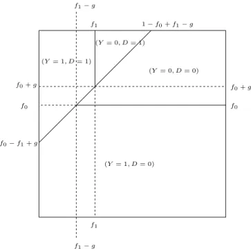
(11) DISCRETE ROY MODEL. 9. Under Assumptions 1-3 and 5, we may still characterize the empirical content of the model graphically, in Figures 3 and 4. We drop Z, X1 and X0 from the notation in the discussion below.. Figure 3.. Characterization of the empirical content of the extended binary Roy model. in the unit square of the (u1 , u0 ) space in case 0 ≤ g < f1 . f1. 1 − f0 + f1 − g. (Y = 0, D = 1). (Y = 1, D = 1). (Y = 0, D = 0). f0. f0. (Y = 1, D = 0) f0 − f1 + g. f1. For each value of (u1 , u0 ), the outcome is uniquely determined by f1 , f0 and g. Again, the missing piece to compute the likelihood of outcomes P(i, j), i, j = 1, 0, is the copula for (u1 , u0 ). From the knowledge of the probabilities of horizontal and vertical bands in the (u1 , u0 ) space, we can derive the sharp bounds on structural parameters f1 , f0 and g. Four cases are considered below to explain the bounds, which are derived formally and shown to be sharp in Proposition 2. a. Case where g ≥ f1 on Figure 4. The probability of outcome (Y = 1, D = 0) is seen to be exactly equal to the area of the lower horizontal band. Hence f0 = P(1, 0) is identified. Moreover, the area of the horizontal band (f0 , f0 − f1 + g) is smaller than the probability of outcome (Y = 1, D = 1). Hence g ≤ f1 + P(1, 1). Similar reasoning yields P(1, 1) ≤ f1 ≤ P(Y = 1) + P(0, 0)..

(12) ´ MARC HENRY AND ISMAEL MOURIFIE. 10. Figure 4.. Characterization of the empirical content of the extended binary Roy model. in the unit square of the (u1 , u0 ) space in case g ≥ f1 . f1. 1 − f0 + f1 − g (Y = 0, D = 1). (Y = 1, D = 1). (Y = 0, D = 0). f0 − f1 + g f0. f0 (Y = 1, D = 0). f1. b. Case where 0 ≤ g < f1 on Figure 3. The area of the lower horizontal band (0, f0 − f1 + g) is smaller than the probability of outcome (Y = 1, D = 0). Hence g ≤ f1 − f0 + P(1, 0). Moreover, the area of the horizontal band (0, f0 ) is larger than the probability of outcome (Y = 1, D = 0) and smaller than the probability of outcome (Y = 1). Hence P(1, 0) ≤ f0 ≤ P(Y = 1). Finally, P(1, 1) ≤ f1 ≤ P(Y = 1) + P(0, 0) still holds. c. Case where −f0 < g ≤ 0. Similarly to Case b., we obtain bounds g ≥ f1 − f0 + P(1, 1), P(1, 0) ≤ f0 ≤ P(Y = 1) + P(0, 1) and P(1, 1) ≤ f1 ≤ P(Y = 1). d. Case where g ≤ −f0 . Similarly to Case a., f1 = P(1, 1) is identified and P(1, 0) ≤ f0 ≤ P(Y = 1) + P(0, 1) and g ≥ −f0 − P(0, 1).. It is shown formally in Proposition 2 that the bounds discussed above hold and cannot be improved upon. The same arguments can be applied to derive the empirical content of the model where the.

(13) DISCRETE ROY MODEL. 11. selection equation generalizes Assumption 5 with D = 1{u0 > h(u1 , W )} and h strictly increasing in u1 , for all W . Assumption 5 is the special case, where h(u1 , W ) = u1 + f0 (X0 ) − f1 (X1 ) + g(W ). Proposition 2 (Sharp bounds for the extended binary Roy model). Under Assumptions 1-3 and 5, the empirical content of the model is characterized by the following (writing ω = (z, x1 , x0 ) as before). h supz,x0 P(1, 1|ω) ≤ f1 (x1 ) ≤ inf z,x0 P(1, 1|ω) + P(1, 0|ω)1{g(ω) > −f0 (x0 )} i +P(0, 0|ω)1{g(ω) > 0} , (2.3) h supz,x1 P(1, 0|ω) ≤ f0 (x0 ) ≤ inf z,x1 P(1, 0|ω) + P(1, 1|ω)1{g(ω) < f1 (x1 )} i +P(0, 1|ω)1{g(ω) < 0} and g(ω) ∈. h i h −f0 (x0 ) − P(0, 1|ω), −f0 (x0 ) ∪ f1 (x1 ) − f0 (x0 ) − P(1, 1|ω), i h i f1 (x1 ) − f0 (x0 ) + P(1, 0|ω) ∪ f1 (x1 ), f1 (x1 ) + P(0, 0|ω) ,. (2.4). where the infima and suprema are taken over the domain of Z, X1 or X0 as indicated and when they arise.. Simple identification conditions can be derived for f1 and f0 from the bounds of Proposition 2 under exclusion restrictions. However, it can be seen immediately that exclusion restrictions cannot identify g( ). Corollary 3 (Identification). Under Assumptions 1-3 and 5, the following hold (writing ω = (z, x1 , x0 ) as before). a. If there is z ∈ Dom(Z) and x0 ∈ Dom(X0 ) such that g(ω) ≤ −f0 (x0 ), then f1 (x1 ) = P(1, 1|ω) is identified. b. If there is z ∈ Dom(Z) and x1 ∈ Dom(X1 ) such that g(ω) ≥ f1 (x1 ), then f0 (x0 ) = P(1, 0|ω) is identified. a’. Take x1 ∈ Dom(X1 ). If there is x0 ∈ Dom(X0 ) or z ∈ Dom(Z) such that P(1, 0|ω) = P(0, 0|ω) = 0, then f1 (x1 ) is identified..

(14) ´ MARC HENRY AND ISMAEL MOURIFIE. 12. b’. Take x0 ∈ Dom(X0 ). If there is x1 ∈ Dom(X1 ) or z ∈ Dom(Z) such that P(1, 1|ω) = P(0, 1|ω) = 0, then f0 (x0 ) is identified.. As in the case of the simple Roy model, the sharp bounds of Proposition 2 take the form of intersection bounds and inference can be conducted with existing methods. When there are no instruments (or exclusion restrictions), however, the bounds are no longer intersection bounds. They become: P(1, 1) ≤ f1. ≤. P(1, 1) + P(1, 0)1{g > −f0 } + P(0, 0)1{g > 0},. P(1, 0) ≤ f0. ≤. P(1, 0) + P(1, 1)1{g < f1 } + P(0, 1)1{g < 0}. and g. ∈. h i h i h i −f0 − P(0, 1), −f0 ∪ f1 − f0 − P(1, 1), f1 − f0 + P(1, 0) ∪ f1 , f1 + P(0, 0) .. When the object of interest is treatment parameters only, the three dimensional identification region defined by the sharp bounds on (f1 , f0 , g) is projected on the two-dimensional space (f1 , f0 ). When there are no exclusion restrictions, this projection yields the Manski (2000) nonparametric bounds. If the object of interest is the non pecuniary component g, the three dimensional identification region is projected on the one-dimensional space for g into the single interval [−P(1, 1) − P(1, 0) − 2P(0, 1), P(1, 1) + P(1, 0) + 2P(0, 0)]. In the presence of instruments (or exclusion restrictions), the projections on (f1 , f0 ) and g can be much tighter and the projection on (f1 , f0 ) may even be reduced to a point, as in Corollary 3.. Testing for the presence of a non pecuniary component. As we have just seen, in the absence of exclusion restrictions, the projection of the identified region on the g space always contains zero, so that it is impossible to test the hypothesis g = 0. However, in the presence of exclusion restrictions, the hypothesis g = 0 may become testable. There is a non zero non pecuniary component in the selection equation if and only if the projection of the sharp bounds does not contain 0 or equivalently,.

(15) DISCRETE ROY MODEL. 13. if the hyperplane g = 0 does not intersect the three dimensional identification region for (f1 , f0 , g) defined by the sharp bounds in Proposition 2. It is also equivalent to the crossing of the intersection bounds in Proposition 1, in the sense that sup P(1, 1|x1 , x0 , z) x0 ,z. >. h i inf P(1, 1|ω) + P(1, 0|ω)1{f0 (x0 ) > 0}. x0 ,z. or sup P(1, 0|ω) > x1 ,z. h i inf P(1, 0|ω) + P(1, 1|ω)1{f1 (x1 ) > 0}. x1 ,z. so that by Proposition 1, the simple Roy model is rejected. In practice, the test for the existence of a non pecuniary component would be carried out by constructing a confidence region according to the methods proposed in Chernozhukov, Lee, and Rosen (2009) and checking, whether the hyperplane g = 0 intersects the confidence region. If it does, we fail to reject the hypothesis of existence of a non pecuniary component g and if it doesn’t, we reject the hypothesis at significance level equal to 1 minus the confidence level chosen for the confidence region. The hypotheses g ≥ 0 or g ≤ 0 may be tested in the same way.. 3. Sharp bounds for the generalized binary Roy model So far, we have assumed that selection occurs on the basis of success probability and other observable variables. We now turn to the general case, where unobservable heterogeneity, beyond u0 − u1 , may play a role in sectorial selection. Knowledge of (u1 , u0 ) now no longer uniquely determines the outcome (Y = i, D = j) as seen on Figure 5. Multiplicity of equilibria and lack of coherence of the model can be dealt with, however, with the optimal transportation approach of Galichon and Henry (2011), as shown in the proof of Theorem 1 below.. Theorem 1 (Sharp bounds for the generalized Roy model). Under Assumption 1-3, the empirical content of the model is characterized by inequalities (3.1)-(3.3) below (writing ω = (z, x1 , x0 ) as.

(16) ´ MARC HENRY AND ISMAEL MOURIFIE. 14. Figure 5.. Characterization of the empirical content of the generalized binary Roy. model in the unit square of the (u1 , u0 ) space. f1. (Y = 1, D = 1). (Y = 0, D = 1). or. or. (Y = 0, D = 0). (Y = 0, D = 0). f0. f0 (Y = 1, D = 0). (Y = 0, D = 1). or. or. (Y = 1, D = 1). (Y = 1, D = 0). f1. before). sup P(1, 1|ω). ≤ f1 (x1 ) ≤ 1 − sup P(0, 1|ω),. (3.1). sup P(1, 0|ω). ≤ f0 (x0 ) ≤ 1 − sup P(0, 0|ω). (3.2). z,x0. z,x1. z,x0. z,x1. and ³ ´ sup max 0, f0 (x0 ) − P(1, 0|ω) − P(0, 1|ω), f1 (x1 ) − P(1, 1|ω) − P(0, 0|ω) z. ≤ P(u1 ≤ f1 (x1 ), u0 ≤ f0 (x0 )|x1 , x0 ). (3.3). ³ ´ ≤ inf min P(Y = 1|ω), f1 (x1 ) + f0 (x0 ) − P(Y = 1|ω) . z. Theorem 1 is not an operational characterization of the empirical content of the model since the sharp bounds involve the unknown quantity P(u1 ≤ f1 (x1 ), u0 ≤ f0 (x0 )|x1 , x0 ), which, by the normalization of Assumption 2, is exactly the copula of (u1 , u0 ). In the case of total ignorance.

(17) DISCRETE ROY MODEL. 15. about the copula of (u1 , u0 ), after plugging Fréchet bounds max(f1 (x1 ) + f0 (x0 ) − 1, 0) ≤ P(u1 ≤ f1 (x1 ), u0 ≤ f0 (x0 )|x1 , x0 ) ≤ min(f1 (x1 ), f0 (x0 )), inequalities (3.3) are shown to be redundant. Hence we have the following.. Corollary 4. Sharp bounds for the generalized Roy model under Assumption 1-3 are given by inequalities (3.1) and (3.2).. In order to sharpen those bounds, we may consider restrictions on the copula for (u1 , u0 ) or restrictions on the selection equation. We consider both strategies in turn.. 3.1. Restrictions on selection. Consider the following selection model, where selection depends on Y1∗ − Y0∗ and g(Z, X1 , X0 ) and selection specific unobserved heterogeneity v, which is weakly separable and which is independent of (resp. dependent on) sector specific unobserved heterogeneity (u1 , u0 ) under Assumption 6 (resp. Assumption 7). As before, write W = (Z, X1 , X0 ).. Assumption 6. D = 1{Y1∗ − Y0∗ > g(W ) + v}, with v ⊥⊥ (u1 , u0 , W ) and Ev = 0 (without loss of generality).. With v ⊥ ⊥ (u1 , u0 ), we have P(ud ≤ g(z, x1 , x0 ) + v + f1 (x1 ) − f0 (x0 )|z, x1 , x0 ) = Ev E[1{ud ≤ g(z, x1 , x0 ) + v − f1 (x1 ) + f0 (x0 )}|z, x1 , x0 , v] = max(0, g(z, x1 , x0 ) − f1 (x1 ) + f0 (x0 )) and it is shown in Corollary 5 that the bounds on g( ) derived in Section 2 remain valid.. Corollary 5. Under assumptions 1-3 and 6, (2.4) holds.. As for the bounds on (f1 , f0 ), (2.3) remain valid under specific domain restrictions for v.. Assumption 7. D = 1{Y1∗ − Y0∗ > g(W ) + v}, with v ⊥⊥ W , Ev = 0 (without loss of generality)..

(18) ´ MARC HENRY AND ISMAEL MOURIFIE. 16. Note that Assumption 7 is equivalent to assuming the selection equation D = 1{h(W ) > η} with η arbitrarily dependant on (u1 , u0 ). Indeed, one can take h(W ) = f1 (X1 ) − f0 (X0 ) − g(W ) and η = v + u1 − u0 .. Corollary 6. Under Assumption 1-3 and 7, (3.1) and (3.2) are sharp bounds for f1 and f2 .. From Corollary 6, we conclude that the weak separability of the selection specific unobserved heterogeneity term has no empirical content, since the bounds are identical to the case, where there is no information on selection.. 3.2. Restrictions on the joint distribution of sector specific heterogeneity.. 3.2.1. Parametric restrictions on the copula. In case the copula for (u1 , u2 ) is parameterized with parameter vector θ, sharp bounds are obtained straightforwardly by replacing P(u1 ≤ f1 (x1 ), u0 ≤ f0 (x0 )|x1 , x0 ) with the parametric version F (f1 (x1 ), f0 (x0 ); θ) in (3.3).. 3.2.2. Perfect correlation. In the case of perfect correlation between the two sector specific unobserved heterogeneity variables, P(u1 ≤ f1 (x0 ), u0 ≤ f0 (x0 )) = min(f1 (x1 ), f0 (x0 )) so that the sharp bounds of Theorem 1 specialize to (3.1), (3.2), min(f1 (x1 ), f0 (x0 )) ≤ inf z P(Y = 1|z, x1 , x0 ) and supz P(Y = 1|z, x1 , x0 ) ≤ max(f1 (x1 ), f0 (x0 )), which are the bounds derived in Chiburis (2010). 3.2.3. Independence. In the special case, where the two sector specific errors are independent of each other u1 ⊥⊥ u0 , sharp bounds can be derived from Theorem 1 and P(u1 ≤ f1 (x0 ), u0 ≤ f0 (x0 )) = P(u1 ≤ f1 (x1 ))P(u0 ≤ f0 (x0 )) = f1 (x1 )f0 (x0 ).. 3.2.4. Factor structure. Theorem 1 also allows us to characterize the empirical content of the factor model for sector specific unobserved heterogeneity proposed in Aakvik, Heckman, and Vytlacil (2005)..

(19) DISCRETE ROY MODEL. 17. Assumption 8 (Factor model). Sector specific unobserved heterogeneity has factor structure ud = αd u + ηd , d = 1, 0, with Eu = 0, Eu2 = 1 (without loss of generality) and η1 ⊥⊥ η0 |u. ηd is uniformly distributed on [0, 1] for d = 1, 0, conditionally on u.. This factor specification for sector specific unobserved heterogeneity is particularly appealing in applications to the effects of employment programs. Success in securing a job depends on common unobservable heterogeneity in talent and motivation and sector specific noise. Under Assumptions 1, 3 and 8, we still have E[Yd |z, x1 , x0 ] = fd (xd ) and P(u1 ≤ f1 (x1 ), u0 ≤ f0 (x0 )|x1 , x0 ) =. Eu P(η1 ≤ f1 (x1 ) − α1 u, η0 ≤ f0 (x0 ) − α0 u|x1 , x0 , u). =. Eu P(η1 ≤ f1 (x1 ) − α1 u|x1 , u)P(η0 ≤ f0 (x0 ) − α0 u|x1 , x0 , u). =. f1 (x1 )f0 (x0 ) + α1 α0 .. Hence we can obtain sharp bounds on parameters f1 , f0 , α1 and α0 as follows. Corollary 7 (Sharp bounds for the factor model). Under Assumptions 1, 3 and 8, the empirical content of the model is characterized by (3.1), (3.2) and (writing ω = (z, x1 , x0 ) as before) ³ ´ sup max 0, f0 (x0 ) − P(1, 0|ω) − P(0, 1|ω), f1 (x1 ) − P(1, 1|ω) − P(0, 0|ω) z. ≤ f1 (x1 )f0 (x0 ) + α1 α0 ³ ´ ≤ inf min P(Y = 1|ω), f1 (x1 ) + f0 (x0 ) − P(Y = 1|ω) z. We recover the case of independent sector specific heterogeneity variables, when α1 = α0 = 0.. Conclusion We have derived sharp bounds in the simple, extended and generalized binary Roy models, including a factor specification proposed by Aakvik, Heckman, and Vytlacil (2005). The bounds are simple.

(20) ´ MARC HENRY AND ISMAEL MOURIFIE. 18. enough to lend themselves to existing inference methods for intersection bounds as in Chernozhukov, Lee, and Rosen (2009).. Appendix A. Proofs In all the proofs, we use the notation ω = (z, x1 , x0 ). When there is no ambiguity, we shall write f1 = f1 (x1 ), f0 = f0 (x0 ) and g = g(ω).. A.1. Proof of Proposition 1.. A.1.1. Validity of the bounds. See main text.. A.1.2. Sharpness of the bounds. To show that these bounds are sharp for f1 (x1 ) it is sufficient to construct joint distributions for (u∗0 , u∗1 ) such that f1 (x1 ) equals P (Y = 1, D = 1|ω) or P (Y = 1|ω) (and similarly for f0 (x0 )) and which is compatible with the observed data in the following sense:. (1) P (u∗0 ≤ f0 (x0 ), u∗1 ≥ u∗0 + f1 (x1 ) − f0 (x0 )|x1 , x0 ) = P (Y = 1, D = 0|ω), (2) P (u∗1 ≤ f1 (x1 ), u∗1 ≤ u∗0 + f1 (x1 ) − f0 (x0 )|x1 , x0 ) = P (Y = 1, D = 1|ω), (3) P (u∗0 ≥ f0 (x0 ), u∗1 ≥ u∗0 + f1 (x1 ) − f0 (x0 )|x1 , x0 ) = P (Y = 0, D = 0|ω), (4) P (u∗1 ≥ f1 (x1 ), u∗1 ≤ u∗0 + f1 (x1 ) − f0 (x0 )|x1 , x0 ) = P (Y = 0, D = 1|ω), (5) P (u∗0 ≤ f0 (x0 )|x0 ) ∈ [P (Y = 1, D = 0|ω), P (Y = 1|ω)]..

(21) DISCRETE ROY MODEL. 19. We assume in the following that f0 (x0 ) ≥ f1 (x1 ) (the opposite case can be treated similarly). Consider the following function f (u∗0 , u∗1 ) with values: 2P (Y =1,D=0|ω) 2f1 (x1 )f0 (x0 )−f1 (x1 )2. if. u∗1 ≤ f1 (x1 ), u∗1 ≥ u∗0 + f1 (x1 ) − f0 (x0 ),. 0. if. u∗1 ≥ f1 (x1 ), u∗0 ≤ f0 (x0 ),. 2P (Y =1,D=1|ω) (2−2f0 (x0 )+f1 (x1 ))f1 (x1 ). if. u∗1 ≤ f1 (x1 ), u∗1 ≤ u∗0 + f1 (x1 ) − f0 (x0 ),. 2P (Y =0,D=1|ω) (1−f0 (x0 ))2. if. u∗1 ≥ f1 (x1 ), u∗1 ≤ u∗0 + f1 (x1 ) − f0 (x0 ),. 2P (Y =0,D=0|ω) (1+f0 (x0 )−2f1 (x1 ))(1−f0 (x0 )). if. u∗0 ≥ f0 (x0 ), u∗1 ≥ u∗0 + f1 (x1 ) − f0 (x0 ).. It is easy to verify that this function is a density of a joint distribution which is compatible with the observed data (i.e respects conditions 1 to 5 above) and such as f1 (x1 ) = P (u∗1 ≤ f1 (x1 )|x1 ) = P (Y = 1|ω). This fact shows that P (Y = 1|ω) is the sharp upper bound for f1 (x1 ). Now, we will propose another joint distribution compatible with the observed data such that: f1 (x1 ) = P (u∗1 ≤ f1 (x1 )|x1 ) = P (Y = 1, D = 1|ω). Consider now the function f (u∗0 , u∗1 ) = with values: 0. if. u∗1 ≤ f1 (x1 ), u∗1 ≥ u∗0 + f1 (x1 ) − f0 (x0 ),. P (Y =1,D=0|ω) f0 (x0 )(1−f1 (x1 )). if. u∗1 ≥ f1 (x1 ), u∗0 ≤ f0 (x0 ),. 2P (Y =1,D=1|ω) (2−2f0 (x0 )+f1 (x1 ))f1 (x1 ). if. u∗1 ≤ f1 (x1 ), u∗1 ≤ u∗0 + f1 (x1 ) − f0 (x0 ),. 2P (Y =0,D=1|ω) (1−f0 (x0 ))2. if. u∗1 ≥ f1 (x1 ), u∗1 ≤ u∗0 + f1 (x1 ) − f0 (x0 ),. 2P (Y =0,D=0|ω) (1+f0 (x0 )−2f1 (x1 ))(1−f0 (x0 )). if. u∗0 ≥ f0 (x0 ), u∗1 ≥ u∗0 + f1 (x1 ) − f0 (x0 ).. It is also easy to verify that this function is a density of a joint distribution which is compatible with the observed data (i.e respects conditions 1 to 5) and such as f1 (x1 ) = P (u∗1 ≤ f1 (x1 )|x1 ) = P (Y = 1, D = 1|ω). This fact shows that P (Y = 1, D = 1|ω) is the sharp lower bound for f1 (x1 ). With the same strategy we can show that the bounds P (Y = 1, D = 0|ω) ≤ f0 (x0 ) ≤ P (Y = 1|ω) are sharp. This fact completes our Proof.. A.2. Proof of Proposition 2..

(22) ´ MARC HENRY AND ISMAEL MOURIFIE. 20. A.2.1. Validity of the bounds. To show validity of the bounds, we drop all the conditioning variables ω = (z, x1 , x0 ) from the notation. We have D = 1 ⇒ Y0∗ + g ≤ Y1∗ ⇒ 1{Y0∗ + g ≥ 0} ≤ 1{Y1∗ ≥ 0} ⇒ 1{Y0∗ + g ≥ 0}1{D = 1} ≤ 1{Y1∗ ≥ 0}1{D = 1} ⇒ E[1{Y0∗ + g ≥ 0}|D = 1] ≤ E[1{Y1∗ ≥ 0}|D = 1] ⇒ E[1{Y0∗ + g ≥ 0}|D = 1] ≤ E[Y1 |D = 1]. We can easily derive equivalent inequalities when D = 0. Hence, if D = 1{Y1∗ > Y0∗ + g} then E[1{Y0∗ + g ≥ 0}|D = 1] ≤ E[Y1 |D = 1] and E[Y1 |D = 0] ≤ E[1{Y0∗ + g ≥ 0}|D = 0]. Hence, when g ≥ 0, E[Y0 |D = 1] ≤ E[Y1 |D = 1] and when g ≤ 0, E[Y1 |D = 0] ≤ E[Y0 |D = 0]. Finally, if g = 0 we have E[Yd |D = d] ≥ E[Yd |D = 1 − d] where d ∈ {0, 1}. Those inequalities allow us to construct the sharp bounds for f1 and f0 in the case where D = 1{Y1∗ > Y0∗ + g}.Indeed, f1 = E[Y1 ] = E[Y1 , D = 1] + E[Y1 |D = 0]P (D = 0) and f0 = E[Y0 ] = E[Y0 , D = 0] + E[Y0 |D = 1]P (D = 1). Now, if g ≥ 0, then P (Y = 1, D = 1) ≤ f1 ≤ P (Y = 1, D = 1) + P (D = 0) and P (Y = 1, D = 0) ≤ f0 ≤ P (Y = 1). On the other hand, if g ≤ 0, P (Y = 1, D = 1) ≤ f1 ≤ P (Y = 1) and P (Y = 1, D = 0) ≤ f0 ≤ P (Y = 1, D = 0) + P (D = 1). Finally, f0 = E[1{u0 ≤ f0 }1{u1 ≥ u0 + f1 − f0 − g}] + E[1{u0 ≤ f0 }1{u1 ≤ u0 + f1 − f0 − g}]. Hence, if g ≥ f1 , then {u1 ≤ u0 + f1 − f0 − g} ⇒ {u0 ≥ f0 } and f0 (X0 ) ≤ E[1{u0 ≤ f0 }1{u1 ≥ u0 + f1 − f0 − g}] + E[1{u0 ≤ f0 }1{u0 ≥ f0 }] ≤ E[1{u0 ≤ f0 }1{u1 ≥ u0 + f1 − f0 − g}] = P (Y = 1, D = 0). Now the bounds for g can be obtained as follows.. • If g + f0 − f1 ≥ 0 and g ≤ f1 , then {u0 ≤ g + f0 − f1 } ⇒ {u0 ≤ u1 + g + f0 − f1 } and {u0 ≤ g +f0 −f1 } ⇒ {u0 ≤ f0 }. So {u0 ≤ g +f0 −f1 } ⇒ {u0 ≤ u1 +g +f0 −f1 }∩{u0 ≤ f0 }. Hence g + f0 − f1 = P (u0 ≤ g + f0 − f1 ) ≤ P ({u0 ≤ u1 + g + f0 − f1 } ∩ {u0 ≤ f0 }) = P (Y = 1, D = 0). • If g + f0 − f1 ≥ 0 and g ≥ f1 , then {u0 ≤ g + f0 − f1 } ⇒ {u0 ≤ u1 + g + f0 − f1 }, hence g + f0 − f1 = P (u0 ≤ g + f0 − f1 ) ≤ P ({u0 ≤ u1 + g + f0 − f1 }) = P (D = 0). As f0 = P (Y = 1, D = 0) we have g − f1 ≤ P (Y = 0, D = 0)..

(23) DISCRETE ROY MODEL. 21. • If g + f0 − f1 ≤ 0 and g ≥ −f0 , then by similar arguments, we have g + f0 − f1 ≥ −P (Y = 1, D = 1). • If g + f0 − f1 ≤ 0 and g ≤ −f0 , then g + f0 ≥ −P (Y = 0, D = 1).. A.2.2. Sharpness of the bounds. As previously our method consist in constructing joint distributions compatible with the observed data such that:. • if g(ω) > 0, f1 (x1 ) equals P (Y = 1, D = 1|ω) or P (Y = 1, D = 1|ω) + P (D = 0|ω), • if g(ω) < 0, f1 (x1 ) equals P (Y = 1, D = 1|ω) or P (Y = 1|ω),. and similarly for f0 (x0 ). The compatibility between the joint distribution and the observed data can be expressed as follows:. (1) P (u∗0 ≤ f0 (x0 ), u∗1 ≥ u∗0 + f1 (x1 ) − f0 (x0 ) − g(ω)|ω) = P (Y = 1, D = 0|ω), (2) P (u∗1 ≤ f1 (x1 ), u∗1 ≤ u∗0 + f1 (x1 ) − f0 (x0 ) − g(ω)|ω) = P (Y = 1, D = 1|ω), (3) P (u∗0 ≥ f0 (x0 ), u∗1 ≥ u∗0 + f1 (x1 ) − f0 (x0 ) − g(ω)|ω) = P (Y = 0, D = 0|ω), (4) P (u∗1 ≥ f1 (x1 ), u∗1 ≤ u∗0 + f1 (x1 ) − f0 (x0 ) − g(ω)|ω) = P (Y = 0, D = 1|ω), (5). (a) if g > 0, P (u∗0 ≤ f0 (x0 )|x0 ) ∈ [P (Y = 1, D = 0|ω), P (Y = 1|ω)], (b) if g < 0, P (u∗0 ≤ f0 (x0 )|x0 ) ∈ [P (Y = 1, D = 0|ω), P (Y = 1, D = 0|ω) + P (D = 1|ω)].. Assume that f0 (x0 ) > f1 (x1 ), 0 < g(ω) < f1 (x1 ) and f0 (x0 ) + g(ω) < 1 as in Figure 6. Other cases.

(24) ´ MARC HENRY AND ISMAEL MOURIFIE. 22. Figure 6.. Characterization of the empirical content of the extended binary Roy model. in the unit square of the (u1 , u0 ) space in case f0 (x0 ) > f1 (x1 ), 0 < g(ω) < f1 (x1 ) and f0 (x0 ) + g(ω) < 1. f1 − g f1. 1 − f0 + f1 − g. (Y = 0, D = 1) (Y = 1, D = 1) (Y = 0, D = 0) f0 + g. f0 + g. f0. f0. f0 − f1 + g (Y = 1, D = 0). f1 f1 − g. can be treated similarly. Consider the function f (u∗0 , u∗1 ) with values:. 0. if. u∗0 ≤ g(ω) + f0 (x0 ) − f1 (x1 ), u∗1 ≥ f1 (x1 ),. P (Y =1,D=0|ω) f1 (x1 )(g(ω)+f0 (x0 )−f1 (x1 )). if. u∗0 ≤ g(ω) + f0 (x0 ) − f1 (x1 ), u∗1 ≤ f1 (x1 ),. 0. if. u∗0 ≥ g(ω) + f0 (x0 ) − f1 (x1 ), u∗0 ≤ f0 (x0 ) and u∗1 ≤ u∗0 + f1 (x1 ) − f0 (x0 ) − g(ω),. 2P (Y =0,D=0|ω) g(ω)g(ω). if. u∗0 ≥ f0 (x0 ), u∗1 ≤ f1 (x1 ), u∗1 ≥ u∗0 + f1 (x1 ) − f0 (x0 ) − g(ω),. 0. if. u∗0 ≥ f0 (x0 ), u∗1 ≥ f1 (x1 ), u∗1 ≥ u∗0 + f1 (x1 ) − f0 (x0 ) − g(ω),. 2P (Y =1,D=1|ω) (2−2(f0 (x0 )+g(ω))+f1 (x1 ))f1 (x1 ). if. u∗1 ≤ f1 (x1 ), u∗1 ≤ u∗0 + f1 (x1 ) − f0 (x0 ) − g(ω),. 2P (Y =0,D=1|ω) (1−f0 (x0 )−g(ω))2. if. u∗1 ≤ f1 (x1 ), u∗1 ≤ u∗0 + f1 (x1 ) − f0 (x0 ) − g(ω)..

(25) DISCRETE ROY MODEL. 23. It is easy to verify that this function is a density of a joint distribution which is compatible with the observed data (i.e respects conditions 1 to 5a) and such that f1 (x1 ) = P (u∗1 ≤ f1 (x1 )|x1 ) = P (Y = 1, D = 1|ω) + P (D = 0|ω) and g(ω) + f0 (x0 ) − f1 (x1 ) = P (u∗0 ≤ g(ω) + f0 (x0 ) − f1 (x1 )|ω) = P (Y = 1, D = 0|ω). In the previous section, we showed that P (Y = 1, D = 0|ω) is an upper bound for g(ω) + f0 (x) − f1 (x) in case g(ω) < f1 (x1 ). Here we construct a joint distribution which hits this upper bound. This fact shows that P (Y = 1, D = 1|ω) + P (D = 0|ω) is the sharp upper bound for f1 (x1 ) and that P (Y = 1, D = 0|ω) is the sharp upper bound for g(ω) + f0 (x) − f1 (x). We now propose a joint distribution such that f1 (x1 ) = P (u∗1 ≤ f1 (x1 )|x1 ) = P (Y = 1, D = 1|ω) and g(ω) + f0 (x0 ) − f1 (x1 ) = P (u∗0 ≤ g(ω) + f0 (x0 ) − f1 (x1 )|ω) = P (Y = 1, D = 0|ω). Consider the function f (u∗0 , u∗1 ) with values:. P (Y =1,D=0|ω) (1−f1 (x1 ))(g(ω)+f0 (x0 )−f1 (x1 )). if. u∗0 ≤ g(ω) + f0 (x0 ) − f1 (x1 ), u∗1 ≥ f1 (x1 ),. 0. if. u∗0 ≤ g(ω) + f0 (x0 ) − f1 (x1 ), u∗1 ≤ f1 (x1 ),. 0. if. u∗0 ≥ g(ω) + f0 (x0 ) − f1 (x1 ), u∗0 ≤ f0 (x0 ) and u∗1 ≤ u∗0 + f1 (x1 ) − f0 (x0 ) − g(ω),. 0. if. u∗0 ≥ f0 (x0 ), u∗1 ≤ f1 (x1 ) and u∗1 ≥ u∗0 + f1 (x1 ) − f0 (x0 ) − g(ω),. P (Y =0,D=0|ω) (1−f1 (x1 ))(1−f0 (x0 ))− 12 (1−f0 (x0 )−g(ω))2. if. u∗0 ≥ f0 (x0 ), u∗1 ≥ f1 (x1 ) and u∗1 ≥ u∗0 + f1 (x1 ) − f0 (x0 ) − g(ω),. 2P (Y =1,D=1|ω) (2−2(f0 (x0 )+g(ω))+f1 (x1 ))f1 (x1 ). if. u∗1 ≤ f1 (x1 ), u∗1 ≤ u∗0 + f1 (x1 ) − f0 (x0 ) − g(ω),. 2P (Y =0,D=1|ω) (1−f0 (x0 )−g(ω))2. if. u∗1 ≥ f1 (x1 ), u∗1 ≤ u∗0 + f1 (x1 ) − f0 (x0 ) − g(ω).. It is also easy to verify that this function is a density of a joint distribution which is compatible with the observed data (i.e respects conditions 1 to 5a) and such that f1 (x1 ) = P (u∗1 ≤ f1 (x1 )|x1 ) = P (Y = 1, D = 1|ω) and g(ω) + f0 (x0 ) − f1 (x1 ) = P (u∗0 ≤ g(ω) + f0 (x0 ) − f1 (x1 )|ω) = P (Y = 1, D = 0|ω). This fact shows that P (Y = 1, D = 1|ω) is the sharp lower bound for f1 (x1 ). With the same.

(26) ´ MARC HENRY AND ISMAEL MOURIFIE. 24. strategy we can show that P (Y = 1, D = 0|ω) ≤ f0 (x0 ) ≤ P (Y = 1|ω)] is sharp. This fact completes our Proof.. A.3. Proof of Theorem 1. Under Assumptions 1-3, the model can be equivalently written (Y, D) ∈ G((u1 , u0 )|W ) almost surely conditionally on W = (Z, X1 , X0 ), where G is a multi-valued mapping, which to (u1 , u0 ) associates (y, d) = G((u1 , u0 )|W ) = {(1, 1), (1, 0)} if u1 ≤ f1 (x1 ) and u0 ≤ f0 (x0 ), {(0, 1), (1, 0)} if u1 > f1 (x1 ) and u0 ≤ f0 (x0 ), {(1, 1), (0, 0)} if u1 ≤ f1 (x1 ) and u0 > f0 (x0 ) and {(0, 1), (0, 0)} if u1 > f1 (x1 ) and u0 > f0 (x0 ). Hence Theorem 1 of Galichon and Henry (2011) applies and the empirical content of the model is characterized by the collection of inequalities P (A|W ) ≤ P ((u1 , u0 ) : G((u1 , u0 )|W ) hits A|W ) for each subset A of {(0, 0), (0, 1), (1, 0), (1, 1)} (i.e., 16 inequalities). The only non redundant inequalities are P (1, 1|W ) ≤ f1 (X1 ), P (1, 0|W ) ≤ f0 (X0 ), P (0, 1|W ) ≤ 1 − f1 (X1 ), P (0, 0|W ) ≤ 1 − f0 (X0 ), P (Y = 0|W ) ≤ 1 − P (u1 ≤ f1 (X1 ), u0 ≤ f0 (X0 )|X1 , X0 ), P (Y = 1|W ) ≤ 1 − P (u1 > f1 (X1 ), u0 > f0 (X0 )|X1 , X0 ), P (0, 0|W ) + P (1, 1|W ) ≤ P (u1 ≤ f1 (X1 ), u0 ≤ f0 (X0 )|X1 , X0 ) + P (u0 > f0 (X0 )|X0 ) and P (0, 1|W ) + P (1, 0|W ) ≤ P (u1 ≤ f1 (X1 ), u0 ≤ f0 (X0 )|X1 , X0 ) + P (u1 > f1 (X1 )|X1 ). After some manipulation, the result follows.. A.4. Proof of Corollary 5. We show that the bounds (2.4) for g remain valid. We drop conditioning variables from the notation throughout this section.. • If g +v +f0 −f1 ≥ 0 and g +v ≤ f1 , then {u0 ≤ g +v +f0 −f1 } ⇒ {u0 ≤ u1 +g +v +f0 −f1 } and {u0 ≤ g + v + f0 − f1 } ⇒ {u0 ≤ f0 }. So {u0 ≤ g + v + f0 − f1 } ⇒ {u0 ≤ u1 + g + v + f0 − f1 } ∩ {u0 ≤ f0 }. Therefore P (u0 − v ≤ g + f0 − f1 ) ≤ P ({u0 ≤ u1 + g + v + f0 − f1 } ∩ {u0 ≤ f0 }) = P (Y = 1, D = 0). • If g +v +f0 −f1 ≥ 0 and g +v ≥ f1 , then {u0 ≤ g +v +f0 −f1 } ⇒ {u0 ≤ u1 +g +v +f0 −f1 }. Therefore P (u0 − v ≤ g + f0 − f1 ) ≤ P ({u0 ≤ u1 + g + v + f0 − f1 }) = P (D = 0)..

(27) DISCRETE ROY MODEL. 25. • If g+v+f0 −f1 ≤ 0 and g+v ≥ −f0 , then {u1 ≤ f1 −f0 −g−v} ⇒ {u1 ≤ u0 +f1 −f0 −g−v} and {u1 ≤ f1 − f0 − g − v} ⇒ {u1 ≤ f1 }. So {u1 ≤ f1 − f0 − g − v} ⇒ {u1 ≤ u0 + f1 − f0 − g −v}∩{u1 ≤ f1 }. Therefore P (u1 +v ≤ f1 −f0 −g) ≤ P ({u1 ≤ u0 +f1 −f0 −g −v}∩{u1 ≤ f1 }) = P (Y = 1, D = 1). • If g+v+f0 −f1 ≤ 0 and g+v ≤ −f0 , then {u1 ≤ f1 −f0 −g−v} ⇒ {u1 ≤ u0 +f1 −f0 −g−v}. Hence P (u1 + v ≤ f1 − f0 − g) ≤ P (u1 ≤ u0 + f1 − f0 − g − v) = P (D = 1). Now, since v ⊥⊥ (u0 , u1 ), we have: P (u0 ≤ g + v + f0 − f1 ) = Ev [E[1{u0 ≤ g + v + f0 − f1 }|v]] = Ev [g + v + f0 − f1 ] = g + f0 − f1 . Then, we get the following: • If g + v + f0 − f1 ≥ 0 and g + v ≤ f1 , then g + f0 − f1 ≤ P (Y = 1, D = 0). • If g + v + f0 − f1 ≥ 0 and g + v ≥ f1 , then g − f1 ≤ P (Y = 0, D = 0). • If g + v + f0 − f1 ≤ 0 and g + v ≥ −f0 , then g + f0 − f1 ≥ −P (Y = 1, D = 1). • If g + v + f0 − f1 ≤ 0 and g + v ≤ −f0 , then g + f0 ≥ −P (Y = 0, D = 1). which completes the proof.. A.5. Proof of Corollary 6. Our goal here is to show that the following bounds are sharp for f0 and f1 . P (Y = 1, D = 1|ω). ≤ f1 (x1 ) ≤ P (Y = 1, D = 1|ω) + P (D = 0|ω). P (Y = 1, D = 0 | ω). ≤ f0 (x0 ) ≤ P (Y = 1, D = 0|ω) + P (D = 1|ω).. The previous results show that the lower bounds are sharp. Now, to show that these bounds are sharp for f1 (x1 ) it is sufficient to construct a joint distribution (u∗0 , u∗1 ) such that f1 (x1 ) equals P (Y = 1, D = 1|ω) + P (D = 0|ω) and f (0, x) = P (Y = 1, D = 0|ω) + P (D = 1|ω) and which is compatible with the observed data in the following sense: (1) P (u∗0 ≤ f0 (x0 ), u∗1 ≥ u∗0 + f1 (x1 ) − f0 (x0 ) − g(ω) − v|ω) = P (Y = 1, D = 0|ω).

(28) ´ MARC HENRY AND ISMAEL MOURIFIE. 26. (2) P (u∗1 ≤ f1 (x1 ), u∗1 ≤ u∗0 + f1 (x1 ) − f0 (x0 ) − g(ω) − v|ω) = P (Y = 1, D = 1|ω) (3) P (u∗0 ≥ f0 (x0 ), u∗1 ≥ u∗0 + f1 (x1 ) − f0 (x0 ) − g(ω) − v|ω) = P (Y = 0, D = 0|ω) (4) P (u∗1 ≥ f1 (x1 ), u∗1 ≤ u∗0 + f1 (x1 ) − f0 (x0 ) − g(ω) − v|ω) = P (Y = 0, D = 1|ω) Define the following joint distribution (u∗0 , u∗1 , v ∗ ) such that u∗0 + u∗1 ≤ f1 (x1 ) + f0 (x0 ) and 2v ∗ = 3u∗0 − 3u∗1 − 3f0 (x0 ) + 3f1 (x1 ) − 2g(ω). Under the condition that u∗0 + u∗1 ≤ f1 (x1 ) + f0 (x0 ), we have {u∗1 ≥ u∗0 +f1 (x1 )−f0 (x0 )−g(ω)−v ∗ } ⇒ {u∗1 ≤ f1 (x1 )} and {u∗1 ≤ u∗0 +f1 (x1 )−f0 (x0 )−g(ω)−v ∗ } ⇒ {u∗0 ≤ f0 (x0 )}. Hence, f1 (x1 ) = P (u∗1 ≤ f1 (x1 ), u∗1 ≤ u∗0 + f1 (x1 ) − f0 (x0 ) − g(ω) − v|ω) +P (u∗1 ≤ f1 (x1 ), u∗1 ≥ u∗0 + f1 (x1 ) − f0 (x0 ) − g(ω) − v|ω) = P (u∗1 ≤ f1 (x1 ), u∗1 ≤ u∗0 + f1 (x1 ) − f0 (x0 ) − g(ω) − v|ω) +P (u∗1 ≥ u∗0 + f1 (x1 ) − f0 (x0 ) − g(ω) − v|ω) = P (Y = 1, D = 1|ω) + P (D = 0|ω). With the same strategy, we can also show f0 (x0 ) = P (Y = 1, D = 0|ω) + P (D = 1|ω).. References Aakvik, A., J. Heckman, and E. Vytlacil (2005): “Estimating treatment effects for discrete outcomes when responses to treatment vary: an application to Norwegian vocational rehabilitation programs,” Journal of Econometrics, 125, 15–51. Bayer, P., S. Khan, and C. Timmins (2011): “Nonparametric identification and estimation in a Roy model with common nonpecuniary returns,” Journal of Business and Economic Statistics, 29, 201–215. Beresteanu, A., I. Molchanov, and F. Molinari (2011): “Sharp identification regions in models with convex predictions,” Econometrica, 79, 1785–1821..

(29) DISCRETE ROY MODEL. 27. Chernozhukov, V., S. Lee, and A. Rosen (2009): “Inference on intersection bounds,” CEMMAP Working Paper CWP19/09. Chesher, A. (2010): “Instrumental variable models for discrete outcomes,” Econometrica, 78, 575–601. Chesher, A., A. Rosen, and K. Smolinski (2011): “An instrumental variable model of multiple discrete choice,” CEMMAP Working Paper CWP06/11. Chiburis, R. (2010): “Semiparametric bounds on treatment effect,” Journal of Econometrics, 159, 267–275. Galichon, A., and M. Henry (2011): “Set identification in models with multiple equilibria,” Review of Economic Studies, 78, 1264–1298. Haultfoeuille, X., and A. Maurel (2011): “Inference on an extended Roy model, with an application to schooling decisions in France,” unpublished manuscript. ´ (1990): “The empirical content of the Roy model,” Econometrica, Heckman, J., and B. Honore 58, 1121–1149. Heckman, J., J. Smith, and N. Clements (1997): “Making the most out of programme evaluation and social experiments: accounting for heterogeneity in programme impacts,” Review of Economic Studies, 64, 487–535. Heckman, J., and E. Vytlacil (1999): “Local instrumental variables and latent variable models for identifying and bounding treatment effects,” Proceedings of the National Academy of Sciences, 96, 4730–4734. Jun, S., J. Pinkse, and H. Xu (2010): “Tighter bounds in triangular systems,” Journal of Econometrics, 161, 122–128. Manski, C. (2000): “Nonparametric bounds on treatment effects,” American Economic Review, Papers and Proceedings, 80, 319–323..

(30) 28. ´ MARC HENRY AND ISMAEL MOURIFIE. ´, I. (2011): “Sharp bounds on treatment effects,” unpublished manuscript. Mourifie Roy, A. (1951): “Some thoughts on the distribution of earnings,” Oxford Economic Papers, 3, 135–146. Shaikh, A., and E. Vytlacil (2011): “Partial identification in triangular systems of equations with binary dependent variables,” Econometrica, 79, 949–955. Vytlacil, E. (2002): “Independence, monotonicity and latent index models: an equivalence result,” Econometrica, 70, 331–341..

(31)