HAL Id: hal-01828724
https://hal.archives-ouvertes.fr/hal-01828724
Submitted on 3 Jul 2018
HAL is a multi-disciplinary open access
archive for the deposit and dissemination of
sci-entific research documents, whether they are
pub-lished or not. The documents may come from
teaching and research institutions in France or
abroad, or from public or private research centers.
L’archive ouverte pluridisciplinaire HAL, est
destinée au dépôt et à la diffusion de documents
scientifiques de niveau recherche, publiés ou non,
émanant des établissements d’enseignement et de
recherche français ou étrangers, des laboratoires
publics ou privés.
Operational Modal Analysis in Frequency Domain using
Gaussian Mixture Models
Ankit Chiplunkar, Joseph Morlier
To cite this version:
Ankit Chiplunkar, Joseph Morlier. Operational Modal Analysis in Frequency Domain using Gaussian
Mixture Models. The 35th International Modal Analysis Conference (IMAC XXXV), Jan 2017, Los
Angeles, United States. pp.47-53. �hal-01828724�
Operational Modal Analysis in Frequency Domain using Gaussian Mixture
Models
Ankit Chiplunkar
∗Airbus Operations S.A.S., Toulouse, 31060, France
Joseph Morlier
†Universit ´e de Toulouse, CNRS, ISAE-SUPAERO, Institut Cl ´ement Ader (ICA), Toulouse, 31077, France
ABSTRACT
Operational Modal Analysis is widely gaining popularity as a means to perform system identification of a structure. Instead of using a detailed experimental setup Operational Modal Analysis relies on measurement of ambient displacements to identify the system. Due to the random nature of ambient ex-citations and their output responses, various statistical meth-ods have been developed throughout the literature both in the time-domain and the frequency-domain. The most popular of these algorithms rely on the assumption that the structure can be modelled as a multi degree of freedom second order differential system. In this paper we drop the second order differential assumption and treat the identification problem as a curve-fitting problem, by fitting a Gaussian Mixture Model in the frequency domain. We further derive equivalent mod-els for the covariance-driven and the data-driven algorithms. Moreover, we introduce a model comparison criterion to au-tomatically choose the optimum number of Gaussian’s. Later the algorithm is used to predict modal frequencies on a simu-lated problem.
NOMENCLATURE [M ] Mass Matrix [C] Damping Matrix [K] Stiffness Matrix
{x(t)} Displacement vector at time t {f (t)} Force vector at time t
k(τ ) Auto-correlation function at time-lag τ S(s) Spectral Density at s
GP Gaussian Process Q Number Of Gaussian’s GM M Gaussian Mixture Model OM A Operational Modal Analysis BIC Bayesian Information Criterion M LE Maximum Likelihood Estimate
k Number Of free parameters in an algorithm
∗PhD Candidate, Flight Physics Airbus Operations, 316 route de
Bayonne 31060
†Professor, Universit´e de Toulouse, CNRS, ISAE-SUPAERO,
Insti-tut Cl´ement Ader (ICA), 10 avenue Edouard Belin 31077 TOULOUSE Cedex 4
1 INTRODUCTION
Modal analysis has been widely used as a means of identify-ing dynamic properties such as modal frequencies, dampidentify-ing ratios and mode shapes of a structural system. Traditionally, the system is subjected to artificial input excitations and output deformations (displacements, velocities or accelerations) are measured. These later help in identifying the modal parame-ters of the system, this process is called Experimental Modal Analysis (EMA). In the last few decades several algorithms pri-marily using the assumption of second order differential, Multi Degree Of Freedom (MDOF) system (equation 1) have been developed to find modal parameters in EMA[1] [2].
[M ]{¨x(t)} + [C]{ ˙x(t)} + [K]{x(t)} = {f (t)} (1)
Here, [M ], [C] and [K] denote the mass, damping and stiff-ness matrices respectively. While, {x(t)} and {f (t)} denote the displacement and force vectors at the time t.
Since the last decade Operational Modal Analysis (OMA) has gained considerable interest in the community. OMA identi-fies the modal parameters only from the output measurements while assuming ambient excitations as random noise. OMA is cheaper because it does not require expensive experimental setup and and can be used in real time operational use cases such as health monitoring [3] [4] [5]. Several algorithms in
OMA can be seen as extensions of EMA algorithms based on the similar assumption of second order MDOF system. In this paper we approach the problem of finding modal pa-rameters as a problem of curve fitting. We drop the assump-tion of second order differential MDOF system and use a Gaussian Mixture Model (GMM)[6] [7]to fit the spectral
den-sity. Moreover we introduce a criteria called Bayesian Informa-tion criteria (BIC) which performs a trade-off on the accuracy of the fit and complexity of the model to estimate the modal order[8] [9] [10].
The remaining paper proceeds as follows, section 2 gives an overview of the traditional operational modal analysis.
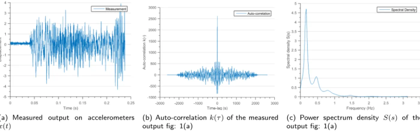
Sec-(a) Measured output on accelerometers x(t)
(b) Auto-correlation k(τ ) of the measured output fig: 1(a)
(c) Power spectrum density S(s) of the output fig: 1(a)
Figure 1: Different types of measurements for estimation of Modal parameters in OMA
tion 3 details the changes made to current algorithms and in-troduces the BIC. Section 4 demonstrates the capabilities of the algorithm on a simulated dataset and finally section 5 con-cludes the paper with future outlook.
2 OPERATIONAL MODAL ANALYSIS
As stated earlier the operational modal analysis is an output dependent modal identification technique. The only thing re-quired is the measurement from the accelerometers placed on the structure. Figure 1(a) shows an example of ambient mea-surements x(t) on a structure. In almost all OMA algorithms the measurement x(t) is assumed to be generated from a ran-dom force excitation.
The following subsections describe the various time-domain subsection 2.1 and frequency-domain algorithms subsection 2.2 for performing OMA.
2.1 Time-domain OMA
In the time-domain a general auto-regression moving average (ARMA) model can be applied to the measurement x(t)[11]. Here, the modal parameters can be computed from the coef-ficients of polynomials in ARMA models[12].
If we assume that a second order differential (equation 1) com-pletely describes the system dynamics. Then Natural Excita-tion Technique [13] proves that the auto-correlation function
k(τ )in equation 2 can be written as sum of decaying sinu-soid’s as described by equation 3. The auto-correlation de-scribes the similarity between measurement as a function of time lag τ between them figure 1(b).
k(τ ) = Z
x(t)x(t − τ )dt (2)
Here, k(τ ) denotes the auto-correlation for random vector x(t) as a function of time lag τ .
k(τ ) =XAiexp(−λiτ )sin(Biτ ) (3)
Here, λi and Ai denotes the modal frequency and mode
shapes for the ithmode. The above coefficients are found by
minimizing the least square error between the measured k(τ ) from equation 2 and the predicted k(τ ) from equation 3. This process is very similar to the Least Square Complex Exponen-tial (LSCE)[14] [15] [1]algorithm developed for time-domain
EMA.
2.2 Frequency-domain OMA
If we assume the measurement x(t) to be a stationary ran-dom process, then according to bochner’s theorem [16] the
spectral density or power spectrum S(s) can be represented as equation 4.
S(s) = Z
k(τ )exp(−2πisTτ )dτ (4)
Here, S(s) is the power spectrum for the measurement x(t), where s lies in the frequency-damping plane. Figure 1(c) shows the power spectrum calculated for the measurement x(t)shown in figure 1(a).
Initially the Peak Picking technique (PP)[17]was used in the frequency-domain to identify modal frequencies and shapes. The PP technique is a very easy way to identify modes but
Measurement; eg. figure 1(a) Auto-correlation; eg. figure 1(b) Power Spectrum; eg. figure 1(c) x(t) k(τ ) =R x(t)x(t − τ )dt S(s) =R k(τ )exp(−2πisT
τ )dτ Assumption: Second Order Differential
k(τ ) =P Aiexp(−λiτ )sin(Biτ ) S(jω) = P ak(jω)
k
P bl(jω)l Assumption: Gaussian Mixture Model
x(t) = GP (0, covSM) k(τ ) =P wicos(2πµiτ )exp{−2π2σi2τ2} S(s) =P wi√1 2πσ2 i exp{ 1 2σ2 i (s − µi)2}
TABLE 1: Comparison of fitting functions
becomes inefficient for complex structures[18]. This gave rise to the Frequency Domain Decomposition (FDD) [19] where
modal frequency are denoted as the eigenvalues of spectral density matrix equation 5.
S(jω) = U ΣUH (5)
Here, modal frequencies and mode shapes can be derived from Σ and U respectively using FDD[19]or Enhanced-FDD [20]
.
Majority of frequency-domain algorithms in EMA fit a Rational Fractional Polynomial (RFP)[2] in the frequency domain for
modal identification[21] [22]. The Rational Fractional Polyno-mial equation 6 form can be derived if we assume the system to be second order differential equation 1.
S(jω) = P ak(jω)
k
P bl(jω)l
(6)
Here, the poles of the polynomial denote the modal frequen-cies, while other modal parameters can be derived from the coefficients akand bl. The coefficients of the polynomial can
be found by minimizing the least squared error. RFP based algorithms face problems since as the number of modes in-crease the matrix becomes ill-conditioned which gives rise to stability issues in prediction of modal parameters. In the next section we will drop the assumption of second order differ-ential system and treat the modal identification as a purely curve-fitting problem.
3 GAUSSIAN MIXTURE MODELS (GMM)
Two of the above mentioned OMA algorithms ”Natural Exci-tation Technique” in the time domain and ”Rational Fractional Polynomial” in the frequency domain, have a core assumption
of second order differential system. This assumption fails for non-linear systems and for cases where modal frequencies are very close. In the following section we propose to use Gaussian Mixture Models to fit the power spectrum curve. Scale location mixtures of Gaussian’s can approximate a curve to arbitrary precision with enough components[23]. Due
to the above property GMM’s are widely used in machine learning tasks such as speech recognition[24], financial
mod-elling[25], handwriting recognition[26]and many more.
Due to the formulation of GMM, the mean, standard deviation and weight information of the gaussian’s can be used to derive the modal frequency, damping and mode shape of the system respectively. For a positive half power spectrum the GMM will be equivalent to equation 7. S(s) = Q X i wi 1 p2πσ2 i exp{ 1 2σ2 i (s − µi)2} (7)
Here, µi, σi and wi are the mean, standard deviation and
weight respectively of the ith gaussian. While, Q denotes the number of gaussians used in the GMM. The mean, stan-dard deviation and weight can be found by minimizing the least square error between measured power spectrum and predicted power spectrum S(s). The method to estimate Q will be explained in more detail in subsection 3.1.
The GMM model in the frequency-domain can be transformed to perform covariance-driven modal identification using the equation 4. If we assume x(t) to be a stationary random process then using to equation 7 and equation 4 we can get equation 8 in the time domain[27].
k(τ ) = Q X i wicos(2πµiτ )exp{−2π2σ2iτ 2} (8)
weight respectively of the ithgaussian. While, Q denotes the
number of gaussians used in the GMM, τ is the time lag be-tween two measurement instances. The parameters can be found by minimizing the least squared error.
Moreover, if we assume that x(t) is a zero-mean gaussian process, then we can transform GMM in frequency-domain to time-domain. The equation 7 and equation 8 are equivalent to fitting a zero-mean gaussian process with a spectral mixture covariance function[28].
x(t) = GP (0, covSM(t, t0)) (9)
Here, GP denotes a gaussian process[29], while cov SM
rep-resents a spectral mixture covariance function which resem-bles equation 8[28].
We would like to emphasize that keeping the computational complexities aside, fitting a spectral mixture gaussian process in time-domain equation 7, fitting equation 8 for covariance-driven modal identification and fitting a GMM equation 7 in the frequency-domain are equivalent. In fact the initial idea of this paper was to fit a Gaussian Process (GP) in the data domain, but GP’s are computationally heavy and we achieved a good accuracy by fitting the GMM in frequency domain. Refer to table 1 for a more comprehensive view at various fitting func-tions.
3.1 Bayesian Information Criteria (BIC)
While the modal parameters can be chosen by minimizing the least square error, how to choose the number of modes is a recurring question in several OMA algorithms. This problem is partially resolved by using stabilization diagrams or mode identification functions[21] [30] [31]. But in practical
situa-tions engineering judgement is required to estimate the opti-mal modal order.
Here, we use the Bayesian Information Criteria (BIC) [32]
which penalises more complex models to estimate the param-eter Q in equation 7. It has been shown earlier that the BIC when applied to GMM’s does not underestimate the true num-ber of components[33].
BIC(Q) = n ln(M LE) + k ln(n) (10)
Here, n denotes the number of data-points to fit, M LE notes the maximum likelihood estimation of the fit and k de-note the number of free parameters to fit. The BIC per-forms a trade-off between the data-fit term n ln(M LE) and the complexity penalty term k ln(n), basically penalizing for over-fitting. Lowest value of BIC is preferred.
4 RESULTS
In this section we conduct experiments, applying our approach on a simple 3 degree of freedom system with close by modes. As stated earlier in section 3 we fit a Gaussian Mixture Model (GMM) on the spectral density. Later we will compare the Bayesian Information Criteria to find the optimal value of num-ber of gaussians for the measurement.
The toolbox used for this paper is Matlab’s Curve Fitting Tool-box[34]. All experiments were performed on an Intel quad-core processor with 4Gb RAM. Using the curve fitting toolbox the fitting can be performed by a few lines of code. When com-pared to other frequency-domain techniques like RFP which suffer from ill-conditioned matrices, the GMM technique is highly stable and finds the coefficient’s in seconds.
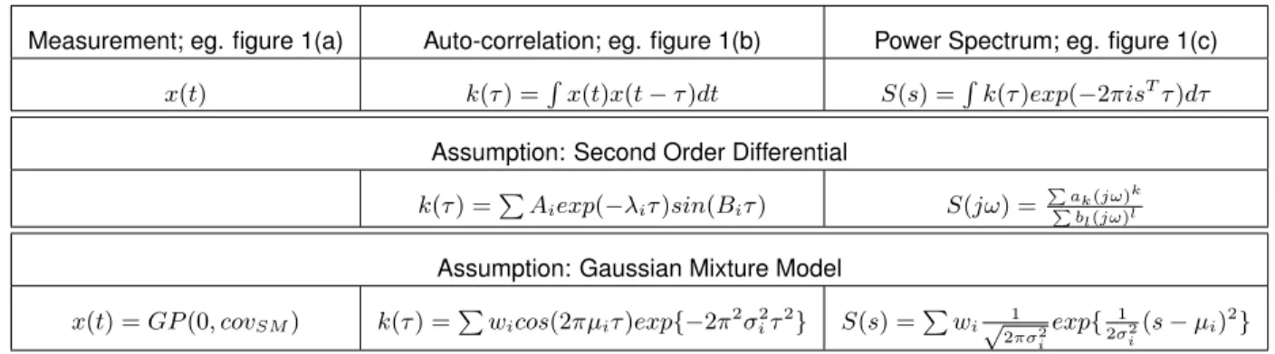
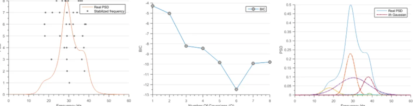
Figure 2(a) shows the stabilization diagram with increasing number of gaussians Q. We can observe that as the num-ber of Q increases the algorithm starts finding better and bet-ter modes. We can also observe that there are three modes which start stabilizing from Q = 5. The, figure 2(b) shows the BIC criterion with increasing number of gaussian’s Q. We can see that that the BIC is minimum for Q = 6 and hence if we add anymore gaussian’s for our dataset we will be performing over-fitting.
Figure 2(c) shows the 6 constituent gaussians which repre-sent the Q = 6 case. The three principal peaks reprerepre-sent the modal frequencies of the system, these correspond to the stabilized frequencies from figure 2(a). The remaining three peaks are there to compensate for the spectral density not explained by the three principal peaks.
In the current setting of the GMM model we only propose a quick and easy way to identify the most important frequen-cies of a structural system. Neither the mode shapes nor the damping ratios are estimated in the current format. As can be observed from figure 2(c) the mode shapes are not only dependent on the principal gaussian’s but also on the neigh-bouring gaussian’s. Since some part of the spectral density is defined by non-stabilized gaussian’s, in future we would like to derive a method to estimate mode-shape and damping ra-tio such that the contribura-tions of neighbouring gaussian’s are also taken into account.
5 CONCLUSION
In this paper we have proposed to identify model frequen-cies of a system by curve-fitting a mixture of gaussians in the frequency domain. While the common assumption that the structure can be modelled as a MDOF second order differen-tial system causes stability issues in presence of non-linear systems. The GMM model is mathematically stable, gives re-sults in seconds and can fit a function upto arbitrary accuracy. Moreover we introduce the BIC to identify the optimum
num-(a) Stabilization diagram with increasing number of gaussians Q, the dots denote the stabilized frequencies. We can observe that as the number of Q increases the algorithm starts finding better and better modes.
(b) The BIC criterion with increasing num-ber of gaussian’s Q. We can see that that the BIC is minimum for Q = 6 and hence if we add anymore gaussian’s for our dataset we will be performing over-fitting
(c) Distribution of gaussians for Q = 6. We can see that the three modal frequen-cies have majority of the participation in representing the spectral density.
Figure 2: Results of applying GMM on a Spectral density
ber of gaussians and perform a trade-off between accuracy of fit and over-fitting.
Without doubt this is very nascent stage of application of GMM for system identification and there remains problems such as identification of mode-shape and damping ratio in this algo-rithm. We wish to tackle these problems in the future. We also wish to apply the algorithm on a real world dataset and compare with respect to other time domain and frequency do-main techniques.
ACKNOWLEDGMENTS
The author’s are really indebted to the encouragement and support provided by, Jonatan Santiago Tonato, Emmanuel Rachelson, Michele Colombo and Sebastien Blanc.
REFERENCES
[1] Guillaume, P., Verboven, P., Vanlanduit, S., Van Der Auweraer, H. and Peeters, B., A poly-reference
implementation of the least-squares complex frequency-domain estimator, Proceedings of IMAC, Vol. 21, pp. 183–192, 2003.
[2] Richardson, M. H. and Formenti, D. L., Parameter
es-timation from frequency response measurements using rational fraction polynomials, Proceedings of the 1st in-ternational modal analysis conference, Vol. 1, pp. 167– 186, Union College Schenectady, NY, 1982.
[3] Peeters, B., Van der Auweraer, H., Pauwels, S. and Debille, J., Industrial relevance of Operational Modal
Analysis–civil, aerospace and automotive case histories,
Proceedings of IOMAC, the 1st International Operational Modal Analysis Conference, 2005.
[4] Shahdin, A., Morlier, J., Niemann, H. and Gourinat, Y., Correlating low energy impact damage with changes
in modal parameters: diagnosis tools and FE validation, Structural Health Monitoring, 2010.
[5] Rainieri, C., Fabbrocino, G. and Cosenza, E.,
Auto-mated Operational Modal Analysis as structural health monitoring tool: theoretical and applicative aspects, Key Engineering Materials, Vol. 347, pp. 479–484, Trans Tech Publ, 2007.
[6] Lindsay, B. G. et al., The geometry of mixture
likeli-hoods: a general theory, The annals of statistics, Vol. 11, No. 1, pp. 86–94, 1983.
[7] McLachlan, G. and Peel, D., Finite mixture models, John
Wiley & Sons, 2004.
[8] Blumer, A., Ehrenfeucht, A., Haussler, D. and War-muth, M. K., Occams razor, Readings in machine
learn-ing, pp. 201–204, 1990.
[9] Schwarz, G. et al., Estimating the dimension of a model,
The annals of statistics, Vol. 6, No. 2, pp. 461–464, 1978. [10] Roeder, K. and Wasserman, L., Practical Bayesian
den-sity estimation using mixtures of normals, Journal of the American Statistical Association, Vol. 92, No. 439, pp. 894–902, 1997.
[11] Ljung, L., System identification, Signal Analysis and
Prediction, pp. 163–173, Springer, 1998.
[12] Andersen, P., Identification of civil engineering
struc-tures using vector ARMA models, Ph.D. thesis, unknown, 1997.
[13] James III, O. and Came, T., THE NATURAL
EXCI-TATION TECHNIQUE (NEXT) FOR MODAL PARANI-ETER EXTRACTION FROM OPERATING STRUC-TURES, 1995.
[14] Spitznogle, F. R. and Quazi, A. H., Representation and
Analysis of Time-Limited Signals Using a Complex Expo-nential Algorithm, The Journal of the Acoustical Society of America, Vol. 47, No. 5A, pp. 1150–1155, 1970. [15] Ibrahim, S. and Mikulcik, E., A method for the direct
identification of vibration parameters from the free re-sponse, 1977.
[16] Bochner, S., Lectures on Fourier Integrals.(AM-42),
Vol. 42, Princeton University Press, 2016.
[17] Gade, S., Møller, N., Herlufsen, H. and Konstantin-Hansen, H., Frequency domain techniques for
opera-tional modal analysis, 1st IOMAC Conference, 2005. [18] Zhang, L., An overview of major developments and
is-sues in modal identification, Proc. IMAC XXII, Detroit (USA), pp. 1–8, 2004.
[19] Brincker, R., Zhang, L. and Andersen, P., Modal
identi-fication from ambient responses using frequency domain decomposition, Proc. of the 18*International Modal Anal-ysis Conference (IMAC), San Antonio, Texas, 2000. [20] Brincker, R., Ventura, C. and Andersen, P.,
Damp-ing estimation by frequency domain decomposition, 19th International Modal Analysis Conference, pp. 698–703, 2001.
[21] Allemang, R. J. and Brown, D., A unified matrix
polyno-mial approach to modal identification, Journal of Sound and Vibration, Vol. 211, No. 3, pp. 301–322, 1998. [22] Chauhan, S., Martell, R., Allemang, R. and Brown, D.,
Unified matrix polynomial approach for operational modal analysis, Proceedings of the 25th IMAC, Orlando (FL), USA, 2007.
[23] Plataniotis, K. N. and Hatzinakos, D., Advanced
Sig-nal Processing Handbook Theory and Implementation for Radar, Sonar, and Medical Imaging Real Time Sys-tems.
[24] Stuttle, M. N., A Gaussian mixture model spectral
repre-sentation for speech recognition, Ph.D. thesis, University of Cambridge, 2003.
[25] Xu, L. and Jordan, M. I., On convergence properties of
the EM algorithm for Gaussian mixtures, Neural compu-tation, Vol. 8, No. 1, pp. 129–151, 1996.
[26] Bishop, C. M., Pattern recognition, Machine Learning,
Vol. 128, 2006.
[27] Wilson, A. G. and Adams, R. P., Gaussian Process
Ker-nels for Pattern Discovery and Extrapolation Supplemen-tary Material.
[28] Wilson, A. G. and Adams, R. P., Gaussian Process
Ker-nels for Pattern Discovery and Extrapolation., ICML (3), pp. 1067–1075, 2013.
[29] Rasmussen, C. E., Gaussian processes in machine
learning, Advanced lectures on machine learning, pp. 63–71, Springer, 2004.
[30] Williams, R., Crowley, J. and Vold, H., The multivariate
mode indicator function in modal analysis, International Modal Analysis Conference, pp. 66–70, 1985.
[31] Shih, C., Tsuei, Y., Allemang, R. and Brown, D.,
Com-plex mode indication function and its applications to spa-tial domain parameter estimation, Mechanical systems and signal processing, Vol. 2, No. 4, pp. 367–377, 1988. [32] Findley, D. F., Counterexamples to parsimony and BIC,
Annals of the Institute of Statistical Mathematics, Vol. 43, No. 3, pp. 505–514, 1991.
[33] Leroux, B. G. et al., Consistent estimation of a
mix-ing distribution, The Annals of Statistics, Vol. 20, No. 3, pp. 1350–1360, 1992.
[34] MathWorks, I., Curve fitting toolbox 1: user’s guide,