HAL Id: hal-02538041
https://hal.archives-ouvertes.fr/hal-02538041
Submitted on 9 Apr 2020
HAL is a multi-disciplinary open access
archive for the deposit and dissemination of
sci-entific research documents, whether they are
pub-lished or not. The documents may come from
teaching and research institutions in France or
abroad, or from public or private research centers.
L’archive ouverte pluridisciplinaire HAL, est
destinée au dépôt et à la diffusion de documents
scientifiques de niveau recherche, publiés ou non,
émanant des établissements d’enseignement et de
recherche français ou étrangers, des laboratoires
publics ou privés.
Applying Parametric Model-Checking Techniques for
Reusing Real-time Critical Systems
Baptiste Parquier, Laurent Rioux, Rafik Henia, Romain Soulat, Olivier Henri
Roux, Didier Lime, Étienne André
To cite this version:
Baptiste Parquier, Laurent Rioux, Rafik Henia, Romain Soulat, Olivier Henri Roux, et al.. Applying
Parametric Model-Checking Techniques for Reusing Real-time Critical Systems. 5th International
Workshop on Formal Techniques for Safety-Critical Systems (FTSCS 2016), Nov 2016, Tokyo, Japan.
�10.1007/978-3-319-53946-1_8�. �hal-02538041�
Techniques for Reusing Real-time Critical
Systems
?Baptiste Parquier1,2, Laurent Rioux1, Rafik Henia1, Romain Soulat1, Olivier
H. Roux2, Didier Lime2, and ´Etienne Andr´e2,3
1 THALES Research & Technology, 1 avenue Augustin Fresnel, 91120 Palaiseau,
France
2 IRCCyN, 1 rue de la No¨e, 44300 Nantes, France 3
Universit´e Paris 13, Sorbonne Paris Cit´e, LIPN, CNRS, UMR 7030, F-93430, Villetaneuse, France
Abstract. Due to the increase of complexity in real-time safety-critical systems, verification and validation costs have significantly increased. A straightforward way to reduce costs is to reuse existing systems, adapting them to new requirements, so as to avoid new costly developments. Our aim is to verify during the development strategy definition phase whether the existing products can be reused and adapted for a new customer, by identifying key parameters to be tuned in order to reuse existing products. Performing efficient verification is therefore crucial.
In this paper, we focus on the performance requirement aspects. Nowa-days, model-checking techniques have improved significantly to verify the performances of real-time systems. However, model-checking cannot address real-time systems where some timing constants are unknown or uncertain. Parametric model-checking leverage this shortcoming by iden-tifying parameter ranges for which the system is correct. We report here on an experiment of the evaluation of the use of these formal techniques applied to automatize the synthesis of good parameter ranges for system reuse in the setting of the environment requirements for an aerial video tracking system.
Keywords: Real-time Systems · Safety-Critical Systems · Formal Meth-ods · Parametric Verification · Performance Verification · Case Study · Avionics
1
Introduction
Performance verification is a common discipline in system and software engi-neering. In practice, it is very common to spend a lot of effort in performance
?This paper is the author version of the paper of the same name published in the
proceedings of the 5th International Workshop on Formal Techniques for Safety-Critical Systems (FTSCS 2016), Tokyo, Japan, November 2016. This work is par-tially supported by the ANR national research program ANR-14-CE28-0002 PACS (“Parametric Analyses of Concurrent Systems”).
engineering especially for certified products. Standards specify a complete and precise safety process to follow in order to be certified (e. g., DO-178C in the avionics domain). There is a need to reduce the time and efforts related to de-sign such real-time systems considering performance requirements. We would like to experiment and verify if the current state of the art on performance ver-ification tools are able to cope with industrial needs. We will not address the whole performance engineering process. We will focus on the performance verifi-cation in a particular context: an industrial company plans to reuse an existing real-time safety-critical system for the needs of a new client to cut costs and delays. However, this client is coming with its own performance requirements that differs from what the system was originally designed for. Our use case is an aerial video tracking device. Its mission is safety-critical for the whole system and, therefore, has to be certified according to the DO-178C standard.
To this end, we have to demonstrate the software architecture meets the performance requirements, which implies that the system has to satisfy all the deadline requirements in all (and in particular the worst) situations.
A conventional way at THALES—but also in other industrial companies— to tackle this problem is to evaluate the performance of the current system. The system is taken as is and if it satisfies the client performance requirements, the system can be reused as it stands. If not, experts check how to modify environment parameters—typically sources of activation of the system—and try to identify a new configuration where the system can meet its new requirements. This is time consuming and costly. Therefore, generally only few configurations are tested and evaluated, and quite often, none of them meets the requirements. As a consequence when the activity is seen as too costly, the “reuse” strategy is dropped.
We report here on an experimentation to apply formal techniques on an aerial video tracking system by THALES, in a way to tool-up the identification of the good environment parameters to reuse the system. Our methodology is as follows:
1. We first identified the most appropriate formalisms and formal techniques to validate the performance and identify the good environment parameters: we chose to use parametric stopwatch automata (PSwAs) and parametric stopwatch Petri nets (PSwPNs), two formalisms for modeling and verifying preemptive real-time systems with parameters. These two formalisms benefit from state-of-the-art model-checkers (IMITATORfor PSwAs and Rom´eo for PSwPNs).
2. We then devised a way to model the system needed for performance valida-tion, using the identified formalisms.
3. We then studied how to measure the trust in the results produced by IMI-TATORand Rom´eo: In this regard, we exploit diversity: the use of several
techniques giving the very same results is a great source of confidence. Nev-ertheless, diversity can only be reached if the alternatives used are truly different and cannot both fail due to some common weaknesses.
Organization of the Paper. Section 2 presents the aerial video tracking system developed by THALES, and its new requirements.Section 3 presents the state of the art of available verification techniques, in particular formal methods using parameterization.Section 4introduces the tools Rom´eo andIMITATOR respec-tively for parametric stopwatch Petri nets and parametric stopwatch automata. Section 5provides the modeling of the case-study into both formalisms. Finally we present experimental results inSection 6and we conclude withSection 7.
2
Industrial Case-Study
2.1 SpecificationsThis case-study is an aerial video tracking system designed by THALES, used in intelligence, surveillance, reconnaissance, tactical and security applications. Fig. 1presents the two major functions of this system:
1. The video frame processing function, which receives frames from the camera and sends them to the cockpit to be displayed for the pilot.
2. The tracking and camera control function, which gives the control commands to the camera from the aircraft sensor data. The study focuses on this part of the system.
The objective of the tracking and camera control function is to control the camera position according to the plane trajectory. The camera has to always focus on the same target, whatever the plane trajectory is.
The system is characterized by strict constraints on timing. One major tim-ing problem consists in calculattim-ing the timtim-ing latencies for the functions in the “Tracking and Camera control” part.
Fig. 1. Organization of the aerial video tracking system
“Tracking and Camera control” is decomposed in 4 subfunctions: Processing (T2), Target position prediction (T5), Tracking control (T6) and Camera control (T7). All sub-functions share the same computing resource, i. e., work on the same CPU.Fig. 2illustrates how all those sub-functions communicate with each other and how much time they require on the computing resource. (The red arrow in Fig. 2is not considered for now, and will be used later on.)
Fig. 2. Tracking and camera control: time description
The system has the following characteristics:
– All tasks are triggered by the arrival of data at their inputs; – There is a preemptive scheduling for the computing resource; – Tasks are prioritized in this order: T2 > T6 > T5 > T7.
Let us now introduce various definitions.
Definition 1. A period τ is the duration after which a periodic phenomenon repeats itself.
Definition 2. A jitter is the maximal delay of activation compared to the peri-odic arrival of the event causing this activation.
Definition 3. A time offset ω is the time lag between an event and a time reference—taken arbitrarily.
Definition 4. In a system, a stimulus is an external activation that periodically sends a signal to one or multiple tasks. It is fully characterized by: 1. A period, 2. A jitter, 3. A time offset.
Example 1. In our case-study, there are two stimuli as shown inFig. 2:
– The first one activating T6—tracking control: period 100 ms, jitter j, no offset—this stimulus is chosen as reference,
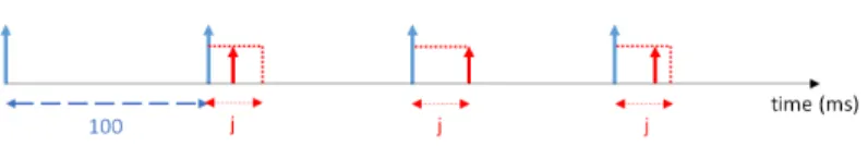
Fig. 3. A 30 ms jitter on a 100 ms period stimulus
Example 2. Fig. 3 illustrates a periodic stimulus with a period of 100 ms and a jitter j, that activates a task. The periodic stimulus sends data to the task in order to activate it (blue arrows inFig. 3). Because of the jitter, the activation of the task happens between 0 and j time units after the stimulus (red arrows). The jitter j represents a potential delay due to the communication network in the aircraft. It is not something that can be determined at design time: the best a designer can do is to take into account that there will be a possible delay in the final system and ensure the system will behave according to the requirements whatever the jitter is. Until now, system environment ensured that:
j = 30 ms
The offset ω might be used to change the reference between T6’s and T2’s activations. An offset is something the designer can tune to ensure the system good behavior.
2.2 Main Objective
Our main objective is to reuse an existing system for new customers, which means the system has to meet all new performance requirements. More precisely, in this experiment, we consider the situation where a new customer wants to modify the following requirement to the aerial video tracking system: “The end-to-end latency between the activation of task T6 and the termination of task T7 shall be lower than 80 ms.” The new end-to-end latency requirement is depicted in red inFig. 2.
Our aim is to compute new timing specifications of the system so that this additional requirement can be met. However, the heart of the system must not change. As the system is expected to be reused as is, we can only modify the timing specifications of external activations: tune the offset between stimuli, or change the jitter requirements.
2.3 Our Constraints: a Parametric Approach
In our case study, jitter and offset can be seen as parameters. Moreover, even timing properties can be expressed parametrically, as timing constraints make sense only in the context of a given concrete environment. For example, a maxi-mal delay of the system response has to be at most two times the minimaxi-mal delay, or the transmission time in the communication protocol could be left as a pa-rameter. Performing non-parametric model-checking of the systems for different
concrete values is difficult and leads to state-space explosion. The possibility to specify parametric timing constraints is then a great opportunity that allows to evaluate timing performances of real-time systems independently of their par-ticular implementation.
We summarize the main needs for a parametric approach:
– Parameters allow to cope with the early uncertainties in developing an in-dustrial system;
– Parameters allow to investigate robustness of some of the design choices; – If the system is proven wrong, the whole verification process has to be carried
out again;
– Considering a wide range of values for constants allows for a more flexible and robust design.
3
Related Works
3.1 Response Time and Latency Analysis
As mentioned in [SSL+13], many research papers have already addressed the problem of parametric schedulability analysis, especially on single processor sys-tems. Bini and Buttazzo [Bin04] proposed an analysis of fixed priority single processor systems, which is used as a basis for this paper.
Parameter sensitivity can be also be carried out by repeatedly applying clas-sical schedulability tests, like the holistic analysis [PGGH98]. One example of this approach is used in the Mast tool [GHGGPGDM01], in which it is possi-ble to compute the slack (i. e., the percentage of variation) with respect to one parameter for single processor and for distributed systems by applying binary search in that parameter space [PGGH98].
A similar approach is followed by the SymTA/S tool [HHJ+05], which is based on the event-stream model [RE02]. Another interesting approach is the Modular Performance Analysis (MPA) [WTVL06], which is based on Real-Time Calculus. In both cases, the analysis is compositional, therefore less complex than the holistic analysis. In [LPPR13], a real time system is modeled using a high level variant of timed automata including design timed parameters and is analyzed using the UPPAAL tool. Nevertheless, these approaches are not fully parametric, in the sense that it is necessary to repeat the analysis for every combination of parameter values in order to obtain the schedulability region.
3.2 Parametric Formalisms for Real-time Systems
The literature proposes mainly two formalisms to model and verify systems with timing parameters: parametric timed automata [AHV93] and parametric time Petri nets [TLR09]. Both formalisms are subject to strong undecidability results, even with low numbers of parameters [Mil00], syntactic restrictions such as strict constraints [Doy07], or with restricted parameter domains, such as bounded rationals [Mil00], or (unbounded) integers [AHV93] (see [And16] for a survey).
Undecidability is not necessarily a problem: semi-algorithms were defined (e. g., [AHV93], [ACEF09], [JLR15]) and safe under-approximations were also proposed (e. g., [ALR15], [JLR15]).
For many real-time systems, in particular when subject to preemptive schedul-ing, these formalisms are not expressive enough. As a consequence, we therefore use extensions of parametric timed automata and parametric time Petri nets augmented with stopwatches, yielding parametric stopwatch automata [SSL+13], and parametric stopwatch Petri nets [TLR09].
To the best of our knowledge, the only tools using as basis formalism these two formalisms are IMITATOR [AFKS12] for parametric stopwatch automata, and Rom´eo [LRST09] for parametric stopwatch Petri nets. In this work, we evaluate the capabilities of both tools using the industrial case study.
4
Tools
We briefly present both tools in the following. Using tools is an opportunity to increase the confidence in our results. We believe this offers us the diversity we seek for in our approach, because the tools are developed by different teams, and based on different theories: parametric stopwatch Petri nets vs. parametric stopwatch automata, that implies different models.
By doing that, the confidence one can have in both tools increases consider-ably: if both tools give the same results, the odds that they are both wrong is clearly very low, and therefore the confidence is high.
4.1 Rom´eo
Rom´eo4 [LRST09] is a software studio for parametric analysis of time Petri nets and some of their hybrid extensions (such as parametric stopwatch Petri nets). It is available for Linux, MacOSX and Windows platforms and consists of a graphical user interface (GUI) to edit and design PSwPNs, and a computation engine.
Rom´eo supports the use of parametric linear expressions in the time intervals of the transitions, and allows to add linear constraints on the parameters to restrict their domain. Finally, Rom´eo provides a simulator and an integrated TCTL model-checker [BGR09].
4.2 IMITATOR
IMITATOR5 [AFKS12] is a software for parametric verification and robustness analysis of real-time systems. It relies on the formalism of networks of parametric timed automata, augmented with integer variables and stopwatches. Parameters can be used both in the model and in the properties.
IMITATORis fully written in OCaml, and makes use of the Parma Polyhedra Library [BHZ08]. It is available under the GNU General Public License.
4
http://romeo.rts-software.org
5
5
Modeling the Case-Study
Modeling the system in both tools was one of the challenges of this work. Each theory has its particularities, and translating the case-study specifications ac-cording to the associated theory was sometimes problematic. This part presents the modeling choice we made to obtain an equivalent model of the aerial video tracking system, both with Rom´eo andIMITATOR.
Modeling reentrancy In our models, we decompose the task T6—tracking control— in three different tasks:
– T6 1, duration [4, 4] ms – T6 2, duration [9, 10] ms – T6 3, duration [4, 5] ms
This decomposition simplifies the analysis of the transmission of data between T6, T5 and T7—shown Fig. 2. Indeed, with this modification there is no more transmission inside a task. However, the system’s behavior needs to stay unmod-ified: there can not be two cycles T6 1 to T6 3 overlapping. After an activation of T6—i. e., T6 1—it is impossible to have a new one before its termination—i. e., T6 3 termination.
Definition 5. We define a cycle between two tasks T and T0—T causing the activation of T0—as the the time elapsed between the activation of task T and
the termination of T0 caused by this activation.
The phenomenon of overlapped cycles is called reentrancy, e. g., when there are at least two T6’s activation before any T7’s termination.
5.1 Rom´eo
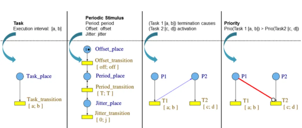
We give in Fig. 4 the rules that we use to translate the aerial video track-ing system into PSwPNs. Each element needed in the system—task, stimulus, synchronization (blue arc) and priority (red arc)6—is translated (in that or-der). The whole formal model is constructed by linking by an arc the elements (pattern) constituting the system. As an example, for the periodic task T 2, the Periodic Stimulus pattern is linked to the Task pattern by an arc between J itter transition to Task place. According to these few rules, we obtained a PSwPN net modelling the case-study.
Remark 1. In Rom´eo, there is no explicit time unit: it is inherent to the model. Every duration in the case-study is in ms, so the time value given by Rom´eo will be in ms.
6
The use of timed (resp. discrete) inhibitor arc (red arc) leads to the modeling of preemptive (resp. non-preemptive) scheduling.
Fig. 4. Translating the system (top) into Rom´eo (bottom)
In this model, there are two parameters: jitter —corresponding to the maxi-mal delay j of the first stimulus defined inSection 2.1—and offset —corresponding to the offset ω of the second stimulus.
To be consistent with the case-study, the following constraints are defined: jitter ≤ 30 & offset ∈ [0, 40) (1) Remark 2. There is no need for a larger range for the offset: T2 is activated every 40 ms (periodic stimulus), so we review all possible cases with these bounds.
To be able to compute a latency, an observer is needed.7 An observer is another time Petri net linked to the initial net that needs to be observed. It does not change the behavior of the observed part, and—by asking the right property to the model-checker and thanks to a parameter—it allows to compute the worst latency between two tasks.
5.2 IMITATOR
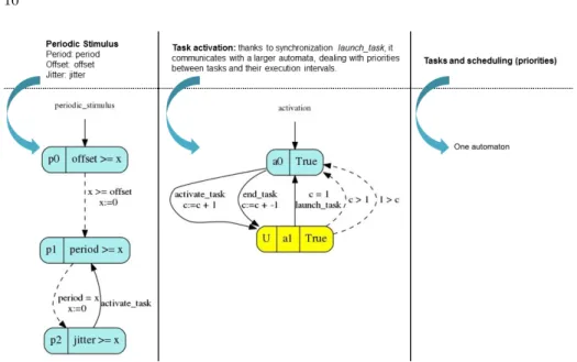
We give inFig. 5the translation rules to build theIMITATORmodel. Constraints on the model are defined in the same way as with Rom´eo inEq. (1). The whole formal model is constructed by synchronizing the elements (pattern) constitut-ing the system. The IMITATOR synchronization model is such that all PSwAs declaring an action must synchronize together on this action. As an example, for the periodic task T 2, the Periodic Stimulus pattern is synchronized with the Task pattern by the activate task action.
Remark 3. As in Rom´eo, there is no explicit time unit inIMITATOR.
7
Observers (also called testing automata) were studied in [ABBL98,ABL98], and a library of common observers was proposed in [And13].
Fig. 5. Translating the system (top) into IMITATOR (bottom)
6
Experiment Results
6.1 HardwareThe computation was conducted on a regular personal computer running Linux 64 bits 3.10 GHz and 4 GiB memory. Models and experiment results are available atwww.imitator.fr/FTSCS16.
For our analysis, as explained in Section 2.2, we are interested in checking that the worst-case end-to-end latency—from activation of the Tracking control task to termination of the Camera control task as defined inSection 2.1—does not exceed 80 ms.
6.2 Worst-case Scenario
We have computed the worst latency for the basic configuration: i. e., with a 30 ms jitter – the activation of T6 in Fig. 2 may happen between 0 and 30 ms after the arrival of the stimulus. If this worst latency between the T6’s activation and T7’s termination is less than 80 ms, this configuration of the system meets the requirements.
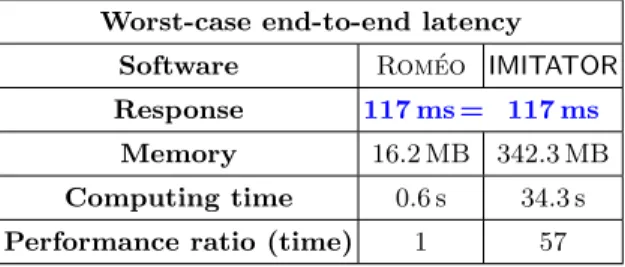
Table 1 presents the results obtained with both Rom´eo andIMITATOR. In this table and the following, the Performance ratio denotes a comparison be-tween the computing times of the two tools. The fastest is taken as reference.
Both tools give the same result: the worst time is 117 ms. It is really re-assuring. As explained in Section 4, this allows the designer to have a strong confidence in this result.
Table 1. Case-study: 30 ms jitter, no offset Worst-case end-to-end latency
Software Rom´eo IMITATOR Response 117 ms = 117 ms
Memory 16.2 MB 342.3 MB Computing time 0.6 s 34.3 s Performance ratio (time) 1 57
The used tools are able to produce traces for the worst cases. This is of prime interest for someone designing a system as it allows him to understand the existing bottlenecks and to be able to easily address them.
Fig. 6shows this worst-case scenario. The worst time is reached because of reentrancy when all tasks have their longest duration. Indeed, the task T7—the one with the lowest priority—does not have the time to end before the launching of a new cycle. It is then preempted by all the other tasks. The reentrancy is possible because of the jitter. There are only 70 ms between both activations of task T6 (tracking control).
Fig. 6. Gantt chart of the worst-case scenario
Moreover, the end-to-end delay requirement given by the client is not met.
117 ms > 80 ms
In the next part, we investigate if the modification of environment parameters could fix it.
6.3 Exploitation of Parameters
In this part, we are interested in addressing the capabilities of the tools to explore different parameter valuations in order to meet requirements. As presented in Section 2, to modify the external sources of activations—i. e., stimuli—we have two parameters we can operate on: the offset ω between the stimuli, and the jitter j before the activation of T6—tracking control. As a consequence, the designer is allowed to change the value of the offset in order to meet the end-to-end requirements. Otherwise, (s)he has to fix the maximal jitter the system can tolerate according to the same requirements.
The results (condition on both parameters ω and j) of Table 4 are more general and covers the results of the previous two. However,Table 2andTable 3 allow to compare the tools and to understand the compromise between the rele-vance of the result and the memory and the computing time required to obtain this result.
Offset Only. We are now interested in finding a constraint on the offset such that the 80 ms requirement is met. The observer is set to check that the end-to-end delay is below 80 ms. The offset between the two tasks is set as a parameter. The model checkers will produce a constraint on the offset such that the require-ment is always met.
Both model-checkers output ⊥, which denotes that no parameter valuations are such that the system meets the performance requirement. This means that no offset valuation can satisfy this requirement.
Table 2. Case-study: 30 ms jitter, parametric offset Worst-case end-to-end latency
Software Rom´eo IMITATOR wt ≤ 80 ms ⊥ = ⊥
Memory 64.0 MB 1,816 MB Computing time 3.3 s 3 min 35 s Performance ratio (time) 1 65
Remark 4. We have run a full analysis, performed by parameterizing both the offset and the end-to-end delay in the observer: this analysis, in fact, showed that no matter the offset, the worst case will always be 117 ms.
This ability to produce a negative result is also of prime interest for a sys-tem architect. It allows to reduce the design exploration time. In this case, the architect knows that tweaking the offset will never be successful.
Since acting on the offset was not enough, reducing the jitter’s specification becomes essential.
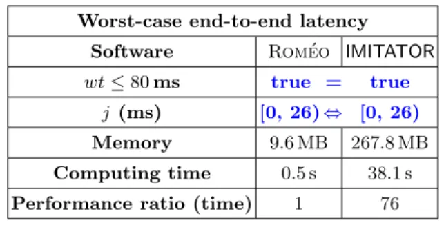
Reducing the Jitter. In this part, we explore another part of the design space: reducing the jitter. We are interested in finding jitter valuations that allows the system to meet its end-to-end maximal delay requirement. If we find a working configuration, we will take the highest authorised jitter’s value to put in the new requirements: it gives more flexibility to the system, allowing more flexibility for the external sources of events.
Jitter Only. In this part, we only use one parameter for the jitter’s value: j ∈ [0, 30] ms, the offset is set at ω = 0
Table 3. Case-study: parametric jitter j, no offset, wt ≤ 80 ms Worst-case end-to-end latency
Software Rom´eo IMITATOR wt ≤ 80 ms true = true
j (ms) [0, 26) ⇔ [0, 26)
Memory 9.6 MB 267.8 MB Computing time 0.5 s 38.1 s Performance ratio (time) 1 76
Once again, the results are still the same for both tools. According toTable 3: to meet its requirement, the system shall have a jitter j ∈ [0, 26) ms if the offset is left at ω = 0.
However, reducing the jitter can be expensive. We will investigate the possi-bility to have a higher jitter value by allowing a different offset ω.
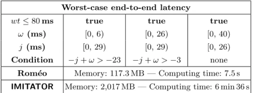
Offset and Jitter. In this part, we parametrize both the offset ω, and the jitter j—there are now two parameters in our models. To reduce the state-space, we add the following constraints:
ω ∈ [0, 40) ms & j ∈ [0, 30] ms (2) InTable 4are the results we obtained using this configuration: once again, both tools agreed.
For a system architect point of view, having the full constraints allows to make smart industrial choices. With these results, one of the smartest thing to do in order to have worst time ≤ 80 ms is, for example, to use 6 ms offset with 28 ms jitter. These two values are allowed by the results model-checkers gave us, and it is one of the highest jitter we can have.
Table 4. Case-study: 2 parameters (jitter j & offset ω), wt ≤ 80 ms Worst-case end-to-end latency
wt ≤ 80 ms true true true ω (ms) [0, 6) [0, 26) [0, 40)
j (ms) [0, 29) [0, 29) [0, 26) Condition −j + ω > −23 −j + ω > −3 none
Rom´eo Memory: 117.3 MB — Computing time: 7.5 s IMITATOR Memory: 2,017 MB — Computing time: 6 min 36 s
6.4 Tool Comparison
In our experimentations, Rom´eo has always performed better than IMITATOR
in terms of time and memory consumption. Therefore, Rom´eo seems to be a promising tool for future industrial use. It would be interesting to know why there is such a gap between these model-checkers, although they use a very similar notion of symbolic state, and a common internal representation using the Parma Polyhedra Library [BHZ08]. Here are some hypotheses:
– Both PSwAs and PSwPNs use clocks, i. e., real-valued variables. The number of clocks significantly impacts the model checking performance. A main dif-ference is that clocks are created statically in PSwAs (hence inIMITATOR), whereas they are dynamic in PSwPNs (hence in Rom´eo) and are therefore fewer in this latter case.
– The reentrancy phenomenon is well managed in Rom´eo, thanks to the Petri net theory—it is just multiple tokens in one place—whereas in IMITATOR, the reentrancy is made possible by adding variables and automata, which necessarily impacts the efficiency.
In addition, note that the distributed capabilities ofIMITATORwere not used in our comparison.
Nevertheless,IMITATORand Rom´eo gave us the same results: this is crucial for confidence in our results. Tool redundancy is used in some certification pro-cesses to lower the certification level needed for each tool. Having several tools with distinct underlying techniques, formalisms, and libraries that output the same results, can help in cheaper certifications.
7
Conclusion
In this paper, we faced a concrete industrial need concerning an aerial video tracking system made by THALES: can this system meet an additional end-to-end delay?
With our study, we used parametric model checking to investigate possi-ble designs and answer this question. We used two different tools using formal
methods—IMITATORand Rom´eo. By doing that, and checking certain
proper-ties on our models, we have now a precise idea of what we have to do to respect this requirement. Moreover, both tools drew the same conclusions: that is re-assuring, both for these two tools and for our models. More important, it also validates the estimated performances presented in this paper.
This kind of approach was able to give us solutions to our questions. Even if there is no certification yet, this study allows to glimpse the potential of model-checking techniques using parameters for industrial use.
In the future, THALES R&D engineers want to promote the use of model-checking software for industrial practices, and implement it in design and analysis tools already available. Therefore, the next step is to test the limitation of the selected tool: by creating models with a large pallet of specifications, and see if the model-checker can manage every feature. If the tool passes the exam, there is an upscaling process: from any system modeled with THALES’ tool, automatically generate a model fit for our model-checker.
Acknowledgment
The authors would like to thank Violette Lecointre for her participation at mod-eling the case-study with Rom´eo.
References
ABBL98. Luca Aceto, Patricia Bouyer, Augusto Burgue˜no, and Kim Guld-strand Larsen. The power of reachability testing for timed automata. In FSTTCS, volume 1530 of Lecture Notes in Computer Science, pages 245–256. Springer, 1998. 9
ABL98. Luca Aceto, Augusto Burgue˜no, and Kim G. Larsen. Model checking via reachability testing for timed automata. In TACAS, volume 1384 of Lecture Notes in Computer Science, pages 263–280. Springer, 1998. 9
ACEF09. Etienne Andr´´ e, Thomas Chatain, Emmanuelle Encrenaz, and Lau-rent Fribourg. An inverse method for parametric timed au-tomata. International Journal of Foundations of Computer Science, 20(5):819–836, October 2009. 7
AFKS12. Etienne Andr´´ e, Laurent Fribourg, Ulrich K¨uhne, and Romain Soulat. IMITATOR 2.5: A tool for analyzing robustness in schedul-ing problems. In FM, volume 7436 of Lecture Notes in Computer Science, pages 33–36. Springer, 2012. 7
AHV93. Rajeev Alur, Thomas A. Henzinger, and Moshe Y. Vardi. Parametric real-time reasoning. In STOC, pages 592–601. ACM, 1993. 6,7
ALR15. Etienne Andr´´ e, Didier Lime, and Olivier H. Roux. Integer-complete synthesis for bounded parametric timed automata. In RP, volume 9058 of Lecture Notes in Computer Science, pages 7–19. Springer, 2015. 7
And13. Etienne Andr´´ e. Observer patterns for real-time systems. In ICECCS, pages 125–134. IEEE Computer Society, 2013. 9
And16. Etienne Andr´´ e. What’s decidable about parametric timed au-tomata? In FTSCS, volume 596 of Communications in Computer and Information Science, pages 1–17. Springer, 2016. 6
BGR09. Hanifa Boucheneb, Guillaume Gardey, and Olivier H. Roux. TCTL model checking of time Petri nets. Journal of Logic and Computa-tion, 19(6):1509–1540, 2009.7
BHZ08. Roberto Bagnara, Patricia M. Hill, and Enea Zaffanella. The Parma Polyhedra Library: Toward a complete set of numerical abstractions for the analysis and verification of hardware and software systems. Science of Computer Programming, 72(1–2):3–21, 2008. 7,14
Bin04. Enrico Bini. The Design Domain of Real-Time Systems. PhD thesis, Scuola Superiore Sant’Anna, 2004. 6
Doy07. Laurent Doyen. Robust parametric reachability for timed automata. Information Processing Letters, 102(5):208–213, 2007. 6
GHGGPGDM01. Michael Gonz´alez Harbour, J. J. Guti´errez Garc´ıa, Jos´e C. Palen-cia Guti´errez, and J. M. Drake Moyano. MAST: modeling and anal-ysis suite for real time applications. In ECRTS, pages 125–134. IEEE Computer Society, 2001. 6
HHJ+05. R. Henia, A. Hamann, M. Jersak, R. Racu, K. Richter, and R. Ernst. System level performance analysis – the SymTA/S approach. IEE Proceedings – Computers and Digital Techniques, 152(2):148 – 166, 2005. 6
JLR15. Aleksandra Jovanovi´c, Didier Lime, and Olivier H. Roux. Integer Parameter Synthesis for Real-Time Systems. IEEE Transactions on Software Engineering, 41(5):445–461, 2015. 7
LPPR13. Thi Thieu Hoa Le, Luigi Palopoli, Roberto Passerone, and Yusi Ramadian. Timed-automata based schedulability analysis for dis-tributed firm real-time systems: a case study. International Journal on Software Tools for Technology Transfer, 15(3):211–228, 2013. 6
LRST09. Didier Lime, Olivier H. Roux, Charlotte Seidner, and Louis-Marie Traonouez. Romeo: A parametric model-checker for Petri nets with stopwatches. In TACAS, volume 5505 of Lecture Notes in Computer Science, pages 54–57. Springer, 2009. 7
Mil00. Joseph S. Miller. Decidability and complexity results for timed au-tomata and semi-linear hybrid auau-tomata. In HSCC, volume 1790 of Lecture Notes in Computer Science, pages 296–309. Springer, 2000.
6
PGGH98. Jos´e C. Palencia Guti´errez and Michael Gonz´alez Harbour. Schedu-lability analysis for tasks with static and dynamic offsets. In IEEE Real-Time Systems Symposium, pages 26–37. IEEE Computer Soci-ety, 1998. 6
RE02. K. Richter and R. Ernst. Event model interfaces for heterogeneous system analysis. In DATE, pages 506–513. IEEE Computer Society, 2002. 6
SSL+13. Youcheng Sun, Romain Soulat, Giuseppe Lipari, ´Etienne Andr´e, and
Laurent Fribourg. Parametric schedulability analysis of fixed prior-ity real-time distributed systems. In FTSCS, volume 419 of Com-munications in Computer and Information Science, pages 212–228. Springer, 2013.6,7
TLR09. Louis-Marie Traonouez, Didier Lime, and Olivier H. Roux. Para-metric model-checking of stopwatch Petri nets. Journal of Universal Computer Science, 15(17):3273–3304, 2009.6,7
WTVL06. Ernesto Wandeler, Lothar Thiele, Marcel Verhoef, and Paul Liev-erse. System architecture evaluation using modular performance analysis: a case study. International Journal on Software Tools for Technology Transfer, 8(6):649–667, 2006.6